
Industrial Laser Welding Defect Detection and Image Defect Recognition Based on Deep Learning Model Developed

1
School of Physics and Electronics, Central South University, Changsha 410012, China
2
Shen Zhen Han’s Laser Technology Co., Ltd., Shenzhen 518057, China
3
School of Electronics and Communication Engineering, Guangzhou University, Guangzhou 510006, China
*
Author to whom correspondence should be addressed.
Symmetry 2021, 13(9), 1731; https://0-doi-org.brum.beds.ac.uk/10.3390/sym13091731
Submission received: 27 July 2021
/
Revised: 18 August 2021
/
Accepted: 23 August 2021
/
Published: 18 September 2021
Abstract
:Aiming at the problem of the poor robustness of existing methods to deal with diverse industrial weld image data, we collected a series of asymmetric laser weld images in the largest laser equipment workshop in Asia, and studied these data based on an industrial image processing algorithm and deep learning algorithm. The median filter was used to remove the noises in weld images. The image enhancement technique was adopted to increase the image contrast in different areas. The deep convolutional neural network (CNN) was employed for feature extraction; the activation function and the adaptive pooling approach were improved. Transfer Learning (TL) was introduced for defect detection and image classification on the dataset. Finally, a deep learning-based model was constructed for weld defect detection and image recognition. Specific instance datasets verified the model’s performance. The results demonstrate that this model can accurately identify weld defects and eliminate the complexity of manually extracting features, reaching a recognition accuracy of 98.75%. Hence, the reliability and automation of detection and recognition are improved significantly. The research results can provide a theoretical and practical reference for the defect detection of sheet metal laser welding and the development of the industrial laser manufacturing industry.
1. Introduction
With the continuous improvement of industrialization, the technical scheme dominated by laser welding has been widely used in aerospace, sheet metal processing, equipment manufacturing and other fields [1]. In the process of industrial laser welding, affected by the production environment and manufacturing process, various welding defects such as pores, cracks, lack of fusion, sputtering and undercut inevitably occur. These defects affect the performance of products to a great extent [2]. It is very important to detect welding defects and repair them in time. At present, the laser welding detection methods commonly used in the industry are manual detection and non-destructive detection, including radiographic detection, eddy current detection, penetration detection, ultrasonic detection and magnetic particle detection [3]. Although non-destructive testing can solve most of the significant surface defects, it requires special technicians to carry out on-site testing. For enterprises, it is difficult to meet the standard in terms of testing efficiency and economic cost [4]. In the actual high-power laser welding, the generation of surplus materials should be avoided as far as possible. The detection of the welding area and reprocessing the defect location are conducive to improve the service quality and utilization rate of the plate. Therefore, it is particularly important to improve the quality and efficiency of welding defect detection.
At present, steel welds are usually detected by non-destructive methods, in which X-ray is the most common method [5]. X-ray weld detection is divided into radiographic film detection and digital detection according to the images. The former is highly subjective and prone to misjudgments [6], while the latter utilizes computer algorithms for image recognition and detection [7]. Machine learning and deep learning have been widely used in many fields. Mohammadhehdi et al. proposed a new non-destructive testing method to measure the flow pattern and void fraction of an oil pipeline, and used machine learning and neural networks for classification and regression, respectively—the experimental results are good [8]. Muhammad et al. proposed a method of achievement caching to solve the consistency problem faced in the time evolution graph, which significantly improved the performance and throughput of the graph query system [9]. Shahin et al. dynamically estimated the clinical response of critically ill patients to drugs based on multiple-model square-root cubature Kalman filtering (mmsrckf) and linear parameter-varying (LPV) control technology, and verified the effectiveness of this method through closed-loop simulation [10]. Mohsen et al. proposed a neural network classifier to predict the abnormal Border Gateway Protocol (BGP) events caused by network worm attacks; by collecting three different types of worm data and extracting only eight features, a classifier can be trained, and finally the classification accuracy can reach 98% [11]. Bijan et al. proposed an electric train monitoring and control system. The system controls the wheel angular speed through field-oriented control (FOC), reduces the speed through model predictive control (MPC) and tracks the expected speed of the electric train; finally, the feasibility of the system is verified by simulation experiments [12]. Sahar et al. introduced Personalized Feedback Email (PFE) into online courses based on machine learning technology and directly collected data from students for analysis so as to improve students’ learning strategies and improve their performance; the research shows that this method can significantly improve students’ performance and reduce their learning pressure in the short term [13]. With the rapid development of deep learning technology, convolutional neural networks have been widely used to extract data features. In particular, neural networks are used to analyze symmetric and asymmetric data; for example, the classification of data [14], the measurement of symmetry perception [15] and wireless signal processing and classification [16]. In the field of industrial application, using deep learning to detect defects is also a hot direction. Hou et al. (2019) developed a model based on a Deep Convolutional Network (DCN) to directly extract deep features from X-ray images; the classification capabilities of traditional methods and this model were compared using different datasets. The model had an accuracy of 97.2%, which was much higher than traditional feature extraction methods [17]. Shevchik et al. (2020) proposed a method that could detect defects in process instability in real time based on a deep Artificial Neural Network (ANN); finally, the quality classification confidence was between 71% and 99%, revealing excellent application values [18]. Ajmi et al. (2020) provided a comparative evaluation method of deep learning network performance for different combinations of parameters and hyperparameters and added an enhanced learning method to the dataset, which increased the model accuracy by approximately 3% [19]. Ajmi et al. (2020) also applied Machine Learning (ML) and image processing tools to traditional crack detection and proposed a novel classification method based on deep learning networks using data enhancement for random image transformation on the data; it turned out that the model had the best performance in a short time [20]. Boikov, A et al. analyzed the surface defect characteristics of a steel plate based on Unet and Xception, and showed good results through experiments [21]. Hence, current studies mostly focus on using deep learning for weld defect detection. However, a stable and efficient automatic detection system has never been established. Most steel enterprises still adopt traditional manual sampling methods, which have many subjective factors and a low detection efficiency, causing quality problems with steel plates.
Therefore, the previous studies are summarized and the current problems in steel plate production are analyzed using the production line status of a steel mill’s workshop as an example. The five major weld defects are explored, including inclusions, scratches, scars, roll marks and gas pores. The deep learning algorithm recognizes and detects weld defects; the images of weld defects are processed, whose features are extracted via Convolutional Neural Networks (CNNs). Transfer Learning (TL) is then adopted to shorten the training time via simple adjustments and hyperparameter regulations. The results can lay a foundation for the efficient automatic detection of steel plates, eliminating technology constraints, reducing the operation costs and the high-quality development of iron and steel enterprises.
2. Recent Studies
2.1. Research Progress of Weld Defect Detection
At present, the commonly utilized non-destructive approaches to detect weld defects include X-ray, infrared thermal radiation and ultrasonography. The X-ray approach has the advantages of being non-destructive, accurate and fast, and it has become an indispensable technology to ensure the quality of a welded structure and it can accurately reflect the location, shape, type and size of defects on gray images [22]. Boaretto and Centeno (2017) put forward an approach to automatically detect and identify weld X-ray image defects via a double-wall dual-image exposure technique. The accuracy of the classifier reached 88.6% [23]. Bestard et al. (2018) designed a real-time infrared sensing system, which used a galvanometer scanner to continuously reflect infrared energy to the point infrared sensor. This system could better identify the type of weld defect, which was of reference value in monitoring the interference generated during welding [24]. Vasilev et al. (2019) employed non-contact air-coupled ultrasound to inspect weld defects, which could detect weld defects immediately [25]. Gao et al. (2020) put forward a defect automatic recognition model based on CNN. The model used a simple moving average approach to reduce the size of the feature set, which was of great help to the classification performance of the model [26]. Li et al. (2020) adopted an image processing technique and the deep structure of a complex neural network to detect defects. This method did not require calculating defect features [27]. Sony et al. (2021) proposed a deep learning framework based on data fusion of CNN and Naive Bayes to detect cracked areas [28].
2.2. Research Progress of Weld Defect Image Recognition
The effectiveness of image features extracted by traditional weld defect recognition models is the key factor influencing the classification effect. Feature extraction must comprehensively consider the similarity between the same features and the differences between different features. Various features are primarily based on manual design and selection [29]. Standard image features include shape features, texture features and the Gray-Level Co-occurrence Matrix (GLCM) [30]. Li et al. (2017) combined geometric features and texture features to form 43 feature descriptors for a multi-class pattern recognition experiment [31]. Gao et al. (2019) proposed a weld defect recognition model based on the Gray-Gradient Co-occurrence Matrix (GGCM) and cluster analysis. This model comprehensively considered the combined distribution of pixel-level grayscale and edge gradient size. In addition, it added image variation information to GLCM, avoiding the complexity and diversity of traditional weld defect information analysis. Hence, it could recognize and analyze the defect information effectively [32]. Bashar (2019) proposed that the ability of neural networks to extract and learn image features could be further improved to avoid subjectivity and inefficiency during manual feature extraction, thereby obtaining better recognition and classification results [33]. Defect detection models based on pattern recognition have achieved many fruitful results, among which neural networks, Support Vector Machines (SVMs), Decision Trees, and Fuzzy Reasoning are ubiquitous. Malarvel and Singh (2021) trained a Multi-Layer Perceptron (MLP) to detect and recognize 60 weld defects using the known defect features in the collected original weld images, achieving an accuracy of 97.96% [34].
2.3. Summary of Related Studies
Despite the studies conducted on weld defect image recognition, manual feature extraction approaches cannot extract features from images well. Deep learning aims to process and sort single features to transform them into high-dimensional features, extract extra abstract features from the input image of the model and use these features to solve image classification and recognition problems. At present, most of the datasets used by deep learning models in defect detection are based on their own data research, with no well-labeled and public datasets for weld defect detection. Furthermore, most links, such as image data labeling, require manual participation, which has not yet been fully automated, indicating a significant research potential in weld defect detection. Deep learning can extract extra high-dimensional image features from the input data, fit different image features and simplify the weight learning of the last step to increase its effectiveness. Therefore, the deep learning algorithm is applied to detect and recognize pipe weld defects in the present work.
3. Materials and Methods
3.1. Analysis of Steel Plate’s Surface Defects
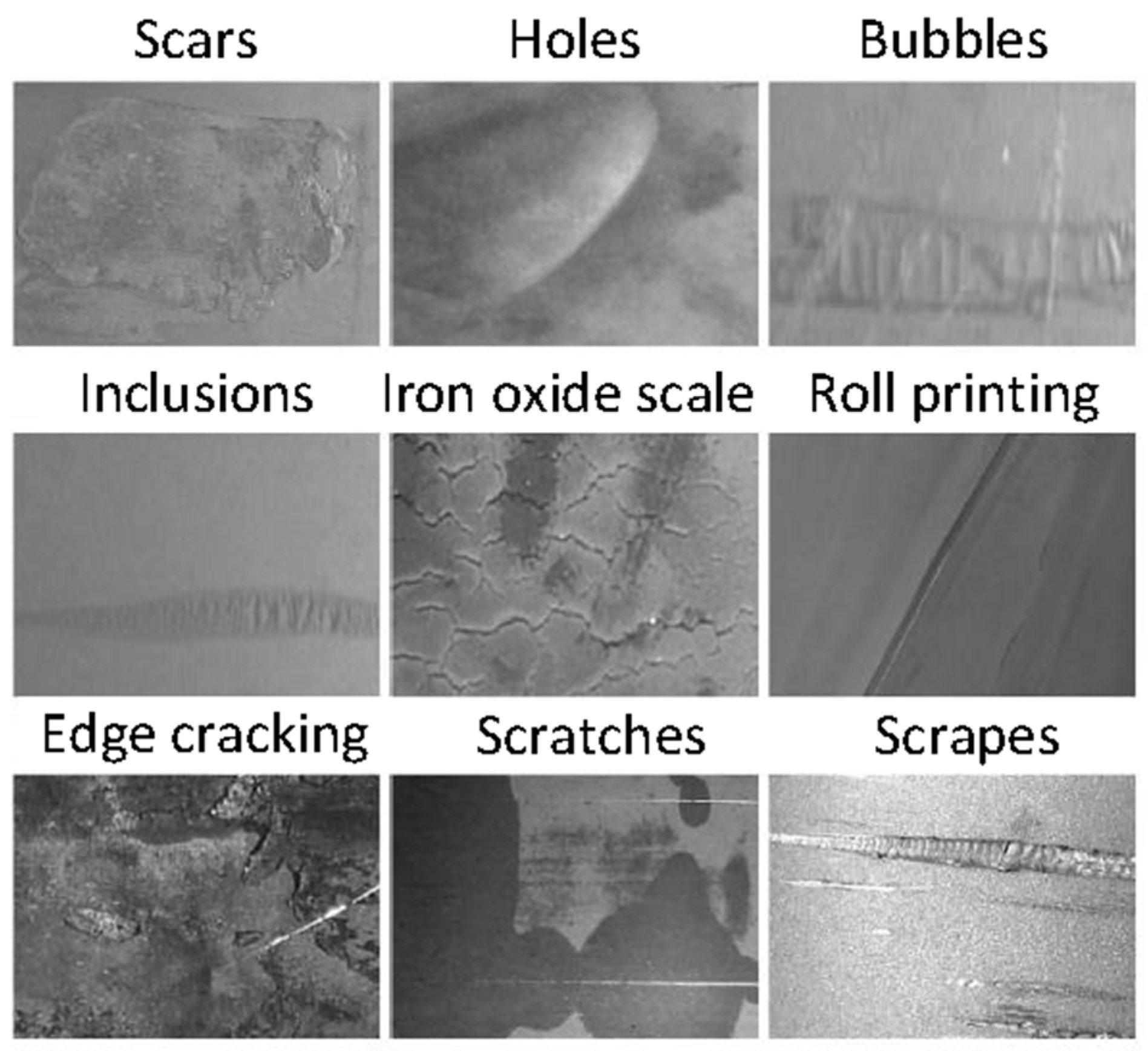
Hot-rolled steel plates will have some surface defects due to the production process and the steel billets; such defects are divided into steel defects and process defects according to the causes [35]. The structure of surface defects is shown in Figure 1. Scars are metal flakes with irregular shapes that attach to the surface of the steel strip. This defect can cause problems such as metal peeling or holes during subsequent processing and utilization. Gas pores are irregularly distributed round or elliptical convex hull defects on the surface of the steel strip, which can cause problems such as delamination or low welding during subsequent processing and utilization [36]. Inclusions are lumpy or elongated inclusive defects in the slab exposed on the surface of the steel strip after the inclusions or slag inclusions are rolled. Such defects will cause holes, cracks and delamination during subsequent processing. Iron oxide scale is a kind of surface defect formed by pressing an iron oxide scale into the surface of the steel strip during the hot rolling process. This defect will affect the surface quality and coating effect of the steel strip. Roll marks are irregularly distributed convex and concave defects on the surface of the steel strip, which can cause folding defects in the rolling process. Edge cracking is a phenomenon in which one or both sides of the steel strip edges are cracked along the length direction, which may cause problems such as interruption of the strip during the subsequent processing and utilization [37]. Scratches are a form of linear mechanical damage on the surface of the steel strip lower than the rolled surface. The scratched iron sheet is difficult to eliminate by pickling after oxidation, which can easily cause breakage or cracking. Scrapes are a form of mechanical damage on the surface of the steel strip in the form of points, strips or blocks. The iron oxide scale at the scrapes is challenging to remove by pickling. Problems such as bending and cracking may be caused [38].
3.2. Detection Technologies for Steel Plate’s Surface Defects
3.2.1. Traditional Detection Technology
Traditionally, technologies of detecting steel surface defects are divided into manual detection methods and non-destructive detection methods. Manual inspection is based on visual inspection and manual experience, which requires on-site observations in harsh environments, causing considerable damage to the health of the staff member; besides, solely relying on workers’ experience often causes problems, such as missed inspections, making it difficult to guarantee the quality of the steel plates [39]. Traditional non-destructive detection is divided into eddy current detection, infrared detection and magnetic leakage detection. Eddy current detection is suitable for detecting defects on the surface and lower layer of the steel plate, which requires a more extensive current guarantee. Hence, it consumes a lot of energy, and the surface of the steel plate must be at a constant temperature, making it unsuitable for industry requirements [40]. Infrared detection adds induction coils to the production process of industrial steel plates. If the steel billets pass by, the induced current will be generated on the surface; if a defect is found, the current will increase, which is an excellent way to detect defects. However, infrared detection can only be utilized in products with lower detection standards, and fewer types of defects can be detected [41]. Magnetic leakage detection is based on a proportional relationship between the volume of steel defects and the magnetic flux density. After calculating the density of magnetic leakage, the defect location and area of the steel can be calculated; however, this detection method is disadvantageous for surface detection [42]. As science and technology advances, a machine vision detection technology is proposed, which uses lasers and charge-coupled components to effectively detect the surface of steel plates after digitization.
3.2.2. Deep Learning Detection Technology
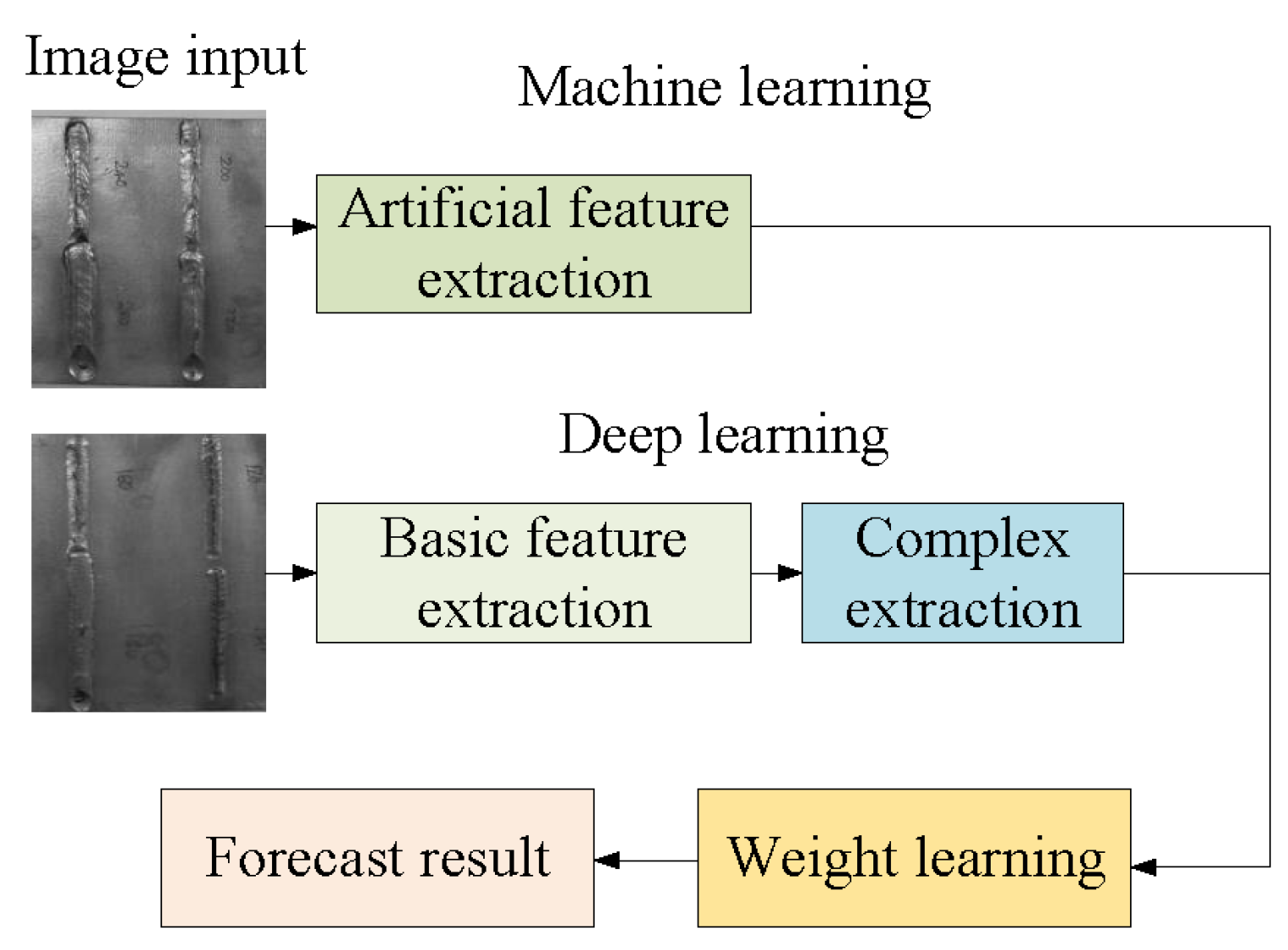
As deep learning technology advances continuously, it gradually presents apparent advantages in image recognition and classification. CNNs can extract image features. The detection ability of neural networks is improved by continuously increasing the number of layers and network widths of CNNs [43]. Such an improvement can effectively avoid subjectivity and inefficiency in the manual extraction process. Research on recognizing weld defect images is varied; especially, deep learning technology processes and organizes a single feature to quantify the abstract features according to the extraction principle, thereby using these features to classify and recognize images [44]. Figure 2 shows the difference between traditional machine learning and deep learning processes. Deep learning can obtain high-dimensional image features from the input data, fit the features and finally utilize the learning method of weights to increase the accuracy of classification prediction. However, while analyzing welds of industrial steel plates, deep learning cannot learn due to the lack of complete datasets; in addition, current research primarily focuses on improving the weld recognition ability; however, a complete automatic detection system has never been built, increasing the difficulty in actual industrial applications [45].
3.3. Image Preprocessing
3.3.1. Image Denoising
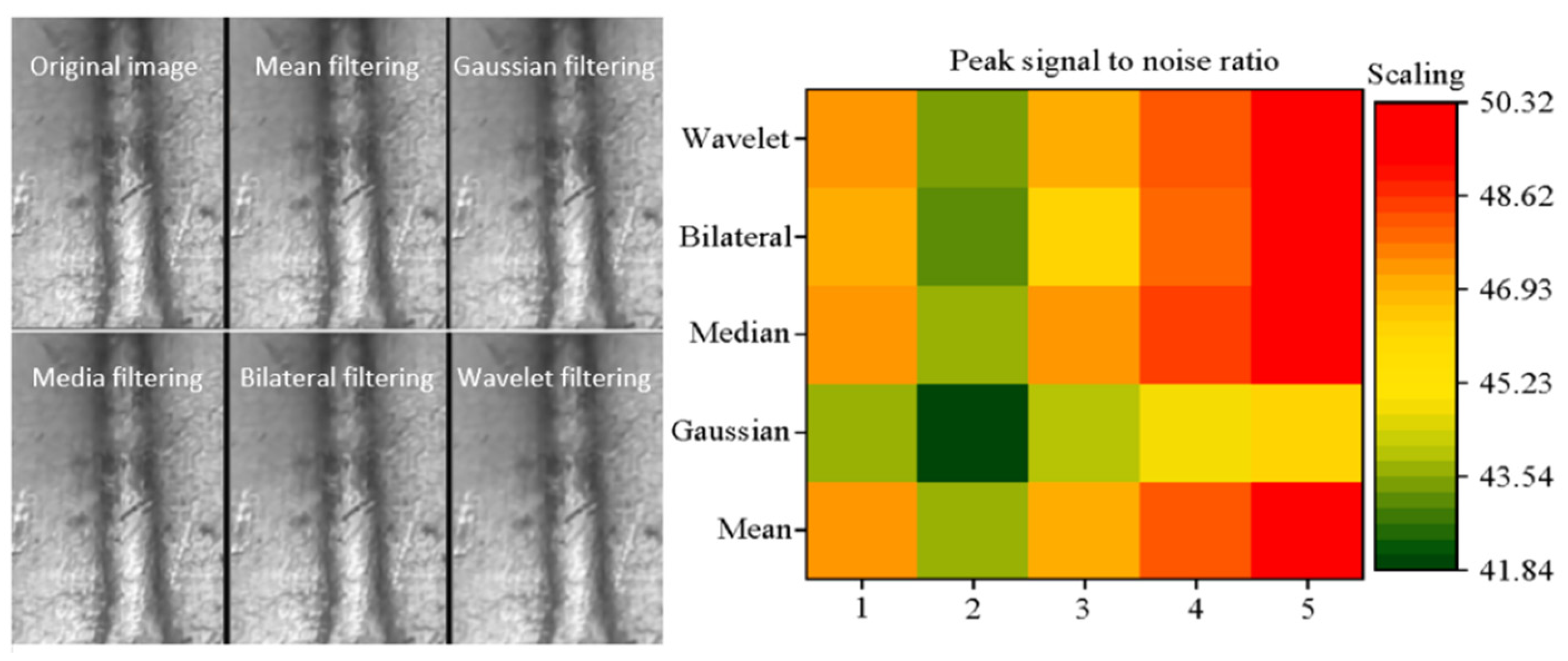
Image processing is the basis for effective weld detection. Here, image preprocessing aims to ensure that the image quality meets the requirements of deep learning. The weld images, provided by some enterprises, are observed, revealing a problem that, currently, some images often appear as dispersive white or black noise particles during digitization; meanwhile, during the radiography process, the exposure intensity will also cause problems, such as image contrast and grayscale degradation [46]. Therefore, image denoising is necessary. The typical image denoising methods include mean filtering, median filtering, Gaussian filtering, bilateral filtering and wavelet filtering, among which median filtering can effectively interfere with uniform pulses, enabling it to effectually maintain edge information after processing. However, such processing will cause the gray level to decrease. Gaussian filtering can process the details very well, but the images must conform to the Gaussian function distribution. Bilateral filtering can retain the edge information; nevertheless, the processing of other noises is inexplicit. Wavelet filtering has a good time-domain performance but a common processing effect on the frequency band [47]. Randomly, an image during processing is chosen and processed by the above five denoising methods to find the optimal processing method. Peak Signal-to-Noise Ratio (PSNR) and Mean Squared Error (MSE) are employed for evaluation. Specifically, the equations are as follows:
In Equations (1) and (2), 255 represents the maximum value of the image point color. is the gray pixel value of the image after denoising, is the gray pixel value of the input image and MN is the image pixel.
3.3.2. Image Enhancement
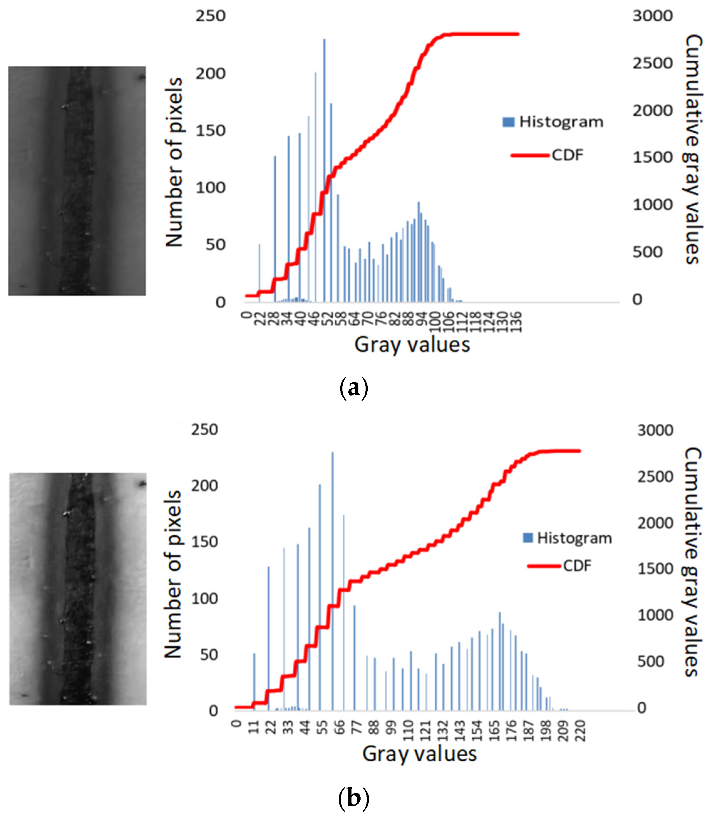
In welds, unreasonably adjusting the window width will cause image contrast reduction. Especially, edges of the defects are usually difficult to recognize, affecting the subsequent processing of the images. Therefore, image enhancement technology is employed to improve the contrast effectually [48]. First, images undergo grayscale processing; a specific histogram is obtained after statistical analysis. Then, the processed image is stretched according to its size to make its average gray value the segmentation standard so that the average grayscale will increase after processing. Finally, a dual-peak gray distribution image is obtained. The Sin function is used for nonlinear transformation and image stretching, which is shown in Equation (3):
In Equation (3), is the gray value after transformation, is the gray value before the transformation, a is the lowest gray value before the transformation and b is the highest gray value before the transformation. The value 127 represents the median value of the difference between the highest pixel value and the lowest pixel value, which is calculated as a fixed constant.
The whole image preprocessing process is based on C++/Python and OpenCV on the Visual Studio2013 platform.
3.4. Deep Learning Neural Networks
3.4.1. Convolution Neural Networks
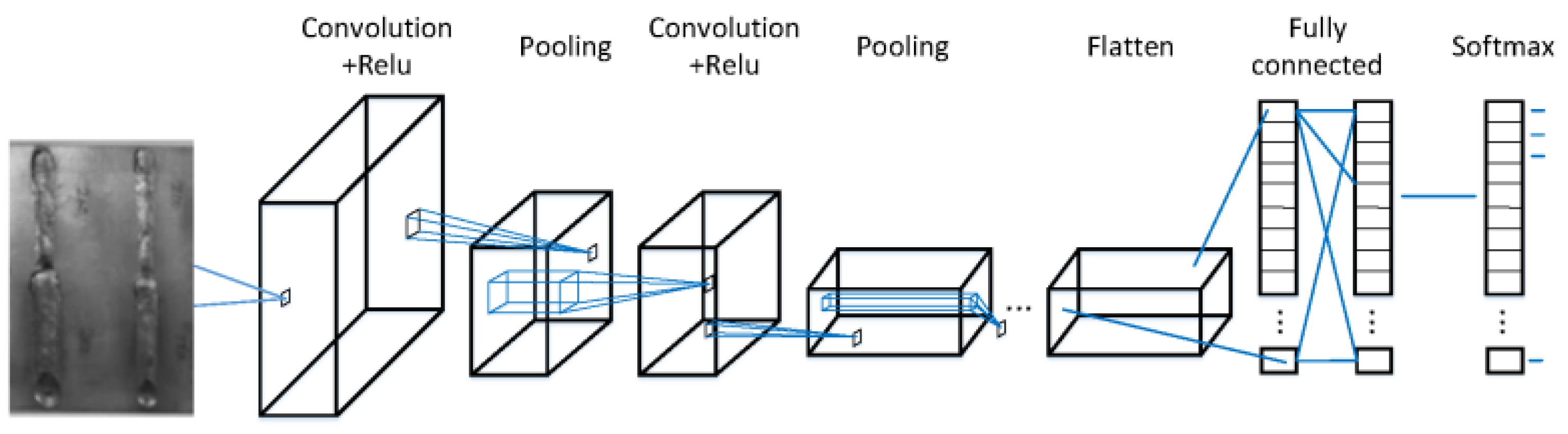
The CNN is a useful supervised deep learning model. It is a feed-forward neural network whose artificial neurons can respond to some surrounding units within the coverage [49]. CNNs are widely applied to image recognition, including AlexNet, Visual Geometry Group Nets (VGGNets) and other models that reduce the recognition error rate of CNNs on a typical ImageNet dataset. Generally, deep learning models have at least three hidden layers. As the number of hidden layers increases, the model’s parameters will also increase, thereby increasing the complexity of the model, providing the possibility to complete more complicated tasks. If a shallow model in which each layer of the network is fully connected is adopted for image classification and recognition, this model will contain many parameters. In the case of multiple hidden layers, the parameters contained in the model will exhibit explosive growth, causing adverse impacts on the space occupation, iterative calculation and convergence speed of the model. The hidden layers in CNNs can significantly reduce the number of parameters in the model via weight sharing and sparse connections, thereby increasing the training speed of the model [50]. Figure 3 shows the structure of the CNN.
In a CNN, the cross-entropy loss function for the classification error of the i-th sample is defined as:
The output of a single sample after passing the network is , and the corresponding sample loss value is:
The backpropagation rule of the CNN updates the weight of each neuron, making the overall error function of the model continuously decrease. The convolution process is defined as follows:
In Equation (6), is the number of convolutional layers in the model, is the number of convolution kernels, is the additive bias, is the activation function and is the input image. The convolutional collection layer is defined as:
In Equation (7), represents the data collection function, and represent the product bias and additive bias, respectively, and is the activation function.
3.4.2. Transfer Learning
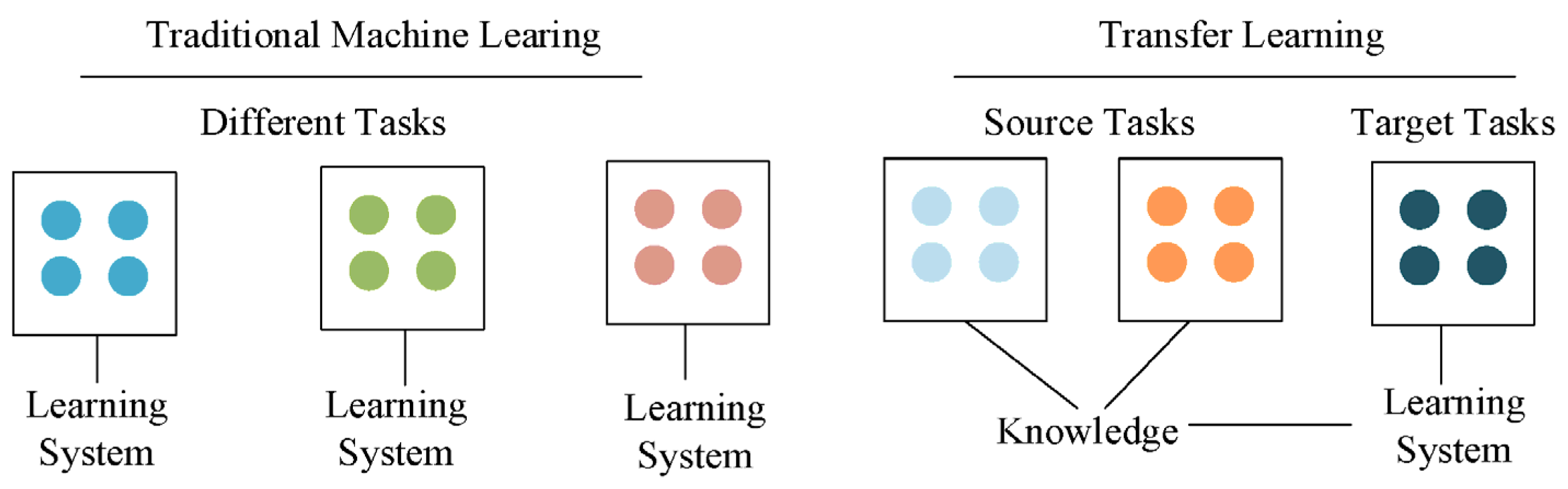
TL can meet the end-to-end needs in practical applications with more expressive features. It is a deep learning method that uses existing knowledge to solve problems in different but related domains. TL has become another popular research direction in deep learning [51]. Compared with traditional machine learning methods, TL directly improves the learning effect on different tasks, focuses on applying good source domain task knowledge to different but related target problems, and enables computers to learn by analogy without relying on big data for initial learning in every field. The training of traditional machine learning models requires labeled data from various fields, while data in different fields do not have TL performance on the same model. TL can utilize existing knowledge to learn new knowledge. Figure 4 shows the structural comparison between traditional machine learning and transfer learning. TL can organically utilize the knowledge in the source domain to better model the target domain under the condition of changes in data distribution, feature dimensions and model output conditions [52].
3.5. Deep Learning-Based Image Defect Recognition Model
Based on the above questions, the model is divided into four processes. The first process is establishing a crack defect dataset. The second process is building a deep learning process based on the above dataset. The third process is using the improved CNN for data learning and feature extraction. Finally, TL trains and classifies the corresponding images based on the original VGG16 model.
(1) Deep learning process: The number of convolutional layers is 3, the size of the convolution kernel is 5 × 5 and the depth is 6, 12 and 16, respectively. The initial weight of each convolution kernel is a truncated customarily distributed random number with a mean value of 0 and a standard deviation of 0.1. Each convolutional layer is composed of several convolutional units, and the backpropagation algorithm optimizes the parameters of the convolutional unit. More complex features are extracted iteratively by extracting different features of the input. N represents normalization, which can constrain the convolution result. E denotes the ELU activation function, which can de-linearize the calculation result. P signifies the pooling layer, the size of its convolution kernel is set to 2 × 2 and the moving step size is 2. Both the convolutional layer and the pooling layer are filled with all zeros. FC refers to the fully connected layer, and the number of nodes is reduced to 60 through two fully connected layers. The designed CNN comprises five types of defects to be classified and recognized. Hence, the number of output layer S is set to 5.
(2) CNN improvement: ReLU’s unilateral inhibition capability can make the neurons in the network sparsely activate, thereby better mining relevant features, fitting training data and solving the gradient exploding/vanishing problem. In the present work, an improved ELU nonlinear activation function is adopted. ELU can integrate the advantages of the Sigmoid and ReLU functions. While maintaining the unsaturation on the right side of the function, it increases the soft saturation on the left side of the function so that the unsaturated part can alleviate the gradient vanishing during model training. Moreover, soft saturation can make the model more robust to input changes or noises. The pooling process is one of the critical steps in the CNN; however, the classic pooling model has some shortcomings in pooling domain feature extraction. Excessive noises during image feature extraction caused by the pooling approach can result in difficulty in optimal feature selection. In addition, the lack of selective importance extraction of each feature will also affect the final recognition effect. Hence, improvements can be made based on classic pooling approaches. In the present work, an adaptive pooling approach that comprehensively considers the pooling domain and feature distribution is adopted so that the pooling model can select the optimal features under different feature distributions.
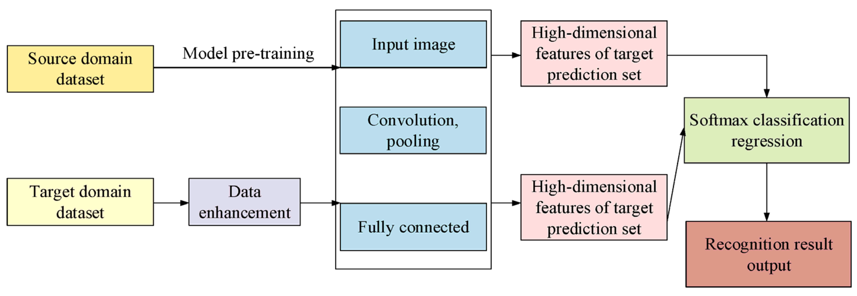
(3) TL process: The first step is model pre-training, performed on a large, challenging image dataset. This dataset contains sufficient image data resources so that the VGG16 model can obtain the weights of each layer by training the source domain dataset. The second step is model transfer. Based on model pre-training, its convolutional layer and pooling layer parameters are retained as the frozen layer. The fully connected layer and the input image size of the model are changed to adapt to the model input requirements and defect recognition types. Afterward, the data are retrained, and finally, tasks of classification and recognition are completed. The third step is model fine-tuning. This operation can perform good fitting and extract image features during the training process, initialize the model during the target domain training and utilize the backpropagation algorithm and Stochastic Gradient Descent (SGD) algorithm to fine-tune and correct the model parameters until the training task is completed or the training end condition is reached. Eventually, a model with excellent generalization ability is obtained. Here, the SoftMax classifier is adopted to classify and output the recognition results. The specific structure is presented in Figure 5.
3.6. Experimental Data and Performance Evaluation
3.6.1. Experimental Environment and Data
This experiment is based on the Linux Ubuntu 16.04 operating system, Inter (R) Core (TM) I5-2400 Central Processing Unit (CPU) @3.10 GHz, using python language to implement under the TensorFlow framework and Spyder platform of Anaconda. The number of iterations is set to 250 according to the model accuracy and training time. The SGD algorithm is adopted. The momentum parameter is 0.9, the Batch_Size is 20 and the learning rate is 1 × 10⁻⁴. Table 1 shows the corresponding environment for the experiment.
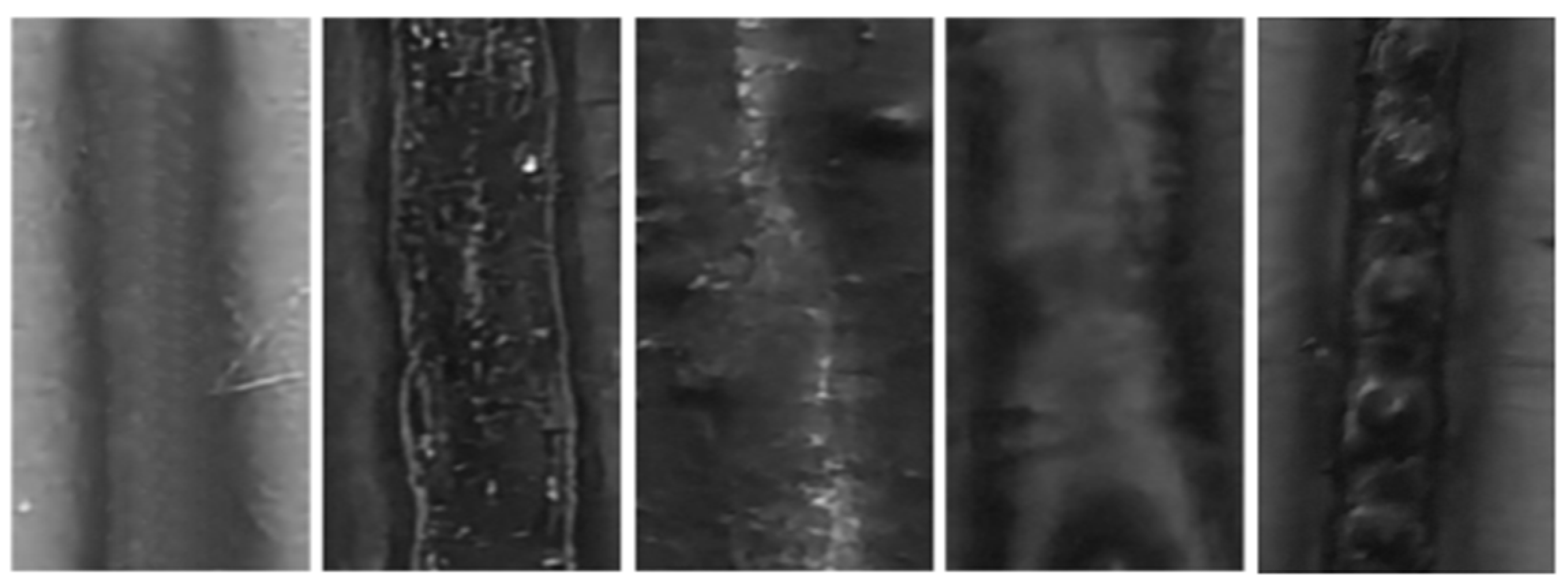
The VGG16 model is employed for TL. The pre-trained model comes from the ImageNet dataset, the world’s largest database for image recognition, containing 15 million images and covering the images of all objects in life [53]. The image data in this work come from the steel plate production line of an actual factory. The laser welding of carbon steel plates and stainless steel plates is studied and the appearance of these two types of steel plates is inconsistent under the definition of the same defect type. Affected by the change in welding environment, various welding defects will be produced in laser welding. A total of 1030 original steel plate weld images were collected by an industrial camera, visual light source and laser welding machine tool. Each original weld image is 5 million pixels and each original weld image contains various defects. We mixed all these asymmetric image data. Five different types of weld images can be obtained by cutting the original image. Figure 6 illustrates the detailed information of some images. From left to right were flawless, cracks, lack of fusion, lack of penetration and gas pores.
3.6.2. Image Partition and Labeling
A total of 5200 usable weld defect images were obtained through image data enhancement, containing five types: gas pores, cracks, lack of fusion, lack of penetration and flawless. These image data were stored in five folders according to the defect types, and the file labels were set from 1 to 5, in turn. All data were divided into a training set, a validation set and a test set by 8:1:1. The labels corresponding to the number of images in each image dataset are summarized in Table 2. The image processing time was 20 s.
3.6.3. Model Performance Evaluation
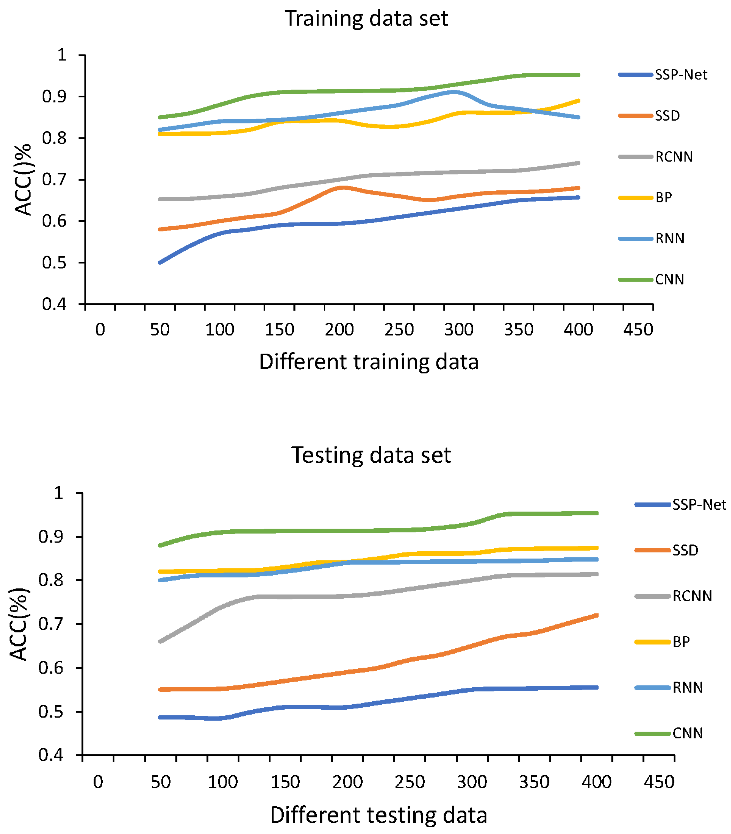
Accuracy (ACC) is the comparison indicator of model performance evaluation, representing the proportion of processed samples correctly classified as positive samples [54]. The calculation of ACC is Equation (8), where is the number of correctly predicted defect images and is the number of actual defect images. The algorithms selected include Spatial Pyramid Pooling Networks (SPP-Net), Single Shot MultiBox Detector (SSD), Region-CNN (RCNN), CNN, BPNN, and Recursive Neural Networks (RNN), totaling six algorithms for comparative analysis.
4. Results and Discussion
4.1. Image Processing Results of Weld Defects
Figure 7 shows the image effects and the quantization results processed by the filtering methods. Median filtering can present a clear edge area of the steel plate defect, while other denoising algorithms cannot. Furthermore, in all the images, especially in the fifth image, the highest PSNR reaches 50.31 dB, indicating that the effect of median filtering is better than other methods.
Figure 8 demonstrates the weld image and grayscale histogram before and after the Sin function transformation. The gray value of the image after the Sin function transformation increases significantly, and the contrast image is enhanced considerably, showing the effectiveness of the image enhancement technology applied.
4.2. Performance Comparison of Different Training Models
Figure 9 presents the comparison results of different training models’ performances. As the amount of data increases, the defect detection performance of the model continuously improves, and the training set and the test set show the same trend, indicating the correctness of this training process. The proposed CNN model presents the best performance among different algorithm models, whose average ACC is above 92%, followed by the RNN model because of its multiple input processes that can reduce the model loads. The above results show that the weld defect detection and recognition model based on deep learning technology has excellent performance.
4.3. Comparative Experiment of Industrial Weld Defect Images
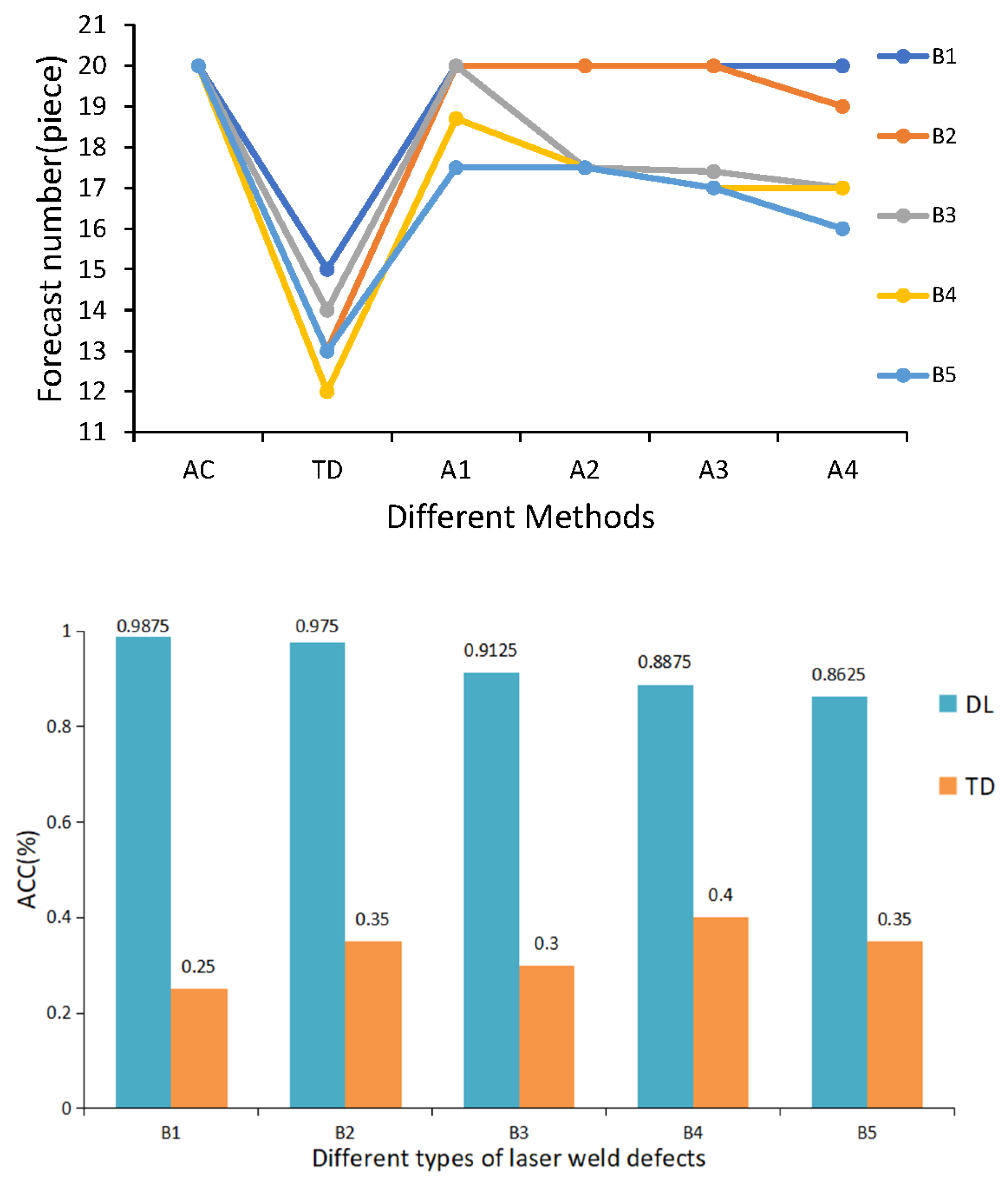
Figure 10 shows the experimental results of comparisons among industrial weld defect images. As the number of convolutional layers increases, the performance of the model decreases. The proposed model presents a higher ACC than traditional machine learning algorithms under different defect types, showing excellent robustness. The performance of the proposed weld detection algorithm is significantly improved. The highest defect detection ACC reaches 98.75%, which effectively improves the automation degree of industrial weld detection and recognition.
4.4. Results of Other Performance Indicators
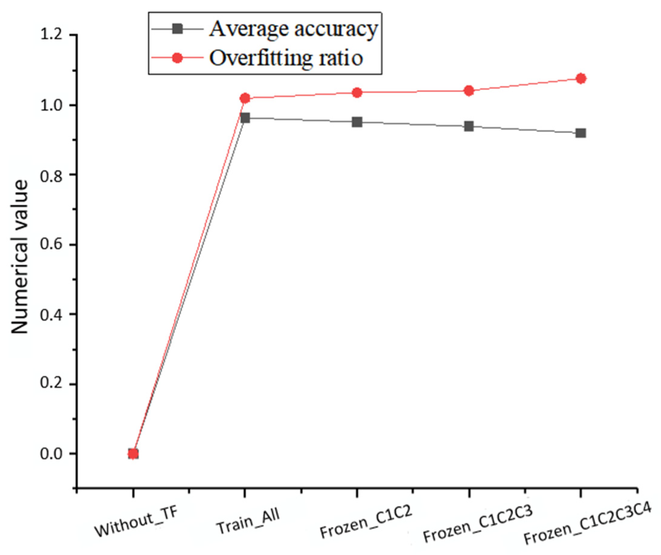
Figure 11 shows the result curves of the model accuracy and over-fitting rate under different experimental methods.
The average accuracy and over-fitting ratio of 250 iterations of the model in various experimental methods are shown in Figure 11; without_TF directly uses the first VGG16 model without training ImageNet datasets or learning how to migrate. Train_All means to create the VGG16 model and improve all training and network parameters of different layers without freezing the model through sufficient data training and migration training. Frozen_Cx represents an experimental method that freezes the fine-tuning model of X-layer training parameters of the heterogeneous migration model. The analysis in Figure 11 is a migration recognition task of the image dataset for the weld defect detection. The without_TF method lacks enough data to train the model, the extraction ability and feature representation are relatively low, the recognition efficiency is low, there is a serious over-fitting problem, the performance is poor, and it has not been calculated.
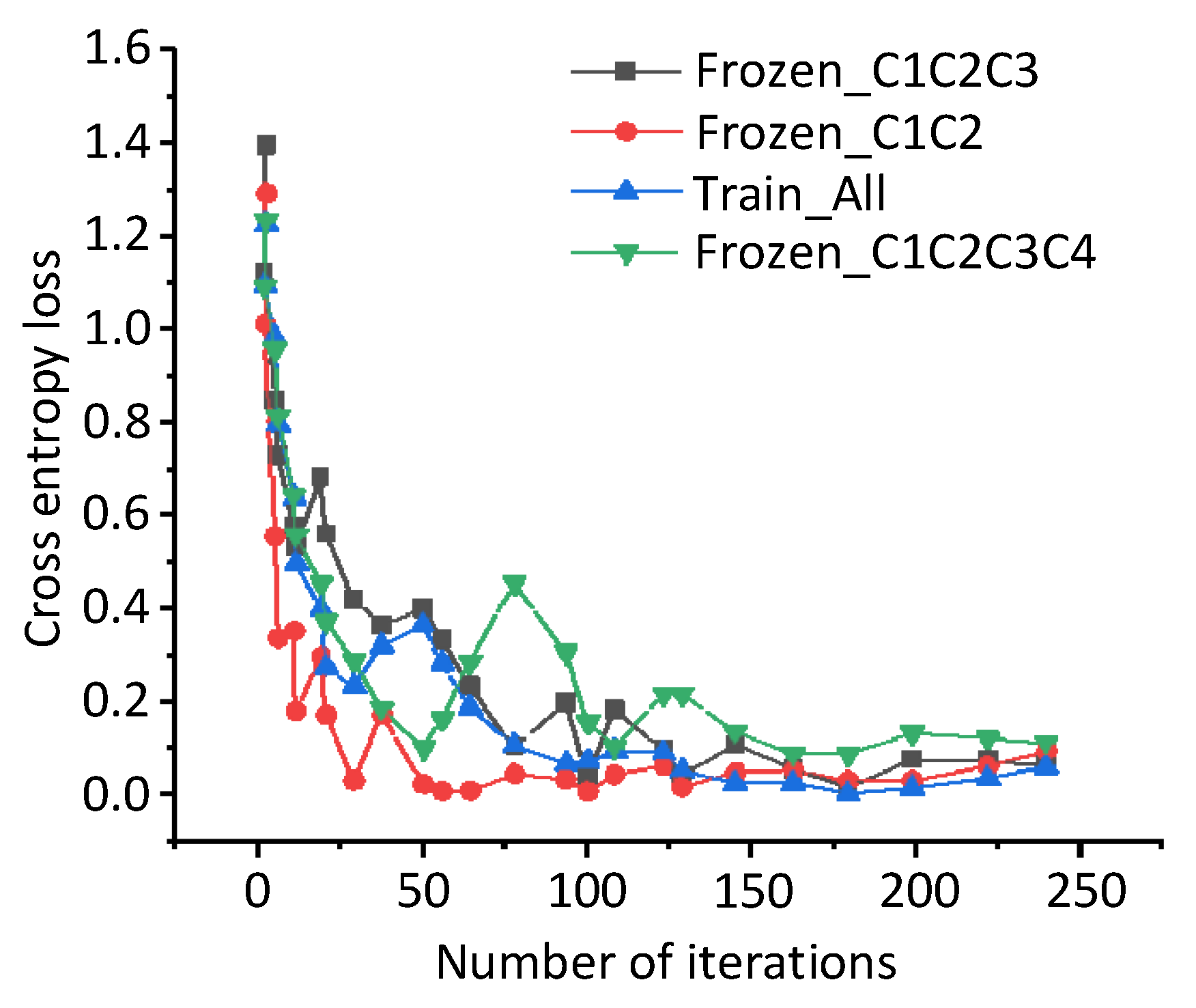
Figure 12 shows the results of cross-entropy loss under different iteration times. When the source domain model features and training parameters are fully mounted to fine-tune the entire model, the learning ability of the target domain will be rapidly improved. Since the adjustment process from the beginning to the end gradually refines the underlying features of the original input, the feature expression ability between layers is more vital. In that case, the abstract features of the image can be better integrated, presenting better results. The more frozen convolutional layers there are, the lower the accuracy of the model, and the higher the over-fitting ratio of the model.
The results in Table 3 can be analyzed from two aspects: experimental methods and types of defects. First, the test results are consistent with the results obtained from the training and verification data regarding different experimental methods. When the source domain model features and training parameters are fully mounted to fine-tune the entire model, the model can provide better generalization ability, and the recognition result is also the best. With the continuous increase in the number of frozen layers, the test accuracy of the model has decreased, and the test accuracy of the weld inspection image has also gradually decreased. Second, regarding different types of defects, the image test accuracy of GP and FL is higher than that of other defects. The test accuracy of CK is the lowest due to the small data amount. The test results for LOF and LOP images are not ideal because their shape, size, color and other features are similar. During the training process, the image features are prone to confusion, so errors are prone to occur during testing. Using TL for small sample weld defect images can provide a better recognition effect regarding the computing power and sample data volume.
5. Conclusions
A deep learning-based weld defect detection and image defect recognition model is proposed regarding the GP, FL, LOF, LOP and CK defects in industrial welding, and the recognition accuracy of the model reaches 98.75%. The size of the whole model is 232 M, and the test time of a single image input into the model is about 200 ms. The model uses image denoising processing and enhancement to segment the target image. Cross datasets are used regarding the insufficient training data in deep neural networks. This model improves activation function and adaptive pooling. Regarding the recognition problems of DNN on the weld defect image dataset, TL is employed to shorten the model training time through simple adjustment and hyperparameter adjustment. This model can overcome the shortcomings of traditional approaches. It provides strong robustness and high recognition accuracy in the task of identifying weld defect images. Nevertheless, several shortcomings are found. First, since there are no high-precision industrial sample datasets, if the images of industrial weld defect samples can be utilized to build a high-quality database, the model accuracy can be improved effectively. Second, given the increasing number of industrial datasets, building more complex neural network models is necessary. This requires using the Graphic Processing Unit (GPU) distributed optimization algorithms to improve the efficiency of algorithm operation. Finally, although the content of TL is introduced, it is an addition to CNNs. Therefore, the problem of sample appearance caused by TL needs to be solved. In the future, these aspects will be researched and analyzed more deeply, in an effort to help steel enterprises master the automated detection technology of weld defects, get rid of technology monopoly and truly realize high-quality development.
Author Contributions
Investigation, J.X.; Resources, Y.F.; Software, Y.C.; Validation, J.X.; Writing—original draft, H.D.; Writing—review & editing, Y.C. All authors have read and agreed to the published version of the manuscript.
Funding
This research received no external funding.
Institutional Review Board Statement
Not applicable.
Informed Consent Statement
Not applicable.
Data Availability Statement
Not applicable.
Conflicts of Interest
The authors declare no conflict of interest.
References
- Qiao, J.; Yu, P.; Wu, Y.; Chen, T.; Du, Y.; Yang, J. A Compact Review of Laser Welding Technologies for Amorphous Alloys. Metals 2020, 12, 1690. [Google Scholar] [CrossRef]
- Zapata, J.; Vilar, R.; Ruiz, R. An adaptive-network-based fuzzy inference system for classification of welding defects. NDT E Int. 2010, 43, 191–199. [Google Scholar] [CrossRef]
- Gruse, J.N.; Streeter, M.J.V.; Thornton, C.; Armstrong, C.D.; Baird, C.D.; Bourgeois, N.; Cipiccia, S.; Finlay, O.J.; Gregory, C.D.; Katzir, Y.; et al. Application of compact laser-driven accelerator X-ray sources for industrial imaging. Nucl. Instrum. Methods Phys. Res. Sect. A Accel. Spectrom. Detect. Assoc. Equip. 2020, 983, 164369. [Google Scholar]
- Drotár, A.; Zubko, P.; Mašlejová, A.; Kalmár, P.; Vranec, P.; Hockicková, S.; Demčáková, M.; Hrabčáková, L. Defects of Steel Sheets Joined by Laser Welding. Defect Diffus. Forum 2020, 405, 240–244. [Google Scholar] [CrossRef]
- Schmid, M.; Bhogaraju, S.K.; Liu, E.; Elger, G. Comparison of Nondestructive Testing Methods for Solder, Sinter, and Adhesive Interconnects in Power and Opto-Electronics. Appl. Sci. 2020, 10, 8516. [Google Scholar] [CrossRef]
- Ricketts, J. Film-Screen Radiography in Bachelor’s Degree Program Curriculum. Radiol. Technol. 2016, 88, 234–236. [Google Scholar]
- Vorobeychikov, S.E.; Chakhlov, S.V.; Udod, V.A. A Cumulative sums algorithm for segmentation of digital X-ray images. J. Nondestruct. Eval. 2019, 38, 78–86. [Google Scholar] [CrossRef]
- Roshani, M.; Phan, G.T.; Ali, P.J.M.; Roshani, G.H.; Hanus, R.; Duong, T.; Corniani, E.; Nazemi, E.; Kalmoun, E.M. Evaluation of flow pattern recognition and void fraction measurement in two phase flow independent of oil pipeline’s scale layer thickness. Alex. Eng. J. 2021, 60, 1955–1966. [Google Scholar] [CrossRef]
- Nisar, M.U.; Voghoei, S.; Ramaswamy, L. Caching for pattern matching queries in time evolving graphs: Challenges and approaches. In Proceedings of the 2017 IEEE 37th International Conference on Distributed Computing Systems (ICDCS), Atlanta, GA, USA, 5–8 June 2017; pp. 2352–2357. [Google Scholar]
- Tasoujian, S.; Salavati, S.; Franchek, M.A.; Grigoriadis, K.M. Robust delay-dependent LPV synthesis for blood pressure control with real-time Bayesian parameter estimation. IET Control. Theory Appl. 2020, 14, 1334–1345. [Google Scholar] [CrossRef]
- Karimi, M.; Jahanshahi, A.; Mazloumi, A.; Sabzi, H.Z. Border gateway protocol anomaly detection using neural network. In Proceedings of the 2019 IEEE International Conference on Big Data (Big Data), Los Angeles, CA, USA, 9–12 December 2019; pp. 6092–6094. [Google Scholar]
- Moaveni, B.; Fathabadi, F.R.; Molavi, A. Supervisory predictive control for wheel slip prevention and tracking of desired speed profile in electric trains. ISA Trans. 2020, 101, 102–115. [Google Scholar] [CrossRef] [PubMed]
- Voghoei, S.; Tonekaboni, N.H.; Yazdansepas, D.; Soleymani, S.; Farahani, A.; Arabnia, H.R. Personalized Feedback Emails: A Case Study on Online Introductory Computer Science Courses. In Proceedings of the 2020 ACM Southeast Conference, Tampa, FL, USA, 2–4 April 2020; pp. 18–25. [Google Scholar]
- Shih, P.C.; Hsu, C.C.; Tien, F.C. Automatic Reclaimed Wafer Classification Using Deep Learning Neural Networks. Symmetry 2020, 12, 705. [Google Scholar] [CrossRef]
- Brachmann, A.; Redies, C. Using Convolutional Neural Network Filters to Measure Left-Right Mirror Symmetry in Images. Symmetry 2016, 8, 144. [Google Scholar] [CrossRef] [Green Version]
- Zhang, M.; Diao, M.; Gao, L.; Liu, L. Neural Networks for Radar Waveform Recognition. Symmetry 2017, 9, 75. [Google Scholar] [CrossRef] [Green Version]
- Hou, W.; Wei, Y.; Jin, Y.; Zhu, C. Deep features based on a DCNN model for classifying imbalanced weld flaw types. Measurement 2019, 131, 482–489. [Google Scholar] [CrossRef]
- Shevchik, S.; Le-Quang, T.; Meylan, B.; Farahani, F.V.; Olbinado, M.P.; Rack, A.; Masinelli, G.; Leinenbach, C.; Wasmer, K. Supervised deep learning for real-time quality monitoring of laser welding with X-ray radiographic guidance. Sci. Rep. 2020, 10, 3389. [Google Scholar] [CrossRef] [Green Version]
- Ajmi, C.; Zapata, J.; Martínez-Álvarez, J.J.; Doménech, G.; Ruiz, R. Using Deep Learning for Defect Classification on a Small Weld X-ray Image Dataset. J. Nondestruct. Eval. 2020, 39, 68. [Google Scholar] [CrossRef]
- Ajmi, C.; Zapata, J.; Elferchichi, S.; Zaafouri, A.; Laabidi, K. Deep Learning Technology for Weld Defects Classification Based on Transfer Learning and Activation Features. Adv. Mater. Sci. Eng. 2020, 2020, 1574350. [Google Scholar] [CrossRef]
- Boikov, A.; Payor, V.; Savelev, R.; Kolesnikov, A. Synthetic Data Generation for Steel Defect Detection and Classification Using Deep Learning. Symmetry 2021, 13, 1176. [Google Scholar] [CrossRef]
- Javadi, Y.; Sweeney, N.E.; Mohseni, E.; MacLeod, C.N.; Lines, D.; Vasilev, M.; Qiu, Z.; Vithanage, R.K.; Mineo, C.; Stratoudaki, T. In-process calibration of a non-destructive testing system used for in-process inspection of multi-pass welding. Mater. Des. 2020, 195, 108981. [Google Scholar] [CrossRef]
- Boaretto, N.; Centeno, T.M. Automated detection of welding defects in pipelines from radiographic images DWDI. NDT E Int. 2017, 86, 7–13. [Google Scholar] [CrossRef]
- Bestard, G.A.; Sampaio, R.C.; Vargas, J.A.; Alfaro, S.C.A. Sensor fusion to estimate the depth and width of the weld bead in real time in GMAW processes. Sensors 2018, 18, 962. [Google Scholar] [CrossRef] [Green Version]
- Vasilev, M.; MacLeod, C.; Galbraith, W.; Pierce, G.; Gachagan, A. In-process ultrasonic inspection of thin mild steel plate GMAW butt welds using non-contact guided waves. In Proceedings of the 46th Annual Review of Progress in Quantitative Nondestructive Evaluation QNDE2019, Portland, OR, USA, 14–19 July 2019; pp. 115–124. [Google Scholar]
- Gao, Y.; Gao, L.; Li, X.; Yan, X. A semi-supervised convolutional neural network-based method for steel surface defect recognition. Robot. Comput.-Integr. Manuf. 2020, 61, 101825. [Google Scholar] [CrossRef]
- Li, C.; Wang, Q.; Jiao, W.; Johnson, M.; Zhang, Y. Deep Learning-Based Detection of Penetration from Weld Pool Reflection Images. Weld. J. 2020, 99, 239s–345s. [Google Scholar] [CrossRef]
- Sony, S.; Dunphy, K.; Sadhu, A.; Capretz, M. A systematic review of convolutional neural network-based structural condition assessment techniques. Eng. Struct. 2021, 226, 111347. [Google Scholar] [CrossRef]
- Chen, F.-C.; Jahanshahi, M.R. NB-CNN: Deep learning-based crack detection using convolutional neural network and Naïve Bayes data fusion. IEEE Trans. Ind. Electron. 2017, 65, 4392–4400. [Google Scholar] [CrossRef]
- Davis, D.S. Object-based image analysis: A review of developments and future directions of automated feature detection in landscape archaeology. Archaeol. Prospect. 2019, 26, 155–163. [Google Scholar] [CrossRef]
- Li, L.; Xiao, L.; Liao, H.; Liu, S.; Ye, B. Welding quality monitoring of high frequency straight seam pipe based on image feature. J. Mater. Process. Technol. 2017, 246, 285–290. [Google Scholar] [CrossRef]
- Gao, X.; Du, L.; Xie, Y.; Chen, Z.; Zhang, Y.; You, D.; Gao, P.P. Identification of weld defects using magneto-optical imaging. Int. J. Adv. Manuf. Technol. 2019, 105, 1713–1722. [Google Scholar] [CrossRef]
- Bashar, A. Survey on evolving deep learning neural network architectures. J. Artif. Intell. 2019, 1, 73–82. [Google Scholar]
- Malarvel, M.; Singh, H. An autonomous technique for weld defects detection and classification using multi-class support vector machine in X-radiography image. Optik 2021, 231, 166342. [Google Scholar] [CrossRef]
- Chu, M.; Zhao, J.; Liu, X.; Gong, R. Multi-class classification for steel surface defects based on machine learning with quantile hyper-spheres. Chemom. Intell. Lab. Syst. 2017, 168, 15–27. [Google Scholar] [CrossRef]
- Zhou, S.; Chen, Y.; Zhang, D.; Xie, J.; Zhou, Y. Classification of surface defects on steel sheet using convolutional neural networks. Mater. Technol. 2017, 51, 123–131. [Google Scholar]
- Gong, R.; Wu, C.; Chu, M. Steel surface defect classification using multiple hyper-spheres support vector machine with additional information. Chemom. Intell. Lab. Syst. 2018, 172, 109–117. [Google Scholar] [CrossRef]
- Chu, M.; Liu, X.; Gong, R.; Liu, L. Multi-class classification method using twin support vector machines with multi-information for steel surface defects. Chemom. Intell. Lab. Syst. 2018, 176, 108–118. [Google Scholar] [CrossRef]
- Li, J.; Su, Z.; Geng, J.; Yin, Y. Real-time detection of steel strip surface defects based on improved yolo detection network. IFAC-PapersOnLine 2018, 51, 76–81. [Google Scholar] [CrossRef]
- AbdAlla, A.N.; Faraj, M.A.; Samsuri, F.; Rifai, D.; Ali, K.; Al-Douri, Y. Challenges in improving the performance of eddy current testing. Meas. Control. 2019, 52, 46–64. [Google Scholar] [CrossRef] [Green Version]
- Wu, P.; Chen, Z.; Jile, H.; Zhang, C.; Xu, D.; Lv, L. An infrared perfect absorber based on metal-dielectric-metal multi-layer films with nanocircle holes arrays. Results Phys. 2020, 16, 102952. [Google Scholar] [CrossRef]
- Wu, D.; Liu, Z.; Wang, X.; Su, L. Composite magnetic flux leakage detection method for pipelines using alternating magnetic field excitation. NDT E Int. 2017, 91, 148–155. [Google Scholar] [CrossRef]
- Yoo, Y.; Baek, J.-G. A novel image feature for the remaining useful lifetime prediction of bearings based on continuous wavelet transform and convolutional neural network. Appl. Sci. 2018, 8, 1102. [Google Scholar] [CrossRef] [Green Version]
- Dung, C.V.; Sekiya, H.; Hirano, S.; Okatani, T.; Miki, C. A vision-based method for crack detection in gusset plate welded joints of steel bridges using deep convolutional neural networks. Autom. Constr. 2019, 102, 217–229. [Google Scholar] [CrossRef]
- Shin, S.; Jin, C.; Yu, J.; Rhee, S. Real-time detection of weld defects for automated welding process base on deep neural network. Metals 2020, 10, 389. [Google Scholar] [CrossRef] [Green Version]
- Yang, M.; Ma, H.-h.; Shen, Z.-W.; Xu, J. Application of Colloid Water Covering on Explosive Welding of AA1060 Foil to Q235 Steel Plate. Propellants Explos. Pyrotech. 2020, 45, 453–462. [Google Scholar]
- Elhoseny, M.; Shankar, K. Optimal bilateral filter and convolutional neural network based denoising method of medical image measurements. Measurement 2019, 143, 125–135. [Google Scholar] [CrossRef]
- Xiao, B.; Tang, H.; Jiang, Y.; Li, W.; Wang, G. Brightness and contrast controllable image enhancement based on histogram specification. Neurocomputing 2018, 275, 2798–2809. [Google Scholar] [CrossRef]
- Yao, P.; Wu, H.; Gao, B.; Tang, J.; Zhang, Q.; Zhang, W.; Yang, J.J.; Qian, H. Fully hardware-implemented memristor convolutional neural network. Nature 2020, 577, 641–646. [Google Scholar] [CrossRef] [PubMed]
- Fu, Y.; Aldrich, C. Flotation froth image recognition with convolutional neural networks. Miner. Eng. 2019, 132, 183–190. [Google Scholar] [CrossRef]
- Choi, E.; Jo, H.; Kim, J. A Comparative Study of Transfer Learning–based Methods for Inspection of Mobile Camera Modules. IEIE Trans. Smart Process. Comput. 2018, 7, 70–74. [Google Scholar] [CrossRef]
- Ferguson, M.K.; Ronay, A.; Lee, Y.-T.T.; Law, K.H. Detection and segmentation of manufacturing defects with convolutional neural networks and transfer learning. Smart Sustain. Manuf. Syst. 2018, 2, 137–164. [Google Scholar] [CrossRef]
- Chrabaszcz, P.; Loshchilov, I.; Hutter, F. A Downsampled Variant of ImageNet as an Alternative to the CIFAR Datasets. arXiv 2017, arXiv:1707.08819. [Google Scholar]
- Luo, X.; Lam, K.P.; Chen, Y.; Hong, T. Performance evaluation of an agent-based occupancy simulation model. Build. Environ. 2017, 115, 42–53. [Google Scholar] [CrossRef] [Green Version]
Figure 1.
Surface defects of steel plate.

Figure 2.
Differences between traditional machine learning and deep learning.

Figure 3.
Structure of CNN.

Figure 4.
Structure comparison of traditional learning and TL.

Figure 5.
Deep learning-based image defect recognition model.

Figure 6.
Some collected weld images.

Figure 7.
Image effects and the quantization results processed by the filtering methods.

Figure 8.
Weld image and grayscale histogram (a) before and (b) after Sin function transformation.

Figure 9.
Performance comparison of different training models.

Figure 10.
Comparative experiment of industrial weld defect images. AC represents the original number of steel plates; TD represents the results of using traditional machine learning algorithms; A1–A4 represent the results using the VGG16 model for sufficient training, 12-layer training, 123-layer training and 1234-layer training, respectively; B1–B5 represent practical problems such as pores, cracks, lack of fusion, lack of penetration and flawless.

Figure 11.
Model accuracy and overfitting ratio results using different experimental methods.

Figure 12.
Cross entropy loss of different experimental methods.


Table 1.
Experimental environment.
| Software and Hardware | Specific Configuration Information |
|---|---|
| Central Processing Unit | Inter(R)-Core (TM) I5-2400 |
| RAM | DDR4 16 G |
| CPU Hertz | 3.10 GHz |
| Operating system | Ubuntu 16.04 |
| Programming environment | Python 3.5 |
Table 2.
Image data partition and labeling.
| Type of Defect | Gas Pores (GP) | Flawless (FL) | Lack of Fusion (LOF) | Lack of Penetration (LOP) | Cracks (CK) |
|---|---|---|---|---|---|
| Training set | 1200 | 1040 | 920 | 680 | 320 |
| Validation set | 150 | 130 | 115 | 85 | 40 |
| Test set | 150 | 130 | 115 | 85 | 40 |
| Label | 1 | 2 | 3 | 4 | 5 |
Table 3.
Test set classification results.
| Type of Defect | GP | FL | LOF | LOP | CK | ACC/% |
|---|---|---|---|---|---|---|
| CNN-Train_All | 20 | 20 | 20 | 19 | 18 | 97 |
| CNN-Frozen_C1C2 | 20 | 20 | 18 | 18 | 18 | 94 |
| CNN-Frozen_C1C2C3 | 20 | 19 | 18 | 17 | 17 | 91 |
| CNN-Frozen_C1C2C3C4 | 19 | 19 | 17 | 17 | 16 | 86 |
| ACC/% | 98.75 | 97.50 | 91.25 | 88.75 | 86.25 | - |
Publisher’s Note: MDPI stays neutral with regard to jurisdictional claims in published maps and institutional affiliations. |
© 2021 by the authors. Licensee MDPI, Basel, Switzerland. This article is an open access article distributed under the terms and conditions of the Creative Commons Attribution (CC BY) license (https://creativecommons.org/licenses/by/4.0/).
Share and Cite
MDPI and ACS Style
Deng, H.; Cheng, Y.; Feng, Y.; Xiang, J. Industrial Laser Welding Defect Detection and Image Defect Recognition Based on Deep Learning Model Developed. Symmetry 2021, 13, 1731. https://0-doi-org.brum.beds.ac.uk/10.3390/sym13091731
AMA Style
Deng H, Cheng Y, Feng Y, Xiang J. Industrial Laser Welding Defect Detection and Image Defect Recognition Based on Deep Learning Model Developed. Symmetry. 2021; 13(9):1731. https://0-doi-org.brum.beds.ac.uk/10.3390/sym13091731
Chicago/Turabian StyleDeng, Honggui, Yu Cheng, Yuxin Feng, and Junjiang Xiang. 2021. "Industrial Laser Welding Defect Detection and Image Defect Recognition Based on Deep Learning Model Developed" Symmetry 13, no. 9: 1731. https://0-doi-org.brum.beds.ac.uk/10.3390/sym13091731
Note that from the first issue of 2016, this journal uses article numbers instead of page numbers. See further details here.