Acoustic Modeling of Compressible Jet from Chevron Nozzle: A Comparison of URANS, LES and DES Models

Abstract

Chevron nozzles, which are characterized by the serrations at the nozzle exit, are widely used for suppressing jet noise in aircraft engines. The noise suppression is accomplished by the enhanced mixing of the exhaust streams, which, in turn, is a result of the streamwise vorticity induced by the serrations. The present study focuses on the numerical modeling of the acoustic field in a compressible jet issuing from a chevron nozzle at a Mach number of 0.8. The study evaluates the effectiveness of turbulence modeling approaches of Large Eddy Simulation and Detached Eddy Simulation methods and compares them with the less computationally intensive Unsteady Reynolds Averaged Navier–Stokes (URANS) formulation. The Ffowcs Williams–Hawkings noise model was used to predict the overall sound pressure level in the far field. The LES predictions of the acoustic signature were found to match well with the experimental data, whereas the URANS model grossly underpredicted the sound pressure levels in the compressible jet flow field.

1. Introduction

Aircraft noise continues to be one of the most detrimental effects of aviation on the environment [1,2]. Due to the severity of the problems associated with it, the regulations pertaining to aircraft noise have become strict all over the world. Jet noise, a major contributor to aircraft noise [3], has been an important topic of research in acoustics. Several studies have been conducted in this area, deploying different noise reduction methods. Most of these methods aim at improving the mixing of jets through appropriate mechanisms [4]. The methodology used for noise control can be broadly categorized as active control and passive control. Active control techniques include the cancellation of sound waves by deploying an inverse sound wave [5,6]—this is based on the principle of destructive interference of sound waves. The present study is focused on passive control of jet noise, achieved by nozzles that enhance the streamwise vorticity of the jets.

The use of a chevron configuration is a popular approach adopted for the mitigation of jet noise. A chevron nozzle [7,8] is a nozzle with a saw-tooth pattern at the exit which introduces streamwise vortices [9]. Axial vortices induced by these serrations cause a very rapid increase in the width of the mixing layer, resulting in a reduction of the peak turbulence. This, in turn, leads to the suppression of low-frequency noise. However, the serrations increase the high-frequency noise in the near field. This is not a major problem because high-frequency sound gets attenuated as it propagates through the atmosphere [10]. The effectiveness of the chevron is prominently influenced by geometrical parameters such as chevron count (impacts spacing between the axial vortices), chevron penetration (increases strength of the axial vorticity), and chevron length (governs distribution of vorticity within the axial vortices) [10,11].

Detailed experimental studies pertaining to the acoustic characteristics of chevron nozzles were reported by Nikam and Sharma [7,8]. Their experiment compares the acoustic characteristics in the near field and the far field with those of the base nozzle at two different Mach numbers (0.5 and 0.8). It was found that the peak sound pressure level (SPL) in the near field shifts towards a low frequency, whereas in the far field, chevron shifts the peak SPL towards a high frequency. This is because pressure is a combination of hydrodynamic and acoustic components in the near field. Callender et al. [12] have documented the acoustic benefits of chevron geometric parameters based on an experimental study.

Numerical studies find extensive applications in the analysis of high velocity jets across a wide spectrum of applications [13,14]. Numerical simulations of compressible, turbulent jets using the Shear Stress Transport (SST) k-ω model were carried out for baseline nozzle and chevron nozzles with six lobes for three different penetration angles by Tide and Babu [15]. Overall sound pressure levels at far-field observer locations were calculated using the Ffowcs Williams–Hawking’s equation. The potential core length was predicted well, but the predicted centerline velocity decay was faster than the measured value. The unsteady Reynolds Averaged Navier–Stokes (URANS) formulation was able to predict the absolute values for the overall SPL, but the predicted spectral trends were not accurate at all. Large Eddy Simulation (LES) of the flow field of conventional round jets has been carried out under various conditions by Lew et al. [16] and Bodony and Lele [17,18]. Dawi and Akkermans [19] addressed the issue of spurious noise the numerical noise introduced by various factors in acoustic modeling and demonstrated the effectiveness of a newly introduced acoustic damping model for aeroacoustic simulations. This strategy is successfully applied in a later study to reduce the magnitude of spurious waves [20]. In view of the industrial importance of the noise generated by compressible jets, several studies like those of Mohan and Dowling [21] and Andersson et al. [22,23,24] have studied jet acoustics in the Mach number range around 0.7–0.8, for circular nozzles. Engblom et al. [25] reported an initial study of the impact of chevron angle on noise reduction, using the RANS approach.

A study conducted by Huang and Schafer [26] compared the noise predictions by different turbulence models (URANS and LES) for flow over an airfoil with an inlet velocity of 68.6 m/s, which is well inside the incompressible regime. The nozzle jet acoustics are predominantly characterized by the sources of noise in the free shear layer. Hence, it is imperative to compare the performance of the averaged models with regard to prediction of the flow field as well as the noise field of free jets. The most common applications of chevron nozzles in the aircraft industry involve the mixing of flows in the compressible Mach number regime (above Mach 0.3). Noise prediction of 0.9 Mach number jet from circular and chevron nozzle was studied by Han et al. [27]. They observed that the modified RANS model including compressibility effect using the Sarkar model [28] predicts noise prediction well. In the open literature, there are no studies that address the comparison of URANS and Large Eddy Simulation methods as applied to chevron jets in the compressible range of Mach numbers. Hence, the present study is focused on the acoustics of compressible jets (Mach number = 0.8) with emphasis on the comparison of the performance of URANS, DES, and LES models. The flow field as well as the far-field acoustic properties of the jet are considered in the analysis.

While the combined effects of turbulence and compressibility in round jets have been extensively analyzed in open literature, information is limited on the development of compressible jets issued from lobed nozzles. The present study is intended to provide a basis for the comparison of the relevant turbulence modeling methods in the specific case of a compressible jet from a chevron nozzle. The study makes use of ANSYS FLUENT, a commercially available CFD simulation tool which is based on finite volume formulation. The paper considers the velocity field and the acoustic field separately, using appropriate parameters for quantitative and qualitative representation of the flow field. The emphasis is on the comparison of numerical predictions with published experimental data, which helps in evaluating the modeling methods for this specific application.

2. Problem Description and Computational Methodology

The nozzle geometry considered in the present study is the same as the one used in the experimental study of Nikam and Sharma [29]. The nozzle exit diameter D is 30 mm and the exit Mach number is 0.8. The chevron nozzle has six lobes, and the angle between adjacent lobes is 60° (Figure 1). All the results were second-order accurate in space and time. The computational domain extends over 900 mm radially and 2500 mm axially. For URANS (Unsteady Reynolds Averaged Naiver–Strokes) simulation, a half model (180° sector) was considered unlike the cases of LES (Large Eddy Simulation), and DES (Detached Eddy Simulations), which require the entire computational domain to be modeled. For URANS, a symmetry plane was used since only half the domain is solved.

The k-ω model, which solves two additional equations for the turbulent kinetic energy (k) and the specific dissipation rate (ω), was used for the URANS modeling. The shear stress transport (SST) variant of the k-ω model, proposed by Menter [30], was used in this study. In this approach, a zonal blending is applied for the clipping of turbulent viscosity so that turbulent stress is not overpredicted. In the LES approach, the instantaneous velocity field can be considered as having a resolved scale and a sub-grid scale. Eddies smaller than the grid size are removed and modeled by a subgrid scale (SGS) model. Larger eddies are directly solved numerically by the filtered transient NS equation. Details of the formulation of the models can be seen in [23].

The DES approach involves a hybrid RANS/LES methodology in which the near-wall regions are solved using the RANS model and the LES model is deployed only for the regions away from the wall. In the present work, the DES model with the SST k-ω model (for the RANS part near the wall) has been used.

A novel scheme for the classification of the traditional and modern approaches to eddy-resolving simulations is presented by Frohlich and von Terzi with an emphasis on efficient coupling between the LES and RANS methods [31]. In the Smagorinsky–Lilly model of LES, which is used in the present study, the eddy viscosity is modelled using a mixing length calculated for the subgrid scales. The Wall-Adapting Local Eddy-Viscosity (WALE) Model is designed to incorporate the wall-asymptotic behavior of wall-bound flows. Details of the formulation can be found in the ANSYS Fluent Theory Guide [32]. In this model, the eddy viscosity is computed based on the invariants of the velocity gradient. A comparison of the two models for wall-bounded flows can be seen in Ben Nasr et al. [33].

2.1. Mesh Refinement and Determination of FWH Surface

A steady state solution was obtained upon running a RANS simulation. Based on a mesh-refinement study focused on the center-line velocity distribution, it was observed that a mesh with 4 million cells provides grid-independent results for the half model. Therefore, for the full model, the domain was discretized using 8.5 million cells. The computational grid is controlled using volumetric zones when mesh size is specified, and the locations of these volumetric zones are shown in Figure 2a. The grid sizes specified are 1.75 mm, 2 mm, 3.75, and 5 mm in the cone, cone2, cone4, and cone5 regions, respectively. Moreover, the grid at the exit of the chevron nozzle was fine due to the “cone” volumetric region and grid size was gradually increased in the mid plane as shown in Figure 2b,c. Since the Ffowcs Williams–Hawkings noise model is used to predict the acoustic signature, an acoustic source surface must be determined. The Fourier transform of the pressure at the observer’s location is provided by the following relation. See Mendez et al. [22].

$$4\pi \widehat{p}\left(x,\omega \right)=\int i\omega {\widehat{F}}_1\left(y,\omega \right)e^{\frac{-i\omega r}{c_{\infty }}}dy+\int {\widehat{F}}_2\left(y,\omega \right)e^{\frac{-i\omega r}{c_{\infty }}}dy$$

From the literature, it is found that the surface must be as close as possible to the jet but far enough from the axis to include all the major noise source terms—see Mendez et al. [34]. To find the region of the jet, a steady state solution is obtained with the mesh consisting of 4 million cells. Upon obtaining the turbulence contour, the prominent jet region was determined, and the FWH surface had been incorporated into the geometry in such a way that it encloses all the major source terms (Figure 3).

2.2. Modelling of the Acoustic Field

Transient simulations were carried out after incorporating the FWH surface into the geometry. Acoustic pressure at the receiver location was calculated by the Ffowcs Williams–Hawkings integral method (Williams and Hawkings [35]). With acoustics turned on and the FWH surface set as the source surface, the Overall Sound Pressure Level (OASPL) is computed as follows, with receivers placed at the same positions as those of the experiment, as shown schematically in Figure 4.

$$OASPL=10{\log }_{10}\left(\sum _{St=S{t}_{min}}^{S{t}_{max}}\frac{2\widehat{p}\left(x,\omega \right){\widehat{ p}}^{*}\left(x,\omega \right)}{p_{ref}^2}\right)$$

The calculations were continued for 8–9 flow-throughs. The time-step size used was around 2 × 10⁻⁷ s. For modeling the flow field with the LES approach, the complete flow domain was incorporated into the model with the FW-H source surface included in it. The mesh had a total of 8.5 million tetrahedral cells. The subgrid-scale model chosen for the first case is WALE. At the end of eight flows through, the OASPL was computed. The same procedure was followed for the Smagorinsky–Lilly subgrid-scale model as well.

The DDES (Delayed Detached Eddy Simulation) mode can predict the acoustic source in the shear layer more accurately than URANS, but with significantly less computational time in comparison to LES. This is accomplished by switching between LES and URANS: The model switches to the subgrid scale formulation in flow regions that are adequately refined. In DDES, a generic formulation of a shielding function is used to delay the transition from LES to DES in wall-bounded regions [36,37]. In case there exists a range where both URANS and LES are not appropriate, a “Grey Area” problem arises, which results in large errors in the DDES approach (Mockett et al. [38]).

3. Results and Discussion

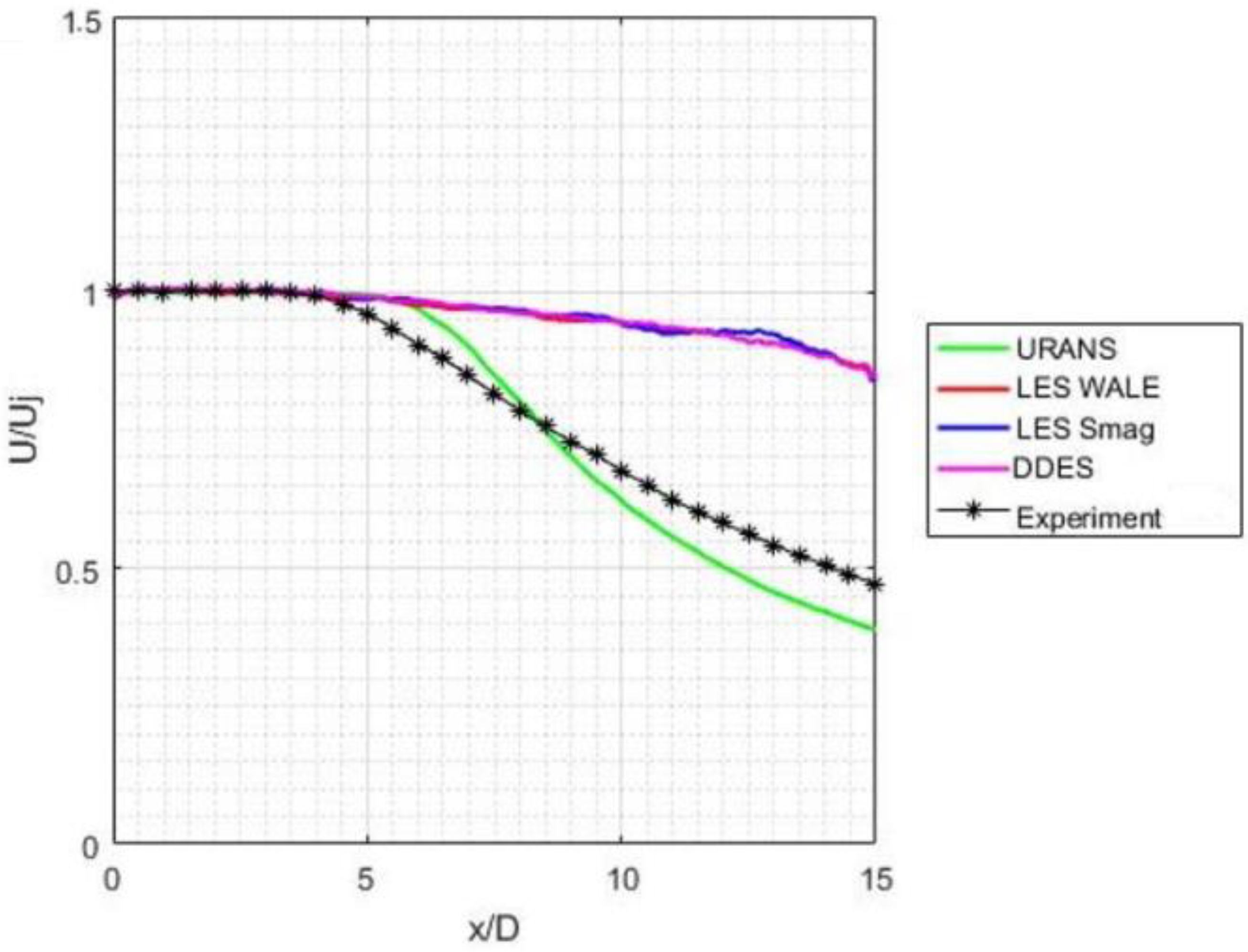
3.1. Centreline Velocity

In Figure 5, the centerline velocity predictions of the various models are compared with the experimental data of the centerline velocity (non-dimensionalized with exit jet velocity, U_j). Figure 6 shows the predictions of different turbulent models compared with the experimental data of Sharma and Nikam [19]. While all models reproduce the experimental data in the near field, the LES and the DES models are found to over-predict the centerline velocity beyond x/D = 5.5. This inaccuracy can be attributed to the uncertainties in the inflow conditions, which poorly predict the initial shear layer (commonly one order of magnitude thicker than what is found experimentally). Since the resolution of the initial shear layer is strongly coupled with the centerline evolution of mean and fluctuating components of axial velocity, the potential core length prediction will be unreliable unless sufficiently thin initial shear layers are used. Bodony and Lele [18] and Wang et al. [39] have found that a lower-order code overpredicts the potential core length by 200% and the spreading rate by 15% for a round jet from a conventional nozzle.

3.2. Potential Core Length

Potential core length is the non-dimensionalized length at which the U/U_j reduces to 0.95 from 1.00 (Mendez et al. [34]). The potential core length is compared with the experimental data of Sharma and Nikam [29] in Figure 6. It can be clearly seen that the LES-WALE, LES-Smagorinsky, and DDES models have over-predicted the potential core length, whereas the URANS prediction is reasonably good. This is consistent with the observations made with regard to the centreline velocity. Bodony and Lele [18] have also reported the inaccuracy of potential core prediction by LES models as applied to compressible jets—their study was confined to conventional round jets. The present analysis shows such variations (from measurements) in the simulation of the potential core of chevron nozzles as well.

3.3. Velocity Field

The velocity fields predicted by the various models are compared with the experimental images in Figure 7 at two radial planes in the near-field of the jet exit. Figure 7a shows the velocity contours at x/D = 0.5 and Figure 7b shows those at x/D = 2. It can be seen that at x/D = 0.5, the relatively sharper profiles of the shear layer, as predicted by the LES and the DDES models, depict the troughs and the crests of the chevrons closely resembling the experimental contours. At the downstream location (x/D = 2), the cross-section of the jet approaches that of an axisymmetric jet due to the intense mixing caused by the chevrons. Mixing causes the rapid decay of the azimuthal variations in the velocity field. While the gradients within the shear layer tend to get smeared in the URANS profile, the eddy simulation models are able to retain the shear layer structure more evidently (Figure 7b). Since the mixing enhancement is directly related to the acoustics, this observation is important from the perspective of prediction of the acoustics characteristics as well.

The axial velocity contours (which demonstrate the development of the jet along the axis) are shown in Figure 8. The difference in predictions of the potential core by the URANS and the eddy simulation models is clear from the field contours. From the perspective of noise prediction, the evolution of the shear layer and the rate of mixing are more important, which can be inferred from the RMS velocity field shown in Figure 9. Models that simulate the eddies do capture the fluctuations along the jet length, whereas in the URANS modelling the values average to zero except at locations very close to the nozzle exit. This contributes to the discrepancy in prediction of the acoustic properties as well, in the averaged Reynolds stress approach. Results of the eddy simulation methods show that the RMS velocity fluctuations are low in the near field and increase along the axis. This is indicative of the growth of turbulence along the jet. The shear layer regions are characterized by peak values of RMS velocity. This is predicted well by the LES-Smagorinsky model.

In Figure 10, the RMS pressure fluctuations are shown along the axis of the jet. Since sound is a small perturbation of pressure over a mean pressure, the root mean square value of static pressure is directly indicative of the intensity of the acoustic field. While the URANS approach does not model the fluctuations along the jet, the eddy simulation methods capture the fluctuations, and this contributes to the prediction of the sound level. Higher values of RMS pressure stem from significantly higher unsteadiness and an increased level of turbulence.

3.4. OASPL—Acoustic Properties

Seven receivers were kept at a radial distance of 45D with a polar angle(θ) starting from 30° to 90° (in increments of 10°). These were the locations specified by Nikam and Sharma [29] as shown in Figure 2. OASPL was obtained by using FFT (Fast Fourier Transform) of the sound signal. OASPL was computed for all the receiver locations. Figure 11 shows the OASPL variation with receivers located at different polar angles. Comparison with experimental data shows that the LES-Smagorinsky model predicted the qualitative trend as well as the absolute values more accurately than the other turbulent models. LES-WALE predicted the trend accurately, though it has a 2 dB offset at higher polar angles. DES could predict the trend correctly, but the OASPL is underpredicted with an offset of 2.5 dB to 3.5 dB. It can be noted that the accuracy of prediction of the noise level by the eddy simulation approach, in general, is significantly better than that of the URANS approach. The URANS model severely underpredicts the acoustic property. Even the qualitative variation was not captured adequately.

The increase in noise level at lower polar angles (say at 30°) in comparison to that at a polar angle of 90° can be noted in the experimental data. Sharma and Nikam [29] attribute this to the directivity of the source. Both LES and DDES are able to capture this trend in the simulation.

3.5. A Note on the Computational Time

The efficacy of acoustic modelling of the eddy simulation models needs to be evaluated along with the consideration of the computational intensity associated with them. In the present study, the URANS computations took 2.5 h to complete while the eddy simulation models ran for about 120 h on a 192-core machine.

4. Conclusions

The complex jet structure of the chevron nozzle in the compressible flow regime was analyzed using URANS and eddy simulation models, the emphasis being on a critical comparison of the methods in modeling the acoustic field. The two variants of the LES model considered in the present study (Smagorinsky–Lilly and WALE models) predicted the sound pressure level with fairly good accuracy, considering the complexity of the flow field. The detached eddy simulation model was also reasonably accurate in modeling the acoustics. Though the URANS model predicted the jet velocity field with good accuracy, it was not capable of modeling the acoustics accurately. The sound pressure levels as predicted by the Smagorinsky model were particularly in agreement with the experimental data.

The study contributes to the analysis of noise suppression using chevron nozzles by providing a critical evaluation of the performance of the URANS and the eddy simulation models. Comparison of the axial distribution of root mean square pressure of the compressible jet as predicted by the URANS and the eddy simulation models is one of the accomplishments of the study. In view of the applications of this nozzle geometry, the prediction of pressure fluctuations is particularly important. The study also highlights the remarkable improvement in the sound pressure level distributions accomplished by the eddy simulation methods (over the URANS approach) for the characteristically non-axisymmetric compressible jet. Further analysis using the LES and the DES approach can shed more light on the process of mixing enhancement and noise suppression by the chevrons. Geometry optimization of the nozzle with an emphasis on acoustics is an important area that can be immensely benefited by further numerical modeling studies.

References

1. Gjestland, T. A systematic review of the basis for WHO’s new recommendation for limiting aircraft noise annoyance. Int. J. Environ. Res. Public Health 2018, 15, 2717. [Google Scholar] [CrossRef]
2. Blandeau, V.P.; Regnier, V.; Bousquet, P. Acoustic behaviour of ground plates for aircraft noise flight tests. In Proceedings of the 2018 AIAA/CEAS Aeroacoustics Conference, Atlanta, GA, USA, 25–29 June 2018; p. 3295. [Google Scholar]
3. Viswanathan, K. Progress in prediction of jet noise and quantification of aircraft/engine noise components. Int. J. Aeroacoustics 2018, 17, 339–379. [Google Scholar] [CrossRef]
4. Bridges, J.; Wernet, M.; Brown, C. Control of Jet Noise through Mixing Enhancement; 2003. NASA Report No. NASA/TM-2003-212335. Available online: https://ntrs.nasa.gov/citations/20030063290 (accessed on 4 August 2022).
5. Kajikawa, Y.; Gan, W.-S.; Kuo, S.M. Recent advances on active noise control: Open issues and innovative applications. APSIPA Trans. Signal Inf. Process. 2012, 1, 1–21. [Google Scholar] [CrossRef]
6. Stevens, J.; Ahuja, K. Recent advances in active noise control. AIAA J. 1991, 29, 1058–1067. [Google Scholar] [CrossRef]
7. Nikam, S.R.; Sharma, S.D. Effect of a chevron nozzle on noise radiation from a compressible jet. AIAA J. 2018, 56, 4361–4378. [Google Scholar] [CrossRef]
8. Nikam, S.R.; Sharma, S.D. Effect of chevron nozzle penetration on aero-acoustic characteristics of jet at M = 0.8. Fluid Dyn. Res. 2017, 49, 065506. [Google Scholar] [CrossRef]
9. Harish Subramanian, G.; Nagarjun, C.H.; Satish Kumar, K.V.; Ashish Kumar, B.; Srikanth, V.; Srikrishnan, A.R. Mixing enhancement using chevron nozzle: Studies on free jets and confined jets. Sādhanā 2018, 43, 1–14. [Google Scholar] [CrossRef]
10. Bridges, J.; Brown, C. Parametric testing of chevrons on single flow hot jets. In Proceedings of the 10th AIAA/CEAS Aeroacoustics Conference, NASA, Cleveland, OH, USA, 10–12 May 2004; p. 2824. [Google Scholar]
11. Zaman, K.; Bridges, J.E.; Huff, D.L. Evolution from ‘tabs’ to ‘chevron technology’—A review. Int. J. Aeroacoustics 2011, 10, 685–709. [Google Scholar] [CrossRef]
12. Callender, B.; Gutmark, E.; Martens, S. Far-field acoustic investigation into chevron nozzle mechanisms and trends. AIAA J. 2005, 43, 87–95. [Google Scholar] [CrossRef]
13. Murugesan, P.; Kumar, A.B.; Kambhampati, A.T.; Pillai, S.; Chandrasekar, G.C.; Raghavannambiar, S.A.; Velamati, R.K. Numerical Study of Characteristics of Underexpanded Supersonic Jet. J. Aerosp. Technol. Manag. 2020, 12, 1126. [Google Scholar]
14. Sudhan, K.H.; Prasad, G.K.; Kothurkar, N.K.; Srikrishnan, A.R. Studies on supersonic cold spray deposition of microparticles using a bell-type nozzle. Surf. Coat. Technol. 2020, 383, 125244. [Google Scholar] [CrossRef]
15. Tide, P.S.; Babu, V. Numerical predictions of noise due to subsonic jets from nozzles with and without chevrons. Appl. Acoust. 2009, 70, 321–332. [Google Scholar] [CrossRef]
16. Lew, P.-T.; Blaisdell, G.; Lyrintzis, A. Recent progress of hot jet aeroacoustics using 3-D large-eddy simulation. In Proceedings of the 11th AIAA/CEAS Aeroacoustics Conference, Purdue University, West Lafayette, IN, USA, 23–25 May 2005; p. 3084. [Google Scholar]
17. Bodony, D.; Lele, S. Generation of low frequency sound in turbulent jets. In Proceedings of the 11th AIAA/CEAS Aeroacoustics Conference, Sanford University, Sanford, FL, USA, 23–25 May 2005; p. 3041. [Google Scholar]
18. Bodony, D.J.; Lele, S.K. Current status of jet noise predictions using large-eddy simulation. AIAA J. 2008, 46, 364–380. [Google Scholar] [CrossRef]
19. Dawi, A.H.; Akkermans, R.A. Spurious noise in direct noise computation with a finite volume method for automotive applications. Int. J. Heat Fluid Flow 2018, 72, 243–256. [Google Scholar] [CrossRef]
20. Dawi, A.H.; Akkermans, R.A. Direct noise computation of a generic vehicle model using a finite volume method. Comput. Fluids 2019, 191, 104243. [Google Scholar] [CrossRef]
21. Depuru Mohan, N.K.; Dowling, A.P. Jet-noise-prediction model for chevrons and microjets. AIAA J. 2016, 54, 3928–3940. [Google Scholar] [CrossRef]
22. Andersson, N.; Eriksson, L.-E.; Davidson, L. Large-eddy simulation of a Mach 0.75 jet. In Proceedings of the 9th AIAA/CEAS Aeroacoustics Conference and Exhibit, Chalmers University of Technology, Gotenborg, Sweden, 12–14 May 2003; p. 3312. [Google Scholar]
23. Andersson, N.; Eriksson, L.-E.; Davidson, L. A study of Mach 0.75 jets and their radiated sound using large-eddy simulation. In Proceedings of the 10th AIAA/CEAS Aeroacoustics Conference and Exhibit, Chalmers University of Technology, Gotenborg, Sweden, 10–12 May 2004; p. 3024. [Google Scholar]
24. Andersson, N.; Eriksson, L.-E.; Davidson, L. Investigation of an isothermal Mach 0.75 jet and its radiated sound using large-eddy simulation and Kirchhoff surface integration. Int. J. Heat Fluid Flow 2005, 26, 393–410. [Google Scholar] [CrossRef]
25. Engblom, W.; Khavaran, A.; Bridges, J. Numerical prediction of chevron nozzle noise reduction using WIND-MGBK methodology. In Proceedings of the 10th AIAA/CEAS Aeroacoustics Conference, NASA, Cleveland, OH, USA, 10–12 May 2004; p. 2979. [Google Scholar]
26. Papadrakakis, M.; Papadopoulos, V.; Stefanou, G.; Plevris, V. On the Simulation of Aerodynamic Noise With Different Turbulence Models. In Proceedings of the ECCOMASS Congress, Technische Universitat Darmstadt, Darmstadt, Germany, 5–10 June 2016. [Google Scholar]
27. Han, X.; Jin, Y.; Fan, P. Compressibility Modified RANS Simulations for Noise Prediction of Jet Exhausts with Chevron. J. Appl. Fluid Mech. 2020, 14, 793–804. [Google Scholar]
28. Sarkar, S. The pressure—Dilatation correlation in compressible flows. Phys. Fluids A Fluid Dyn. 1992, 4, 2674–2682. [Google Scholar] [CrossRef]
29. Nikam, S.R.; Sharma, S.D. Aero-acoustic Characteristics of Compressible Jets from Chevron Nozzle. In Proceedings of the 20th AIAA/CEAS Aeroacoustics Conference IIT Bombay, Atlanta, GA, USA, 16–20 June 2014; p. 2623. [Google Scholar]
30. Menter, F. Zonal two equation kw turbulence models for aerodynamic flows. In Proceedings of the 23rd Fluid Dynamics, Plasmadynamics, and Lasers Conference, Orlando, FL, USA, 6–9 July 1993. [Google Scholar]
31. Fröhlich, J.; Von Terzi, D. Hybrid LES/RANS methods for the simulation of turbulent flows. Prog. Aerosp. Sci. 2008, 44, 349–377. [Google Scholar] [CrossRef]
32. ANSYS. ANSYS Fluent Theory Guide, Release 19.0.; ANSYS, Inc.: Canonsburg, PA, USA, 2019. [Google Scholar]
33. Ben-Nasr, O.; Hadjadj, A.; Chaudhuri, A.; Shadloo, M.S. Assessment of subgrid-scale modeling for large-eddy simulation of a spatially-evolving compressible turbulent boundary layer. Comput. Fluids 2017, 151, 144–158. [Google Scholar] [CrossRef]
34. Mendez, S.; Shoeybi, M.; Lele, S.K.; Moin, P. On the use of the Ffowcs Williams-Hawkings equation to predict far-field jet noise from large-eddy simulations. Int. J. Aeroacoustics 2013, 12, 1–20. [Google Scholar] [CrossRef]
35. Ffowcs Williams, J.E.; Hawkings, D.L. Sound generation by turbulence and surfaces in arbitrary motion. Philos. Trans. R. Soc. Lond. Ser. A Math. Phys. Sci. 1969, 264, 321–342. [Google Scholar]
36. Spalart, P.R.; Deck, S.; Shur, M.L.; Squires, K.D.; Strelets, M.K.; Travin, A. A new version of detached-eddy simulation, resistant to ambiguous grid densities. Theor. Comput. Fluid Dyn. 2006, 20, 181–195. [Google Scholar] [CrossRef]
37. Gritskevich, M.S.; Garbaruk, A.V.; Schütze, J.; Menter, F.R. Development of DDES and IDDES formulations for the k-ω shear stress transport model. Flow Turbul. Combust. 2012, 88, 431–449. [Google Scholar] [CrossRef]
38. Mockett, C.; Fuchs, M.; Garbaruk, A.; Shur, M.; Spalart, P.; Strelets, M.; Thiele, F.; Travin, A. Two non-zonal approaches to accelerate RANS to LES transition of free shear layers in DES. In Progress in Hybrid RANS-LES Modelling; Springer: Berlin/Heidelberg, Germany, 2015; pp. 187–201. [Google Scholar]
39. Wang, Z.; Ameen, M.M.; Som, S.; Abraham, J. Assessment of Large-Eddy Simulations of Turbulent Round Jets Using Low-Order Numerical Schemes. SAE Int. J. Commer. Veh. 2017, 10, 572–581. [Google Scholar] [CrossRef]
Figure 1. Cut section of chevron nozzle showing geometric details. (Reprinted/adapted with permission from Ref. [29]. 2014, Nikam, S.R. and Sharma, S.D.)
Symmetry 14 01975 g001
Figure 2. Details of computational grid used in the present study. (a) Various volumetric regions defined for fine mesh close to the nozzle; (b) closer view of mid plane grid showing finer grid near the exit of chevron nozzle; (c) mesh in mid plane showing gradually varying grid size.
Symmetry 14 01975 g002aSymmetry 14 01975 g002b
Figure 3. FWH-surface (marked by black lines) enclosing the entire turbulent region (contours of turbulent kinetic energy, m2/s2).
Symmetry 14 01975 g003
Figure 4. Receivers locations as in the experiment of Nikam and Sharma. (Reprinted/adapted with permission from Ref. [29]. 2014, Nikam, S.R. and Sharma, S.D.).
Symmetry 14 01975 g004
Figure 5. Non-dimensionalized centerline velocity, compared with the measurements of Sharma and Nikam [29].
Symmetry 14 01975 g005
Figure 6. Comparison of potential core length of turbulence models with experimental data [29].
Symmetry 14 01975 g006
Figure 7. (a). Velocity field at x/D = 0.5; (b). Velocity field at x/D = 2.
Symmetry 14 01975 g007
Figure 8. Axial velocity field as predicted by the various models.
Symmetry 14 01975 g008
Figure 9. Root Mean Square (RMS) velocity field as predicted by the various models.
Symmetry 14 01975 g009
Figure 10. Root Mean Square (RMS) pressure along the axis as predicted by the various models.
Symmetry 14 01975 g010
Figure 11. OASPL vs. polar angles, comparison with the experiment of Nikam and Sharma [29].
Symmetry 14 01975 g011
Publisher’s Note: MDPI stays neutral with regard to jurisdictional claims in published maps and institutional affiliations.