Hamming Similarity Programming Model for Multi-Attribute Decision-Making Objects with Attribute Values as Interval Numbers and Its Application

Abstract

With regard to the interval number-based uncertain multi-attribute decision making problem, in which the attribute weights are unknown and there is no preference on decision-making alternative objects, this paper presents a new decision-making approach. In this method, Hamming distance firstly is used to define the Hamming similarity degree of normative interval numbers, and the Hamming similarity degree of decision-making alternative objects, and then the Hamming similarity superiority relation theory to the comparison of interval numbers is proposed and some relevant results are obtained. Thus, by drawing on the idea of deviations maximization, an interval number-based decision-making object Hamming similarity programming model (IN-DMOHSPM) is established to calculate and solve the weight vector of attributes. Next, all of the selected alternative objects set is screened and sorted by using the overall Hamming similarity degree of each decision-making object compared with the ideal optimal object, and a new algorithm of Hamming similarity programming model for interval number-based multiple attribute decision-making objects is presented. Finally, the feasibility and utility of this model used in this paper are demonstrated by a numerical example.

1. Introduction

Uncertain multi-attribute decision making (UMADM) is also known as uncertain multi-objective decision making with a finite scheme [1,2]. It is a significant component of the study of modern decision-making science theories and methods, and widely exists in many practical problems, such as urban industrial planning, logistics network economy, organizational and environmental performance, quality and benefits estimation, public transport network design, centralized distribution network optimization, pattern matching and intelligent control. Its theories and methods have been widely explored and applied, such as the best matching evaluation of manufacturing technology and product specifications [3], the multidimensional evaluation of organizational performance [4], the environmental performance evaluation of the cross-efficiency DEA (data envelopment analysis, DEA) model [5], the environmental biased technical progress measurement evaluation considering energy conservation and emission reduction [6], the evaluation of China’s industrial green technology and its effect on energy conservation and emission reduction [7], the optimization of urban emission reduction and energy conservation efficiency calculation [8], airport centralized distribution network optimization [9], agent simulation bus line network design [10], dynamic multi-attribute group emergency decision making considering experts’ hesitation [11], gray correlation analysis of weapon system modularization priority [12] and other application practice fields. It should be noted that in the process of understanding some fuzzy things, especially things in development and under change, people are often affected by the subjectivity, limitations, preferences and other uncertain information of thinking judgment, and will not only focus on or stay on any exact or fixed numerical information. In real life, because of the complexity and objectivity of decision-making problems, the fuzziness of human thinking and the incompleteness and nondeterminacy of decision-making information, expressing the objective information and their preferences with accurate numerical values is tough for people. They often use interval number values, triangular fuzzy number values or linguistic values that are more consistent with the objective reality to quantify the information of things and the information processing process. This can effectively overcome the uncertainty of the decision-making value caused by the fuzziness of information. Therefore, the similarity measure [13] provides an important basic tool and approach for people to conduct analogical logic reasoning on two or more things with uncertain fuzzy concepts. Research on many uncertain decision-making problems relies on the application of the similarity measure, such as prediction [14], expectation [15], optimization [16], evaluation [17], random simulation [18], matrix game [19] and spatial representation [20]. So, it is vital to find a scientific, simple and reasonable ranking algorithm to improve the decision-making efficiency. At present, common ranking methods for UMADM problems with unknown attribute weights and no preference for decision-making objects include the following in

Table 1. Common ranking method.

Author	Year	Method	Application
Zhang, L.Y. et al. [13]	2013	Similarity measurement	TFNs information and MCGDM
Xu, Z.S. and Da, Q.L. [21]	2005	Minimum deviation method	Priorities of fuzzy preference matrix
Saaty T.L. [22]	1980	Feature vector method	Analytic hierarchy process
Gou, G.L. and Wang, G.Y. [23]	2016	Incremental updating approximations	Confidential dominance relation based rough set
Ju, Y.B. and Wang, A.H. [24]	2013	Extension of VIKOR	MCGDM problem with linguistic information
Sevastianov P. [25]	2007	Probabilistic approach and Dempster–Shafer theory	Interval and fuzzy number comparison
Huang, Z.L. and Luo, J. [26]	2019	Relative similarity relation method	UMCDM with criteria values as interval number
Huang, Z.L. and Luo, J. [27]	2017	Possibility degree programming model	UMADM with attribute values as interval number
Huang, Z.L et al. [28]	2012	Prospect theory model	MCDM with alternative values as interval number
Liu, Y. et al. [29]	2013	Grey target based on prospect theory	Multi-objective grey target decision-making
Sun, Y. et al. [30]	2017	Relative dominance relation method	MADM based on weights aggregation
Zhang, X.X. and Wang, Y.M. [31]	2019	Interval belief structure	Hybrid Multi-attribute decision making
Ding, Q.Y. et al. [32]	2021	Interval-value hesitation fuzzy TODIM	TODIM for dynamic emergency responses
Lai, L.B. et al. [33]	2019	Graph cooperative game method	Game Theory and Graph cooperative game with interval-valued payoffs

.

The determination of attribute weight occupies an important position in UMADM-related research. It is not difficult to point out that many experts and scholars are used to using traditional methods such as the maximizing deviation method [34], the improved maximizing deviation method [35], the information entropy method [36], the relative similarity programming model algorithm [37] and the quadratic programming-based relative superiority method [38] to determine the attribute weight, and then collect relevant decision-making information in combination with their own characteristics and then select and rank the best. These methods have achieved obvious results in the measurement and ranking of the advantages and disadvantages of the decision objects. It is often encountered that the indicator attribute values are similar to the measurement values, the large similarity and small difference of the evaluation results of the scheme objects are evident and the low overall discrimination of the final decision level is evident, which easily leads to the distortion of the decision results in the application process of dealing with the UMADM problem. Although the traditional classical deviation maximization weighting algorithm can effectively amplify the difference between the measured values of the indicator attributes among the selected decision-making objects, and is more convenient for the measurement, screening and ranking of the pros and cons of the scheme objects, it simply contains the impact of the difference information between the measured values of the initial indicator attributes on the decision-making results. However, it fails to take into account the impact of the similarity measurement [13] information between the measured values of the indicator attributes on the indicator attributes themselves in the evaluation process of incomplete information systems such as UMADM [39,40], which is easy to cause the judgment and ranking of the quality of the selected decision-making object set to be inconsistent with the actual situation.

Therefore, in order to overcome the problems encountered above, for the interval number-based uncertain multiple attribute decision-making (IN-UMADM) problem where attribute weights are unknown with no preference for decision-making objects, this paper give new formulas for the definition of Hamming similarity degree of the normalized interval number and Hamming similarity degree of the decision-making objects by using the Hamming distance [41,42], and the related property results of the dominance relation theory to comparative Hamming similarity degree for interval numbers (i.e., there is an equivalent relationship between the Hamming similarity degree size of each offered alternative object with the ideal alternative object and the dominance size of each offered decision-making alternative object). Taking into account the role of Hamming similarity degree between the measurement data of attributes in the UMADM problem, a new Hamming similarity programming model is designed and constructed to obtain a more realistic weighting assignment equation for attributes based on the Hamming similarity relationship between interval number-based attribute values. After the aggregation and fusion of alternative decision information, the differences of similarity degree among all the selected alternative objects will be reduced, that is, the differences among the selected alternative objects will be expanded, which is conducive to the identification of the advantages and disadvantages of the selected alternative objects and the screening and sorting. At last, the overall Hamming similarity degree of each alternative decision object compared with the ideal alternative decision object is used to screen and rank all of the selected alternative object set, and a new algorithm of the Hamming similarity programming model for interval number-based multiple attribute decision-making objects is presented.

2. Superiority Relation Theories to Compare Hamming Similarity Degree for Interval Numbers

2.1. Hamming Similarity Degree for Interval Numbers

Definition 1.

If $\tilde{x}=\left[x^L,x^U\right]=\left\{x\right|x^L\le x\le x^U,x^L,x^U\in R\}$, $\tilde{x}$is called an interval number [1,2,26,27,28] (IN), where $x^L$ and $x^U$are the lower and upper bounds supported by interval number $\tilde{x}$, which are generally called small elements and large elements. In particular, if the interval number $\tilde{x}=\left[x^L,x^U\right]$also satisfies $0<x^L\le x^U<1$, then $\tilde{x}$is called to be a normalized interval number. If $x^L=x^U$,$\tilde{x}$degenerates into a real number, that is, $\tilde{x}=x^L=x^U$, we denote $l_{\tilde{x}}=x^U-x^L$as the width of the interval number $\tilde{x}$, when $l_{\tilde{x}}=0$, and $\tilde{x}$is also a real number.

For the convenience of the following analysis, the operation rules about interval numbers are first given as follows: Let $\tilde{x}=\left[x^L,x^U\right]$, $\tilde{y}=\left[y^L,y^U\right]$, and then we have

Rule 1 $\tilde{x}+\tilde{y}=\left[x^L+y^L,x^U+y^U\right]$;

Rule 2 $\tilde{x}-\tilde{y}=\left[x^L-y^U,x^U-y^L\right]$;

Rule 3 $\frac{1}{\tilde{x}}=\left[\frac{1}{x^U},\frac{1}{x^L}\right],x^L,x^U>0 \mathrm{or} x^L,x^U<0$;

Rule 4$k\tilde{x}=\left[k{x}^L,k{x}^U\right]$, where $k>0$, in particular, if $k=0$, then $k\tilde{x}=0$; $k\tilde{x}=\left[k{x}^U,k{x}^L\right]$, where $k<0$;

Rule 5 If and only if $x^L=y^L$, $x^U=y^U$, then $\tilde{x}=\tilde{y}$.

To introduce the definition of Hamming similarity, we first define the concept of Hamming divergence of interval numbers using the Hamming distance [41,42] (Hamming distance).

Definition 2.

Let two arbitrary normalized interval numbers $\tilde{x}=\left[x^L,x^U\right]$and $\tilde{y}=\left[y^L,y^U\right]$, if norm

$${\parallel \tilde{x}-\tilde{y}\parallel }_{IN}=\left|x^L-y^L\right|+\left|x^U-y^U\right|.$$

(1)

Then, $d_{IN}\left(\tilde{x},\tilde{y}\right)=\tilde{x}-{\tilde{y}}_{IN}$is called the Hamming deviation degree [27,28] between normalized interval numbers $\tilde{x}$ and $\tilde{y}$. Obviously, the larger the $d_{IN}\left(\tilde{x},\tilde{y}\right)$ value is, the greater the degree of separation between $\tilde{x}$ and $\tilde{y}$ from each other. In particular, when $d_{IN}\left(\tilde{x},\tilde{y}\right)=0$, then $\tilde{x}=\tilde{y}$, i.e., $\tilde{x}$ and $\tilde{y}$ are equal.

Definition 3.

Let two arbitrary normalized interval numbers $\tilde{x}=\left[x^L,x^U\right]$and $\tilde{y}=\left[y^L,y^U\right]$, then

$$s_{IN}\left(\tilde{x},\tilde{y}\right)=1-\frac{\left|x^L-y^L\right|+\left|x^U-y^U\right|}{2}=1-\frac{1}{2}{d}_{IN}\left(\tilde{x},\tilde{y}\right),$$

(2)

where $s_{IN}\left(\tilde{x},\tilde{y}\right)$is called the Hamming similarity degree between normalized interval numbers $\tilde{x}$and $\tilde{y}$[2,39,40]. It is easy to know that the larger the$s_{IN}\left(\tilde{x},\tilde{y}\right)$value, the greater the degree of similarity between $\tilde{x}$and $\tilde{y}$. In particular, when$s_{IN}\left(\tilde{x},\tilde{y}\right)=1$, there is $\tilde{x}=\tilde{y}$, i.e., the interval number$\tilde{x}$is completely similar to$\tilde{y}$.

From the definition of Hamming similarity degree for normalized interval numbers given in Definition 3 above, the following properties are easily obtained.

Theorem 1.

Let any given three normalized interval numbers be set as $\tilde{x}=\left[x^L,x^U\right]$, $\tilde{y}=\left[y^L,y^U\right]$and $\tilde{z}=\left[z^L,z^U\right]$, then, we have the following:

(1)

Boundedness, $0\le s_{IN}\left(\tilde{x},\tilde{y}\right)\le 1;$

(2)

Self-reflexivity, $s_{IN}\left(\tilde{x},\tilde{x}\right)=1;$

(3)

Symmetry, $s_{IN}\left(\tilde{x},\tilde{y}\right)=s_{IN}\left(\tilde{y},\tilde{x}\right);$

(4)

Transitivity, if $s_{IN}\left(\tilde{x},\tilde{y}\right)=1$, $s_{IN}\left(\tilde{y},\tilde{z}\right)=1$then $s_{IN}\left(\tilde{x},\tilde{z}\right)=1$, that is, if $\tilde{x}$is exactly similar to $\tilde{y}$and $\tilde{y}$is exactly similar to $\tilde{z}$, then $\tilde{x}$is exactly similar to $\tilde{z}$.

(5)

Proximity, if $s_{IN}\left(\tilde{x},\tilde{y}\right)\le s_{IN}\left(\tilde{x},\tilde{z}\right).$, then $\tilde{z}$is said to be closer to $\tilde{x}$than $\tilde{y}$; if $s_{IN}\left(\tilde{x},\tilde{y}\right)\le s_{IN}\left(\tilde{z},\tilde{y}\right)$, then $\tilde{z}$is said to be closer to $\tilde{y}$than $\tilde{x}$.

According to the definition of interval number Hamming similarity, it is easy to prove that the conclusion of Theorem 1 is valid. The proof process is omitted.

Definition 4.

Let the alternative decision-making objects composed of the sequence of normal interval numbers be set as$X=\left\{{\tilde{x}}_1,{\tilde{x}}_2,\cdots ,{\tilde{x}}_m\right\}$and$Y=\left\{{\tilde{y}}_1,{\tilde{y}}_2,\cdots ,{\tilde{y}}_m\right\}.$ Then,

$$S_{IN}\left(X,Y\right)=\frac{1}{m}{\sum }_{i=1}^m{s}_{IN}\left({\tilde{x}}_i,{\tilde{y}}_i\right)=1-\frac{1}{2m}{\sum }_{i=1}^m{d}_{IN}\left({\tilde{x}}_i,{\tilde{y}}_i\right),$$

(3)

where $S_{IN}\left(X,Y\right)$is called the Hamming similarity degree between decision-making objects X and Y.

Suppose the weighted normalized interval number-based decision-making matrix is $\tilde{Z}={({\tilde{z}}_{ij})}_{n\times m}$, where ${\tilde{z}}_{ij}=[z_{ij}^L,z_{ij}^U]$, $i\in N,j\in M$. Then, we have the following definition.

Definition 5.

$Z^{+\ast }=\{{\tilde{z}}_1^{+\ast },{\tilde{z}}_2^{+\ast },\cdots ,{\tilde{z}}_m^{+\ast }\}$is called an interval number-based positive ideal decision-making object composed by a positive ideal points sequence, where

$${\tilde{z}}_j^{+\ast }=[z_j^{+\ast L},z_j^{+\ast U}]=[\underset{i}{max}(z_{ij}^L),\underset{i}{max}(z_{ij}^U)],j=1,2,\cdots ,m,$$

(4)

is a positive ideal point [2,26,27,28] and the larger the value, the better it is.$Z^{-\ast }=\{{\tilde{z}}_1^{-\ast },{\tilde{z}}_2^{-\ast },\cdots ,{\tilde{z}}_m^{-\ast }\}$is called an interval number-based negative ideal decision-making object composed by a negative ideal points sequence, where

$${\tilde{z}}_j^{-\ast }=[z_j^{-\ast L},z_j^{-\ast U}]=[\underset{i}{min}(z_{ij}^L),\underset{i}{min}(z_{ij}^U)],j=1,2,\cdots ,m,$$

(5)

is a negative ideal point [2,26,27,28], and the smaller the value, the worse it is.

2.2. Superiority Relation to Comparing Hamming Similarity Degree for Interval Numbers

According to the concept of Hamming similarity degree already given above, we define the relevant definitions and main results concerning the superiority relation to comparing Hamming similarity degree for normalized interval numbers and interval number sequences as follows:

Definition 6.

Let any two normalized interval numbers be $\tilde{x}=\left[x^L,x^U\right]$and $\tilde{y}=\left[y^L,y^U\right]$and interval number-based positive and negative ideal points be ${\tilde{z}}^{+\ast }=\left[z^{+\ast L},z^{+\ast U}\right]$and ${\tilde{z}}^{-\ast }=\left[z^{-\ast L},z^{-\ast U}\right]$, if

$$s_{IN}(\tilde{x},{\tilde{z}}^{+\ast })>s_{IN}(\tilde{y},{\tilde{z}}^{+\ast })\vee s_{IN}(\tilde{x},{\tilde{z}}^{-\ast })<s_{IN}(\tilde{y},{\tilde{z}}^{-\ast }),$$

(6)

then the normalized interval number $\tilde{x}$is superior compared to $\tilde{y}$[2], which is denoted as:$\tilde{x}\succ \tilde{y}$. Obviously, the larger the Hamming similarity degree with theinterval number-basedpositive ideal point, or the smaller the Hamming similarity degree with theinterval number-basednegative ideal point, the larger the dominance of the corresponding interval number.

Theorem 2.

If and only if the positive and negative ideal points are the optimal decision points for decision making, then

$$\tilde{x}\succ \tilde{y}\iff d_{IN}(\tilde{x},{\tilde{z}}^{+\ast })<d_{IN}(\tilde{y},{\tilde{z}}^{+\ast })\vee d_{IN}(\tilde{x},{\tilde{z}}^{-\ast })>d_{IN}(\tilde{y},{\tilde{z}}^{-\ast })\iff x^L+x^U>y^L+y^U.$$

(7)

Proof. 

Obviously, from Definition 6, it follows that □

$$\tilde{x}\succ \tilde{y}\iff s_{IN}(\tilde{x},{\tilde{z}}^{+\ast })>s_{IN}(\tilde{y},{\tilde{z}}^{+\ast })\vee s_{IN}(\tilde{x},{\tilde{z}}^{-\ast })<s_{IN}(\tilde{y},{\tilde{z}}^{-\ast }).$$

According to Equation (2), we obtain

$$s_{IN}(\tilde{x},{\tilde{z}}^{+\ast })>s_{IN}(\tilde{y},{\tilde{z}}^{+\ast })\vee s_{IN}(\tilde{x},{\tilde{z}}^{-\ast })<s_{IN}(\tilde{y},{\tilde{z}}^{-\ast })\iff$$

$$d_{IN}(\tilde{x},{\tilde{z}}^{+\ast })<d_{IN}(\tilde{y},{\tilde{z}}^{+\ast })\vee d_{IN}(\tilde{x},{\tilde{z}}^{-\ast })>d_{IN}(\tilde{y},{\tilde{z}}^{-\ast }),$$

Therefore,

$$\tilde{x}\succ \tilde{y}\iff d_{IN}(\tilde{x},{\tilde{z}}^{+\ast })<d_{IN}(\tilde{y},{\tilde{z}}^{+\ast })\vee d_{IN}(\tilde{x},{\tilde{z}}^{-\ast })>d_{IN}(\tilde{y},{\tilde{z}}^{-\ast }).$$

Additionally, according to Equation (1), we have

$$d_{IN}(\tilde{x},{\tilde{z}}^{+\ast })=\left|x^L-z^{+\ast L}\right|+\left|x^U-z^{+\ast U}\right|,d_{IN}(\tilde{y},{\tilde{z}}^{+\ast })=\left|y^L-z^{+\ast L}\right|+\left|y^U-z^{+\ast U}\right|,$$

$$d_{IN}(\tilde{x},{\tilde{z}}^{-\ast })=\left|x^L-z^{-\ast L}\right|+\left|x^U-z^{-\ast U}\right|,d_{IN}(\tilde{y},{\tilde{z}}^{-\ast })=\left|y^L-z^{-\ast L}\right|+\left|y^U-z^{-\ast U}\right|;$$

When the positive and negative ideal points are the optimal decision-making points, i.e., ${\tilde{z}}^{+\ast }=\left[z^{+\ast L},z^{+\ast U}\right]$, ${\tilde{z}}^{-\ast }=\left[z^{-\ast L},z^{-\ast U}\right]$ is the interval number-based ideal point, hence, we have

$$z^{+\ast L}\ge max\left\{x^L,y^L\right\},z^{+\ast U}\ge max\left\{x^U,y^U\right\},z^{-\ast L}\le min\left\{x^L,y^L\right\},z^{-\ast U}\le min\left\{x^U,y^U\right\}.$$

Then, we can obtain

$$d_{IN}\left(\tilde{x},{\tilde{z}}^{+\ast }\right)=\left(z^{+\ast L}+z^{+\ast U}\right)-\left(x^L+x^U\right),d_{IN}\left(\tilde{y},{\tilde{z}}^{+\ast }\right)=\left(z^{+\ast L}+z^{+\ast U}\right)-\left(y^L+y^U\right),$$

$$d_{IN}\left(\tilde{x},{\tilde{z}}^{-\ast }\right)=\left(x^L+x^U\right)-\left(z^{-\ast L}+z^{-\ast U}\right),d_{IN}\left(\tilde{y},{\tilde{z}}^{-\ast }\right)=\left(y^L+y^U\right)-\left(z^{-\ast L}+z^{-\ast U}\right);$$

As

$$d_{IN}\left(\tilde{x},{\tilde{z}}^{+\ast }\right)<d_{IN}\left(\tilde{y},{\tilde{z}}^{+\ast }\right)\vee d_{IN}\left(\tilde{x},{\tilde{z}}^{-\ast }\right)>d_{IN}\left(\tilde{y},{\tilde{z}}^{-\ast }\right),$$

Therefore,

$$\tilde{x}\succ \tilde{y}\iff x^L+x^U>y^L+y^U,$$

Thus, the formula (7) holds. Proof is completed.

In the process of judging the dominance relationship between interval numbers, it can be judged directly by using Theorem 2, that is, through computing the Hamming similarity degree value and Hamming deviation degree value between interval numbers with ideal points, or through computing the sum sizes of small and large elements of interval numbers-based attribute values.

Definition 7.

Let alternative decision-making objects composed of the normalized interval number sequence be $X=\left\{{\tilde{x}}_1,{\tilde{x}}_2,\cdots ,{\tilde{x}}_m\right\}$and $Y=\left\{{\tilde{y}}_1,{\tilde{y}}_2,\cdots ,{\tilde{y}}_m\right\}$, and the interval number-based positive and negative ideal decision-making objects composed of positive and negative ideal point sequences be $Z^{+\ast }=\left\{{\tilde{z}}_1^{+\ast },{\tilde{z}}_2^{+\ast },\cdots ,{\tilde{z}}_m^{+\ast }\right\}$and $Z^{-\ast }=\{{\tilde{z}}_1^{-\ast },{\tilde{z}}_2^{-\ast },\cdots ,$${\tilde{z}}_m^{-\ast }\}$, where ${\tilde{x}}_j=[x_j^L,x_j^U]$, ${\tilde{y}}_j=[y_j^L,y_j^U]$, ${\tilde{z}}_j^{+\ast }=[z_j^{+\ast L},z_j^{+\ast U}]$, ${\tilde{z}}_j^{-\ast }=[z_j^{-\ast L},z_j^{-\ast U}]$, $j=1,2,\cdots ,m$, if

$$S_{IN}\left(X,Z^{+\ast }\right)>S_{IN}\left(Y,Z^{+\ast }\right)\vee S_{IN}\left(X,Z^{-\ast }\right)<S_{IN}\left(Y,Z^{-\ast }\right),$$

(8)

then the alternative decision-making object X is superior to Y [2], which is denoted as $X\succ Y$. Obviously, the greater the Hamming similarity degree with the interval number-based positive ideal decision-making object or the smaller the Hamming similarity degree with interval number-based negative ideal decision-making object, the greater the superiority of the corresponding decision-making object.

Theorem 3.

If and only if the interval number-based positive and negative ideal decision-making objects are the optimal object for decision making, then

$$\begin{gathered} X\succ Y\iff {\sum }_{j=1}^m{d}_{IN}\left({\tilde{x}}_j,{\tilde{z}}_j^{+\ast }\right)<{\sum }_{j=1}^m{d}_{IN}\left({\tilde{y}}_j,{\tilde{z}}_j^{+\ast }\right)\vee {\sum }_{j=1}^m{d}_{IN}\left({\tilde{x}}_j,{\tilde{z}}_j^{-\ast }\right)>{\sum }_{j=1}^m{d}_{IN}\left({\tilde{y}}_j,{\tilde{z}}_j^{-\ast }\right)\iff \\ {d}_{IN}\left({\sum }_{j=1}^m{\tilde{x}}_j,{\sum }_{j=1}^m{\tilde{z}}_j^{+\ast }\right)<d_{IN}\left({\sum }_{j=1}^m{\tilde{y}}_j,{\sum }_{j=1}^m{\tilde{z}}_j^{+\ast }\right)\vee d_{IN}\left({\sum }_{j=1}^m{\tilde{x}}_j,{\sum }_{j=1}^m{\tilde{z}}_j^{-\ast }\right)>d_{IN}\left({\sum }_{j=1}^m{\tilde{y}}_j,{\sum }_{j=1}^m{\tilde{z}}_j^{-\ast }\right)\iff {\sum }_{j=1}^m\left(x_j^L+x_j^U\right)> \\ {\sum }_{j=1}^m\left(y_j^L+y_j^U\right). \end{gathered}$$

(9)

Proof. 

Obviously, from definition 7, it can be known that □

$$X\succ Y\iff S_{IN}\left(X,Z^{+\ast }\right)>S_{IN}\left(Y,Z^{+\ast }\right)\vee S_{IN}\left(X,Z^{-\ast }\right)<S_{IN}\left(Y,Z^{-\ast }\right).$$

According to formula (3), it can be obtained that

$$S_{IN}\left(X,Z^{+\ast }\right)>S_{IN}\left(Y,Z^{+\ast }\right)\vee S_{IN}\left(X,Z^{-\ast }\right)<S_{IN}\left(Y,Z^{-\ast }\right)\iff$$

$${\sum }_{j=1}^m{d}_{IN}\left({\tilde{x}}_j,{\tilde{z}}_j^{+\ast }\right)<{\sum }_{j=1}^m{d}_{IN}\left({\tilde{y}}_j,{\tilde{z}}_j^{+\ast }\right)\vee {\sum }_{j=1}^m{d}_{IN}\left({\tilde{x}}_j,{\tilde{z}}_j^{-\ast }\right)>{\sum }_{j=1}^m{d}_{IN}\left({\tilde{y}}_j,{\tilde{z}}_j^{-\ast }\right).$$

Therefore,

$$X\succ Y\iff {\sum }_{j=1}^m{d}_{IN}\left({\tilde{x}}_j,{\tilde{z}}_j^{+\ast }\right)<{\sum }_{j=1}^m{d}_{IN}\left({\tilde{y}}_j,{\tilde{z}}_j^{+\ast }\right)\vee {\sum }_{j=1}^m{d}_{IN}\left({\tilde{x}}_j,{\tilde{z}}_j^{-\ast }\right)>{\sum }_{j=1}^m{d}_{IN}\left({\tilde{y}}_j,{\tilde{z}}_j^{-\ast }\right).$$

According to formula (1), we can obtain

$${\sum }_{j=1}^m{d}_{IN}\left({\tilde{x}}_j,{\tilde{z}}_j^{+\ast }\right)={\sum }_{j=1}^m\left(\left|x_j^L-z_j^{+\ast L}\right|+\left|x_j^U-z_j^{+\ast U}\right|\right),$$

$${\sum }_{j=1}^m{d}_{IN}\left({\tilde{y}}_j,{\tilde{z}}_j^{+\ast }\right)={\sum }_{j=1}^m\left(\left|y_j^L-z_j^{+\ast L}\right|+\left|y_j^U-z_j^{+\ast U}\right|\right),$$

$${\sum }_{j=1}^m{d}_{IN}\left({\tilde{x}}_j,{\tilde{z}}_j^{-\ast }\right)={\sum }_{j=1}^m\left(\left|x_j^L-z_j^{-\ast L}\right|+\left|x_j^U-z_j^{-\ast U}\right|\right),$$

$${\sum }_{j=1}^m{d}_{IN}\left({\tilde{y}}_j,{\tilde{z}}_j^{-\ast }\right)={\sum }_{j=1}^m\left(\left|y_j^L-z_j^{-\ast L}\right|+\left|y_j^U-z_j^{-\ast U}\right|\right),$$

$$d_{IN}\left({\sum }_{j=1}^m{\tilde{x}}_j,{\sum }_{j=1}^m{\tilde{z}}_j^{+\ast }\right)=\left|{\sum }_{j=1}^m{x}_j^L-{\sum }_{j=1}^m{z}_j^{+\ast L}\right|+\left|{\sum }_{j=1}^m{x}_j^U-{\sum }_{j=1}^m{z}_j^{+\ast U}\right|,$$

$$d_{IN}\left({\sum }_{j=1}^m{\tilde{y}}_j,{\sum }_{j=1}^m{\tilde{z}}_j^{+\ast }\right)=\left|{\sum }_{j=1}^m{y}_j^L-{\sum }_{j=1}^m{z}_j^{+\ast L}\right|+\left|{\sum }_{j=1}^m{y}_j^U-{\sum }_{j=1}^m{z}_j^{+\ast U}\right|,$$

$$d_{IN}\left({\sum }_{j=1}^m{\tilde{x}}_j,{\sum }_{j=1}^m{\tilde{z}}_j^{-\ast }\right)=\left|{\sum }_{j=1}^m{x}_j^L-{\sum }_{j=1}^m{z}_j^{-\ast L}\right|+\left|{\sum }_{j=1}^m{x}_j^U-{\sum }_{j=1}^m{z}_j^{-\ast U}\right|,$$

$$d_{IN}\left({\sum }_{j=1}^m{\tilde{y}}_j,{\sum }_{j=1}^m{\tilde{z}}_j^{-\ast }\right)=\left|{\sum }_{j=1}^m{y}_j^L-{\sum }_{j=1}^m{z}_j^{-\ast L}\right|+\left|{\sum }_{j=1}^m{y}_j^U-{\sum }_{j=1}^m{z}_j^{-\ast U}\right|.$$

When the interval number-based positive and negative ideal decision-making objects are the optimal object, that is, $Z^{+\ast }=\left\{{\tilde{z}}_1^{+\ast },{\tilde{z}}_2^{+\ast },\cdots ,{\tilde{z}}_m^{+\ast }\right\}$, $Z^{-\ast }=\left\{{\tilde{z}}_1^{-\ast },{\tilde{z}}_2^{-\ast },\cdots ,{\tilde{z}}_m^{-\ast }\right\}$ is the interval number-based positive and negative ideal sequence composed of positive and negative ideal points, hence, we have

$$z_j^{+\ast L}\ge max\left\{x_j^L,y_j^L\right\},z_j^{+\ast U}\ge max\left\{x_j^U,y_j^U\right\},$$

$$z_j^{-\ast L}\le min\left\{x_j^L,y_j^L\right\},z_j^{-\ast U}\le min\left\{x_j^U,y_j^U\right\},j=1,2,\cdots ,m.$$

So, we can obtain

$${\sum }_{j=1}^m{d}_{IN}\left({\tilde{x}}_j,{\tilde{z}}_j^{+\ast }\right)={\sum }_{j=1}^m\left(\left(z_j^{+\ast L}+z_j^{+\ast U}\right)-\left(x_j^L-x_j^U\right)\right)={\sum }_{j=1}^m(z_j^{+\ast L}+z_j^{+\ast U})-{\sum }_{j=1}^m(x_j^L+x_j^U),$$

for the same reason

$$\begin{gathered} {\sum }_{j=1}^m{d}_{IN}\left({\tilde{y}}_j,{\tilde{z}}_j^{+\ast }\right)={\sum }_{j=1}^m(z_j^{+\ast L}+z_j^{+\ast U})-{\sum }_{j=1}^m(y_j^L+y_j^U), \\ {\sum }_{j=1}^m{d}_{IN}({\tilde{x}}_j,{\tilde{z}}_j^{-\ast })={\sum }_{j=1}^m(x_j^L+x_j^U)-{\sum }_{j=1}^m(z_j^{-\ast L}+z_j^{-\ast U}), \\ {\sum }_{j=1}^m{d}_{IN}({\tilde{y}}_j,{\tilde{z}}_j^{-\ast })={\sum }_{j=1}^m(y_j^L+y_j^U)-{\sum }_{j=1}^m(z_j^{-\ast L}+z_j^{-\ast U}). \\ {d}_{IN}({\sum }_{j=1}^m{\tilde{x}}_j,{\sum }_{j=1}^m{\tilde{z}}_j^{+\ast })=({\sum }_{j=1}^m{z}_j^{+\ast L}+{\sum }_{j=1}^m{z}_j^{+\ast U})-({\sum }_{j=1}^m{x}_j^L+{\sum }_{j=1}^m{x}_j^U)= \\ {\sum }_{j=1}^m(z_j^{+\ast L}+z_j^{+\ast U})-{\sum }_{j=1}^m(x_j^L+x_j^U)={\sum }_{j=1}^m{d}_{IN}({\tilde{x}}_j,{\tilde{z}}_j^{+\ast }), \end{gathered}$$

Similarly,

$$\begin{gathered} d_{IN}({\sum }_{j=1}^m{\tilde{y}}_j,{\sum }_{j=1}^m{\tilde{z}}_j^{+\ast })={\sum }_{j=1}^m{d}_{IN}({\tilde{y}}_j,{\tilde{z}}_j^{+\ast }), \\ {d}_{IN}({\sum }_{j=1}^m{\tilde{x}}_j,{\sum }_{j=1}^m{\tilde{z}}_j^{-\ast })={\sum }_{j=1}^m{d}_{IN}({\tilde{x}}_j,{\tilde{z}}_j^{-\ast }), \\ {d}_{IN}({\sum }_{j=1}^m{\tilde{y}}_j,{\sum }_{j=1}^m{\tilde{z}}_j^{-\ast })={\sum }_{j=1}^m{d}_{IN}({\tilde{y}}_j,{\tilde{z}}_j^{-\ast }). \\ \mathrm{As} {\sum }_{j=1}^m{d}_{IN}({\tilde{x}}_j,{\tilde{z}}_j^{+\ast })<{\sum }_{j=1}^m{d}_{IN}({\tilde{y}}_j,{\tilde{z}}_j^{+\ast })\vee {\sum }_{j=1}^m{d}_{IN}({\tilde{x}}_j,{\tilde{z}}_j^{-\ast })>{\sum }_{j=1}^m{d}_{IN}({\tilde{y}}_j,{\tilde{z}}_j^{-\ast }), \mathrm{we} \mathrm{can} \mathrm{get} \\ {d}_{IN}({\sum }_{j=1}^m{\tilde{x}}_j,{\sum }_{j=1}^m{\tilde{z}}_j^{+\ast })<d_{IN}({\sum }_{j=1}^m{\tilde{y}}_j,{\sum }_{j=1}^m{\tilde{z}}_j^{+\ast })\vee d_{IN}({\sum }_{j=1}^m{\tilde{x}}_j,{\sum }_{j=1}^m{\tilde{z}}_j^{-\ast })> \\ {d}_{IN}({\sum }_{j=1}^m{\tilde{y}}_j,{\sum }_{j=1}^m{\tilde{z}}_j^{-\ast }), \end{gathered}$$

and

$${\sum }_{j=1}^m(x_j^L+x_j^U)>{\sum }_{j=1}^m(y_j^L+y_j^U),$$

Therefore,

$$\begin{gathered} X\succ Y\iff {\sum }_{j=1}^m{d}_{IN}\left({\tilde{x}}_j,{\tilde{z}}_j^{+\ast }\right)<{\sum }_{j=1}^m{d}_{IN}\left({\tilde{y}}_j,{\tilde{z}}_j^{+\ast }\right)\vee {\sum }_{j=1}^m{d}_{IN}\left({\tilde{x}}_j,{\tilde{z}}_j^{-\ast }\right)>{\sum }_{j=1}^m{d}_{IN}\left({\tilde{y}}_j,{\tilde{z}}_j^{-\ast }\right) \\ \iff d_{IN}\left({\sum }_{j=1}^m{\tilde{x}}_j,{\sum }_{j=1}^m{\tilde{z}}_j^{+\ast }\right)<d_{IN}\left({\sum }_{j=1}^m{\tilde{y}}_j,{\sum }_{j=1}^m{\tilde{z}}_j^{+\ast }\right)\vee d_{IN}\left({\sum }_{j=1}^m{\tilde{x}}_j,{\sum }_{j=1}^m{\tilde{z}}_j^{-\ast }\right)> \\ {d}_{IN}\left({\sum }_{j=1}^m{\tilde{y}}_j,{\sum }_{j=1}^m{\tilde{z}}_j^{-\ast }\right)\iff {\sum }_{j=1}^m\left(x_j^L+x_j^U\right)>{\sum }_{j=1}^m\left(y_j^L+y_j^U\right). \end{gathered}$$

Thus, the formula (9) holds. Proof is completed.

In the process of determining the relationship between the advantages of alternative decision objects, it can be directly judged by using Theorem 3, that is, through computing the Hamming similarity degree value of each selected alternative decision object with the ideal alternative decision object, the Hamming deviation degree sequence sum of the attribute value of the alternative decision object with the ideal point value of the ideal decision-making object, the Hamming deviation degree value of the attribute value sequence sum of the selected decision-making object with the ideal point value sequence sum of the ideal decision-making object, or by comparing the sequence sum size of small elements and large elements of interval number-based attribute values of the selected alternative decision object.

For the IN-UMADM problem with unknown attribute weights and without any preference for decision objects, the set of selected objects in its decision space is assumed to be $\left\{X_i|i=1,2,\cdots ,n\right\}$. From the perspective of facilitating the judgement of the advantages and disadvantages among the alternative objects, people generally think that the larger the Hamming similarity between the decision object $X_i$ and the positive ideal optimal object, the better it will be, and the smaller the Hamming similarity between the decision object $X_i$ and the negative ideal optimal object, the better it will be, so that it is convenient to implement the advantages and disadvantages screening and ranking for the set of selected objects. However, the literature [26] raised such a problem from the special case of satisfying the closeness formula of the positive and negative ideal optimal objects, that is, the selected object may not approach the positive ideal optimal object while staying away from the negative ideal optimal object. In order to obtain the optimal approach point to the positive and negative ideal objects, this paper proposes a new sequencing method: by introducing a concept of overall Hamming similarity degree $OH{S}_{IN}\left(X_i\right)$ (see definition 8), the approach close to the optimal ideal point is expressed, that is, the degree of difference that the alternative objects are close to the positive ideal object and far away from the negative ideal object at the same time.

Definition 8.

Let the alternative decision-making object composed of interval number sequences be $X_i=\left\{{\tilde{x}}_{i1},{\tilde{x}}_{i2},\cdots ,{\tilde{x}}_{im}\right\}$, and the interval number-based positive and negative ideal decision-making objects composed of positive and negative ideal point sequences be $Z^{+\ast }=\left\{{\tilde{z}}_1^{+\ast },{\tilde{z}}_2^{+\ast },\cdots ,{\tilde{z}}_m^{+\ast }\right\}$and $Z^{-\ast }=\left\{{\tilde{z}}_1^{-\ast },{\tilde{z}}_2^{-\ast },\cdots ,{\tilde{z}}_m^{-\ast }\right\}$, where ${\tilde{x}}_{ij}=\left[x_{ij}^L,x_{ij}^U\right]$, ${\tilde{z}}_j^{+\ast }=\left[z_j^{+\ast L},z_j^{+\ast U}\right]$, ${\tilde{z}}_j^{-\ast }=\left[z_j^{-\ast L},z_j^{-\ast U}\right]$, $i=1,2,\cdots ,n$, $j=1,2,\cdots ,m$, then

$$OH{S}_{IN}\left(X_i\right)=\frac{S_{IN}\left(X_i,Z^{+\ast }\right)}{\underset{1\le i\le n}{max}\left\{S_{IN}\left(X_i,Z^{+\ast }\right)\right\}}-\frac{S_{IN}\left(X_i,Z^{-\ast }\right)}{\underset{1\le i\le n}{min}\left\{S_{IN}\left(X_i,Z^{-\ast }\right)\right\}},$$

(10)

where $OH{S}_{IN}\left(X_i\right)$ is called the overall Hamming similarity degree of the compared Hamming similarity degree between the decision-making object $X_i$and the positive or negative ideal decision-making object $Z^{+\ast }$or $Z^{-\ast }$in the alternative object set.

Theorem 4.

$OH{S}_{IN}\left(X_i\right)\le 0$, $i=1,2,\cdots ,n$.

Proof. 

According to Equation (10), it can be known that □

$$\frac{S_{IN}\left(X_i,Z^{+\ast }\right)}{\underset{1\le i\le n}{max}\left\{S_{IN}\left(X_i,Z^{+\ast }\right)\right\}}\le 1\le \frac{S_{IN}\left(X_i,Z^{-\ast }\right)}{\underset{1\le i\le n}{min}\left\{S_{IN}\left(X_i,Z^{-\ast }\right)\right\}},$$

we can obtain

$$\frac{S_{IN}\left(X_i,Z^{+\ast }\right)}{\underset{1\le i\le n}{max}\left\{S_{IN}\left(X_i,Z^{+\ast }\right)\right\}}-\frac{S_{IN}\left(X_i,Z^{-\ast }\right)}{\underset{1\le i\le n}{min}\left\{S_{IN}\left(X_i,Z^{-\ast }\right)\right\}}\le 0,$$

which completes the proof.

If the alternative decision-making object $X_i^{\ast }\in \left\{X_i|i=1,2,\cdots ,n\right\}$ also satisfies

$$S_{IN}\left(X_i^{\ast },Z^{+\ast }\right)=\underset{1\le i\le n}{max}\left\{S_{IN}\left(X_i,Z^{+\ast }\right)\right\}\wedge S_{IN}\left(X_i^{\ast },Z^{-\ast }\right)=\underset{1\le i\le n}{min}\left\{S_{IN}\left(X_i,Z^{-\ast }\right)\right\},$$

Then $OH{S}_{IN}\left(X_i^{\ast }\right)=0$, i.e., the maximum value is reached. At this time, the selected decision-making object $X_i^{\ast }$ is the optimal alternative closest to the positive ideal decision-making object and farthest from the negative ideal decision-making object. Thus, if the value of $OH{S}_{IN}\left(X_i\right)$ gradually decreases, the decision-making object $X_i$ is farther from the positive ideal optimal object point and closer to the negative ideal optimal object point, making it difficult to meet the requirements of the decision maker. Therefore, the overall Hamming similarity degree $OH{S}_{IN}\left(X_i\right)$ given in this paper excels in picking and sorting the alternative object set $\left\{X_i|i=1,2,\cdots ,n\right\}$. If the alternative decision object $X_{i_1}$ is better than $X_{i_2}$, then it is marked as $X_{i_1}\succ X_{i_2}$ ($i_1,i_2=1,2,\cdots ,n).$

3. Hamming Similarity Programming Model for Multi-Attribute Decision Making Objects

Considering that the overall change trend of the attribute measure value data among the selected decision-making objects is generally stable, the difference is small and the fluctuation is small, so the alternative similarity is high; on the contrary, if the alternative similarity is low, the overall fluctuation of the attribute measurement value data will be severe, and the difference will be large. Therefore, we should focus on considering such indicator attributes and fully apply their weights to expand the impact on the decision-making results.

Now, for the IN-UMADM problem with unknown attribute weight and no preference information on the alternative object, a new attribute weighting rule based on the decision-making object Hamming similarity programming model is proposed from the perspective of determining the advantages and disadvantages of the alternative objects, by referring to the idea of maximum deviation weighting [34,35] and the superiority relation theories to comparing Hamming similarity degree for interval numbers, as follows: under the same indicator attribute, if the Hamming similarity degree value [39,40] of the attribute measurement value data among the alternative objects is too large (i.e., the difference between the attribute observation value data is small), this indicates that the attribute has a small influence on the judgment of the advantages and disadvantages and order arrangement of the alternative objects, and, accordingly, the weighting value of attributes should be given as small. In particular, if the Hamming similarity degree value of the attribute measurement value data among the alternative objects reaches the maximum value, that is, it is equal to 1 (i.e., there is no difference in the attribute observation value data), the attribute does not play any role in determining the quality and order of the selected objects, and the corresponding zero attribute weight will be given. On the contrary, under the same indicator attribute, if the Hamming similarity degree value of the attribute measurement value data between the alternative objects is too small (i.e., the difference between the attribute observation value data is large), it indicates that the attribute has a great influence on the judgment of the advantages and disadvantages and the order arrangement of the alternative objects, which should be considered emphatically and given a large weighting value of attributes accordingly.

From the perspective of the similarity measurement principle, the large difference of attribute measurement value data is the main basis and key factor for judging the advantages and disadvantages of the alternative decision-making objects [26,28].

Next, this paper uses the attribute measured value information of the selected alternative objects to establish a Hamming similarity programming model to solve the attribute weight vector, which is convenient for reducing the similarity between the selected alternative objects after the aggregation and fusion of the decision-making information under the optimal weighting, so as to expand the differences between the selected alternative objects. It is more capable of comparatively judging the advantages and disadvantages of the alternative objects, and screening and ranking the alternative decision object set.

Suppose that in the process of analyzing the advantages and disadvantages of a scheme for an IN-UMADM problem, all the optional decision-making objects $X_i$ under the measurement of each attribute $u_j$ will obtain a matrix $\tilde{X}={({\tilde{x}}_{ij})}_{n\times m}$ (where ${\tilde{x}}_{ij}=\left[x_{ij}^L,x_{ij}^U\right]$) composed of the measured values ${\tilde{x}}_{ij}$ of the attributes of the initial decision-making object $X_i$ about $u_j$, which is called the initial interval number-based decision matrix. Let $I_j\left(j=1,2\right)$ denote the subscript sets of the most common and easy to see benefit type and cost type indicator attributes, and let $M=\left\{1,2,\cdots ,m\right\}$ and $N=\left\{1,2,\cdots ,n\right\}$. It is easy to know $M=I_1 \cup I_2$. In order to fuse the incommensurability and contradiction between the utility measure value data of different attributes and eliminate the influence of different physical dimensions on the judgment selection of the advantages and disadvantages and order arrangement of the alternative objects, the following formulas (11) and (12) are used to convert the initial interval number-based decision matrix $\tilde{X}$ into the standard interval number-based decision matrix $\tilde{R}={({\tilde{r}}_{ij})}_{n\times m}$ [2,26,27,28]:

$${\tilde{r}}_{ij}=\frac{{\tilde{x}}_{ij}}{\parallel {\tilde{x}}_j\parallel }, \begin{array}{c}\end{array}i\in N,j\in I_1,$$

(11)

$${\tilde{r}}_{ij}=\frac{\left(1/{\tilde{x}}_{ij}\right)}{\parallel \left(1/{\tilde{x}}_j\right)\parallel }, \begin{array}{c}\end{array}i\in N,j\in I_2,$$

(12)

where ${\tilde{r}}_{ij}=\left[r_{ij}^L,r_{ij}^U\right]$ is a normalized interval number and $\Vert ·\Vert$ is the norm of a vector, ${\tilde{x}}_j=\sqrt{{\sum }_{i=1}^n{\tilde{x}}_{ij}^2}$,$\left(1/{\tilde{x}}_j\right)=\sqrt{{\sum }_{i=1}^n{(1/{\tilde{x}}_{ij})}^2}$. According to the operation rule of interval numbers, the above formulas (11) and (12) can be rewritten as

$$\{\begin{array}{c}{r}_{ij}^L=\frac{x_{ij}^L}{\sqrt{{\sum }_{i=1}^n{(x_{ij}^U)}^2}},\\ r_{ij}^U=\frac{x_{ij}^U}{\sqrt{{\sum }_{i=1}^n{(x_{ij}^L)}^2}},\end{array}\begin{array}{c}\end{array} i\in N,j\in I_1;$$

(13)

$$\{\begin{array}{c}{r}_{ij}^L=\frac{\left(1/x_{ij}^U\right)}{\sqrt{{\sum }_{i=1}^n{(1/x_{ij}^L)}^2}},\\ r_{ij}^U=\frac{\left(1/x_{ij}^L\right)}{\sqrt{{\sum }_{i=1}^n{(1/x_{ij}^U)}^2}},\end{array}\begin{array}{c}\end{array} i\in N,j\in I_2.$$

(14)

Therefore, we apply the superiority relation theories to compare Hamming similarity degree for interval numbers and investigate the jth attribute $u_j$ in the standard interval number-based decision matrix $\tilde{R}$. The Hamming similarity degree between the alternative decision object $X_i$ and other alternative decision objects is

$$s_i\left(u_j\right)={\sum }_{k=1}^n{s}_{IN}(X_i^{u_j},X_k^{u_j})={\sum }_{k=1,k\ne i}^n{s}_{IN}({\tilde{r}}_{ij},{\tilde{r}}_{kj}),i,k\in N,j\in M.$$

(15)

Therefore, for the jth attribute $u_j$, the total Hamming similarity degree between all alternative decision objects and other alternative decision objects is

$$s\left(u_j\right)={\sum }_{i=1}^n{s}_i\left(u_j\right)={\sum }_{i=1}^n{\sum }_{k=1,k\ne i}^n{s}_{IN}({\tilde{r}}_{ij},{\tilde{r}}_{kj}),i,k\in N,j\in M.$$

(16)

For the IN-UMADM problem where the attribute weight information is completely unknown, it is better to assume that the attribute weight vector is $W=\left(w_1,w_2,\cdots ,w_m\right)$, $0\le w_j\le 1$, $j\in M$ and satisfies the unitization constraint condition ${\sum }_{j=1}^m{w}_j^2=1$.

According to the attribute weighting rule based on the Hamming similarity programming model proposed in this paper, the optimal solution of the weight vector $W$ should be obtained so that the weighted sum of the total Hamming similarity of all scheme attributes to all decision objects under the action of the weighted vector $W$ is the minimum, taking full account of the decision maker’s unknown attribute weights and no preference for the decision objects; in other words, the optimal solution of the weight vector $W$ shall be obtained so that the weighted sum of the reciprocal of the total Hamming similarity of all scheme attributes to all decision objects under the action of the weight vector $W$ is necessarily maximum [2].

In order to obtain the optimal weighting vector $W$, we construct the interval number-based decision-making object Hamming similarity programming model (IN-DMOHSPM) of UMADM as follows:

$$max\begin{array}{c}\phi \left(W\right)\end{array}={\sum }_{j=1}^m\frac{1}{s\left(u_j\right)}\cdot w_j={\sum }_{j=1}^m\left(\frac{1}{{\sum }_{i=1}^n{\sum }_{k=1,k\ne i}^n{s}_{IN}({\tilde{r}}_{ij},{\tilde{r}}_{kj})}\right)\cdot w_j,$$

$$s.t.\begin{array}{c}\end{array}{\sum }_{j=1}^m{w}_j^2=1,w_j\ge 0,\hspace{1em}i,k\in N,j\in M.$$

(17)

The optimal solution obtained by solving this optimization model is

$$w_j^{\ast }=\frac{\frac{1}{{\sum }_{i=1}^n{\sum }_{k=1,k\ne i}^n{s}_{IN}({\tilde{r}}_{ij},{\tilde{r}}_{kj})}}{\sqrt{{\sum }_{j=1}^m{\left[\frac{1}{{\sum }_{i=1}^n{\sum }_{k=1,k\ne i}^n{s}_{IN}({\tilde{r}}_{ij},{\tilde{r}}_{kj})}\right]}^2}},i,k\in N,j\in M.$$

(18)

In order to remain consistent with the traditional normalization usage, the unitization weighting vector $w_j^{\ast }$ can be normalized, i.e., letting $w_j=\frac{w_j^{\ast }}{{\sum }_{j=1}^m{w}_j^{\ast }},j\in M.$, to obtain

$$w_j=\frac{\frac{1}{{\sum }_{i=1}^n{\sum }_{k=1,k\ne i}^n{s}_{IN}({\tilde{r}}_{ij},{\tilde{r}}_{kj})}}{{\sum }_{j=1}^m\left(\frac{1}{{\sum }_{i=1}^n{\sum }_{k=1,k\ne i}^n{s}_{IN}({\tilde{r}}_{ij},{\tilde{r}}_{kj})}\right)},i,k\in N,j\in M.$$

(19)

It is easy to know from Equation (19) that the sum of Hamming similarity degree values among all the candidate decision-making objects under the same attribute measure is inversely proportional to the size of the attribute weight value.

4. Model Algorithm Implementation Steps and Examples

In this paper, the implementation steps of the algorithm for interval number-based decision-making object Hamming similarity programming model (IN-DMOHSPM) are as follows:

Step 1 In order to unify the incommensurability and contradiction between attribute measured data and eliminate the influence of different physical dimensions on alternative decision making, the initial interval number-based decision-making matrix $\tilde{X}$ is converted into the normalized interval number-based decision-making matrix $\tilde{R}={({\tilde{r}}_{ij})}_{n\times m}$ according to Formulas (13) and (14), where ${\tilde{r}}_{ij}=[r_{ij}^L,r_{ij}^U]$ is a normalized interval number [2].

Step 2 Use Formula (2) to analyze the normalized interval number-based decision-making matrix $\tilde{R}$, which can reflect the attribute eigenvalue information of all the selected objects, and calculate the Hamming similarity degree between the attribute values of each decision-making object. According to the constructed IN-DMOHSPM, the attribute weight measurement value $W$ is obtained by using Formulas (15)~(19) to aggregate and calculate.

Step 3 The matrix is constructed by applying the attribute weight measurement value $W$ to the normalized interval number-based decision-making matrix $\tilde{R}$ is as follows:

$$\tilde{R}\left(W\right)={(w_j\cdot {\tilde{r}}_{ij})}_{n\times m},$$

(20)

which is called the weighted normalized interval number-based decision-making matrix [2].

Step 4 According to the weighted normalized interval number-based decision-making matrix $\tilde{R}\left(W\right)$ obtained in step 3, the interval number-based positive and negative ideal decision-making objects $Z^{+\ast }=\left\{{\tilde{z}}_1^{+\ast },{\tilde{z}}_2^{+\ast },\cdots ,{\tilde{z}}_m^{+\ast }\right\}$ and $Z^{-\ast }=\left\{{\tilde{z}}_1^{-\ast },{\tilde{z}}_2^{-\ast },\cdots ,{\tilde{z}}_m^{-\ast }\right\}$ composed of positive and negative ideal point sequences can be obtained by using the Equations (4) and (5) of definition 5.

Step 5 Calculate all the Hamming similarity degrees $S_{IN}^w\left(X_i,Z^{+\ast }\right)$ and $S_{IN}^w\left(X_i,Z^{-\ast }\right)$ ($i=1,2,\cdots ,n$) of all decision-making objects $X_i$ ($i=1,2,\cdots ,n$) with interval number-based positive or negative ideal decision-making objects $Z^{+\ast }$ or $Z^{-\ast }$, respectively, by using Equation (3).

Step 6 Using Equation (10) of definition 8, it is easy to calculate the overall Hamming similarity degree $OH{S}_{IN}\left(X_i\right)$ ($i=1,2,\cdots ,n$) of the compared Hamming similarity degree between all the selected decision-making objects $X_i$ and the positive or negative ideal decision-making objects $Z^{+\ast }$ or $Z^{-\ast }$ in the alternative object set.

Step 7 According to the overall Hamming similarity degree $OH{S}_{IN}\left(X_i\right)$ value, the candidate object set $\left\{X_i|i=1,2,\cdots ,n\right\}$ is screened and sorted in descending order.

Example 1 In order to illustrate the practicability and effectiveness of IN-DMOHSPM, the case of supplier selection in the literature [26,40] is used for analysis. In the bidding selection of an international supplier for a key component of a commercial large aircraft, it is assumed that $X=\left\{X_1,X_2,X_3\right\}$ represents the three international suppliers that have been shortlisted, and $U=\left\{u_1,u_2,u_3,u_4\right\}$ represents the four attributes that need to be considered, namely, quality $u_1$, competitiveness $u_2$, price $u_3$ and design scheme $u_4$. We try to determine the best supplier from an objective perspective (assuming that the initial visual measurement quantitative information of each attribute is shown in

Table 2. Initial visual measurement quantitative information table [26,40].

Candidate Suppliers Set $X$	${\mathit{u}}_1$	${\mathit{u}}_2$	${\mathit{u}}_3$	${\mathit{u}}_4$
$X_1$	[6,8]	[7,9]	[18,20]	[7,10]
$X_2$	[7,9]	[8,10]	[12,15]	[6,8]
$X_3$	[8,10]	[6,7]	[25,30]	[5,7]

after statistical processing).

Step 1 Since quality $u_1$, competitiveness $u_2$ and design scheme $u_4$ are benefit-type attributes, price $u_3$ is a cost-type attribute. In order to unify the incommensurability and contradiction between different attribute measure value data and eliminate the influence of different physical dimensions on decision making, the initial interval number-based decision-making matrix $\tilde{X}$ composed of attribute measure value data in Table 1 “initial visual measurement quantitative information table” is converted into the normalized interval number-based decision-making matrix $\tilde{R}={({\tilde{r}}_{ij})}_{n\times m}$ according to Formula (13) and Formula (14). The obtained standard decision information is shown in

Table 3. Normalized decision-making information table.

$\mathit{X}$	${\mathit{u}}_1$	${\mathit{u}}_2$	${\mathit{u}}_3$	${\mathit{u}}_4$
$X_1$	[0.383,0.655]	[0.462,0.737]	[0.464,0.619]	[0.480,0.953]
$X_2$	[0.447,0.737]	[0.528,0.819]	[0.618,0.928]	[0.411,0.763]
$X_3$	[0.511,0.819]	[0.396,0.573]	[0.309,0.446]	[0.343,0.667]

.

Step 2 For the normalized interval number-based decision-making matrix $\tilde{R}$ composed of attribute measure value data in Table 2 “Normalized decision-making information table”, the Hamming similarity degree between attribute measurement value data of each decision-making object is calculated by using Equation (2), and then, according to the constructed IN-DMOHSPM, the attribute weight measurement value vector $W$ is obtained by aggregating according to Equations (15)–(19) as follows:

$$W={(0.232,0.240,0.285,0.244)}^T$$

Step 3 The weighted normalized interval number-based decision-making matrix $\tilde{R}\left(W\right)$ is constructed by using Equation (20), and the weighted normalized decision-making information is shown in

Table 4. Weighted normalized decision-making information table.

$\mathit{X}$	${\mathit{u}}_1$	${\mathit{u}}_2$	${\mathit{u}}_3$	${\mathit{u}}_4$
$X_1$	[0.089,0.152]	[0.111,0.177]	[0.132,0.176]	[0.117,0.232]
$X_2$	[0.104,0.171]	[0.126,0.196]	[0.176,0.264]	[0.100,0.186]
$X_3$	[0.119,0.190]	[0.095,0.137]	[0.088,0.127]	[0.084,0.163]

.

Step 4 According to the attribute measurement value data $\tilde{R}\left(W\right)$ in Table 3 “weighted normalized decision-making information table”, the interval number-based positive and negative ideal decision-making objects $Z^{+\ast }$ and $Z^{-\ast }$ composed of positive and negative ideal point sequences are obtained according to Equations (4) and (5) of definition 5 as follows:

$$Z^{+\ast }=\left\{\left[0.119,0.190],[0.126,0.196],[0.176,0.264],[0.117,0.232\right]\right\};$$

$$Z^{-\ast }=\left\{\left[0.089,0.152],[0.095,0.137],[0.088,0.127],[0.084,0.163\right]\right\}.$$

Step 5 The Hamming similarity degree $S_{IN}^w\left(X_i,Z^{+\ast }\right)$ and $S_{IN}^w\left(X_i,Z^{-\ast }\right)$ of all the selected decision-making objects $X_i$ ($i=1,2,3$) with the interval number-based positive or negative ideal decision-making objects $Z^{+\ast }$ or $Z^{-\ast }$ are respectively obtained by using Equation (3) as follows:

$$S_{IN}^w\left(X_1,Z^{+\ast }\right)=0.971,S_{IN}^w\left(X_2,Z^{+\ast }\right)=0.988,S_{IN}^w\left(X_3,Z^{+\ast }\right)=0.948,$$

$$S_{IN}^w\left(X_1,Z^{-\ast }\right)=0.969,S_{IN}^w\left(X_2,Z^{-\ast }\right)=0.951,S_{IN}^w\left(X_3,Z^{-\ast }\right)=0.992.$$

Step 6 Using Equation (10) of definition 8, the overall Hamming similarity degrees $OH{S}_{IN}\left(X_i\right)$ ($i=1,2,3$) of the compared Hamming similarity degree between all the selected decision-making objects $X_i$ and the positive or negative ideal optimal objects $Z^{+\ast }$ or $Z^{-\ast }$ in the alternative object set are obtained as follows:

$$OH{S}_{IN}\left(X_1\right)=-0.036,OH{S}_{IN}\left(X_2\right)=0,OH{S}_{IN}\left(X_3\right)=-0.084.$$

Step 7 The selected decision-making object set $\left\{X_i|i=1,2,3\right\}$ is screened and sorted in descending order according to the $OH{S}_{IN}\left(X_i\right)$ value, and we obtain

$$X_2\succ X_1\succ X_3.$$

This means $X_2$ is the optimal decision object.

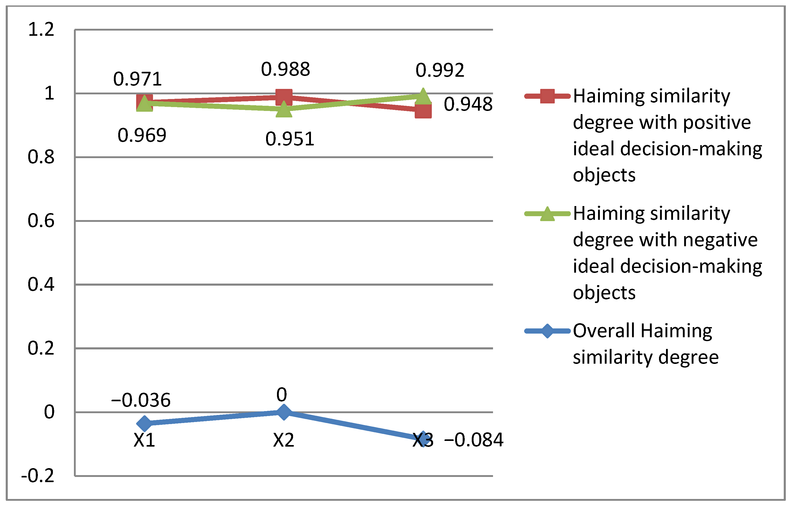
According to the results obtained in steps 5 and 6, it is easy to draw a geometric comparison diagram of Hamming similarity $S_{IN}^w\left(X_i,Z^{+\ast }\right)$ with a positive ideal decision object, Hamming similarity $S_{IN}^w\left(X_i,Z^{-\ast }\right)$ with a negative ideal decision object and overall Hamming similarity $OH{S}_{IN}\left(X_i\right)$, as shown in Figure 1. Although the three Hamming similarity values are not the same, the results of screening and ranking of the decision object set $\left\{X_i|i=1,2,3\right\}$ are consistent; all of them are $X_2\succ X_1\succ X_3$.

From Figure 1, it can be seen that the Hamming similarity degree curve with the positive ideal decision-making objects and the Hamming similarity degree curve with the negative ideal decision-making objects show opposite trends of change (this is due to the fact that the positive and negative ideal point series constitute different ideal decision objects), while the Hamming similarity degree curve with the positive ideal decision-making objects and the overall Hamming similarity degree curve show the same change trend. Moreover, the overall Hamming similarity degree curve appears steeper (this is caused by the aggregation of Hamming similarity degree information with positive ideal decision-making objects and Hamming similarity degree information with negative ideal decision-making objects), which can increase the decision-making discrimination.

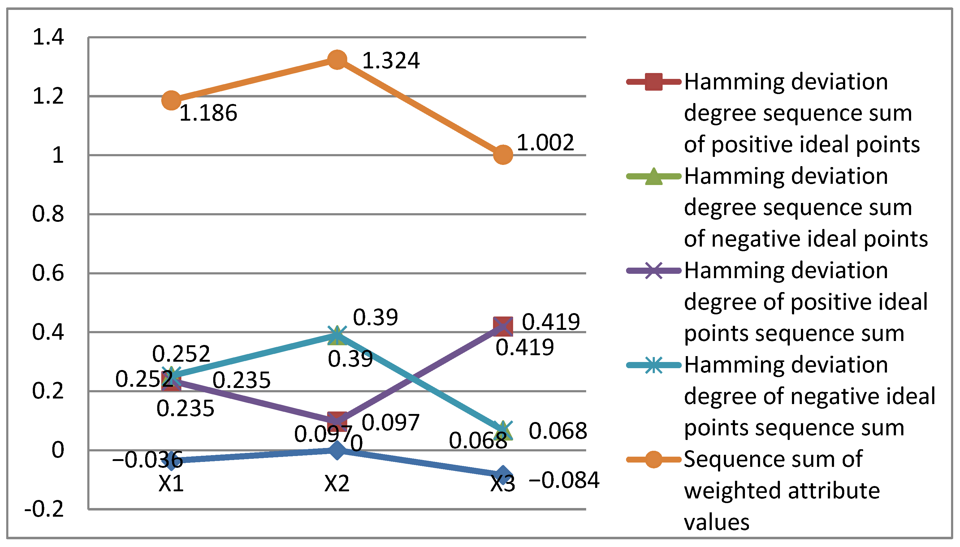
In addition to the above-mentioned screening and ranking of the alternative set by using the overall Hamming similarity superiority relation method for comparison among the decision-making objects, the conclusion of Theorem 3 in this paper can also be used, for example, to judge whether a decision object is good or bad by comparing its weighted attribute value with the Hamming distance sequence and size of the ideal point of the ideal decision object, or by comparing its weighted attribute value sequence and Hamming distance value of the ideal point sequence and the ideal point sequence of the ideal decision object, or by comparing the weighted attribute value sequence and size of the small element and the large element of the interval number of the optional decision object. We can easily obtain the following results by using Formula (9):

$$\begin{gathered} {\sum }_{j=1}^4{d}_{IN}\left({\tilde{x}}_{1u_j}^w,{\tilde{z}}_{u_j}^{+\ast }\right)=d_{IN}\left({\sum }_{j=1}^4{\tilde{x}}_{1u_j}^w,{\sum }_{j=1}^4{\tilde{z}}_{u_j}^{+\ast }\right)=0.235, \\ {\sum }_{j=1}^4{d}_{IN}\left({\tilde{x}}_{2u_j}^w,{\tilde{z}}_{u_j}^{+\ast }\right)=d_{IN}\left({\sum }_{j=1}^4{\tilde{x}}_{2u_j}^w,{\sum }_{j=1}^4{\tilde{z}}_{u_j}^{+\ast }\right)=0.097, \\ {\sum }_{j=1}^4{d}_{IN}\left({\tilde{x}}_{3u_j}^w,{\tilde{z}}_{u_j}^{+\ast }\right)=d_{IN}\left({\sum }_{j=1}^4{\tilde{x}}_{3u_j}^w,{\sum }_{j=1}^4{\tilde{z}}_{u_j}^{+\ast }\right)=0.419, \\ {\sum }_{j=1}^4{d}_{IN}\left({\tilde{x}}_{1u_j}^w,{\tilde{z}}_{u_j}^{-\ast }\right)=d_{IN}\left({\sum }_{j=1}^4{\tilde{x}}_{1u_j}^w,{\sum }_{j=1}^4{\tilde{z}}_{u_j}^{-\ast }\right)=0.252, \\ {\sum }_{j=1}^4{d}_{IN}\left({\tilde{x}}_{2u_j}^w,{\tilde{z}}_{u_j}^{-\ast }\right)=d_{IN}\left({\sum }_{j=1}^4{\tilde{x}}_{2u_j}^w,{\sum }_{j=1}^4{\tilde{z}}_{u_j}^{-\ast }\right)=0.390, \\ {\sum }_{j=1}^4{d}_{IN}\left({\tilde{x}}_{3u_j}^w,{\tilde{z}}_{u_j}^{-\ast }\right)=d_{IN}\left({\sum }_{j=1}^4{\tilde{x}}_{3u_j}^w,{\sum }_{j=1}^4{\tilde{z}}_{u_j}^{-\ast }\right)=0.068. \end{gathered}$$

or

$${\sum }_{j=1}^4\left(x_{1u_j}^{wL}+x_{1u_j}^{wU}\right)=1.186, {\sum }_{j=1}^4\left(x_{2u_j}^{wL}+x_{2u_j}^{wU}\right)=1.324, {\sum }_{j=1}^4\left(x_{3u_j}^{wL}+x_{3u_j}^{wU}\right)=1.002.$$

According to the above calculation results, it is easy to draw the geometric comparison diagram of Hamming distance sequence and ${\sum }_{j=1}^4{d}_{IN}({\tilde{x}}_{i{u}_j}^w,{\tilde{z}}_{u_j}^{+\ast })$ and ${\sum }_{j=1}^4{d}_{IN}({\tilde{x}}_{i{u}_j}^w,{\tilde{z}}_{u_j}^{-\ast })$ of the weighted attribute value of the decision object and the ideal point of the positive and negative ideal decision objects, Hamming distance sequence and $d_{IN}({\sum }_{j=1}^4{\tilde{x}}_{i{u}_j}^w,{\sum }_{j=1}^4{\tilde{z}}_{u_j}^{+\ast })$ and $d_{IN}({\sum }_{j=1}^4{\tilde{x}}_{i{u}_j}^w,{\sum }_{j=1}^4{\tilde{z}}_{u_j}^{-\ast })$ of the weighted attribute value sequence of the decision object and the ideal point sequence of the positive and negative ideal decision objects, weighted attribute value sequence and ${\sum }_{j=1}^4\left(x_{i{u}_j}^{wL}+x_{i{u}_j}^{wU}\right)$ of the interval number small element and large element of the decision object and the overall Hamming similarity $OH{S}_{IN}\left(X_i\right)$, as shown in Figure 2.

Although the Hamming deviation degree sequence sum of positive ideal points and Hamming deviation degree of positive ideal points sequence sum, Hamming deviation degree sequence sum of negative ideal points and Hamming deviation degree of negative ideal points sequence sum, sequence sum of weighted attribute values are not the same as the overall Hamming similarity value, the results of their screening and ranking of the decision object set $\left\{X_i|i=1,2,3\right\}$ are still consistent, both of which are $X_2\succ X_1\succ X_3$. From Figure 2, it can be seen that the Hamming degree of separation sequence and curve of positive and negative ideal points coincide with the Hamming degree of separation curve of positive and negative ideal point sequences, respectively (this is caused by the conclusion of Theorem 3 that the Hamming deviation degree sequence sum with ideal points of the ideal decision-making object and the Hamming deviation degree with ideal points sequence sum of the ideal decision-making object are equivalent). The Hamming degree of separation sequence and curve of positive ideal points, the Hamming degree of separation curve of positive ideal point sequence and the other four curves show the opposite change trend (this is because the selected target reference object is caused by the positive ideal decision object composed of the positive ideal point series), while the other four curves show the same change trend. Among them, the overall Hamming degree of similarity curve is compared with the weighted attribute value series and the sum of Hamming’s phase separation degree sequences of negative ideal points. The three curves of Hamming distance between the negative ideal point sequence and the negative ideal point sequence are more gentle (this is because the overall Hamming similarity curve integrates the Hamming similarity information of the weighted attribute value series and the positive and negative ideal point series, while the three curves of the weighted attribute value series and the Hamming distance between the negative ideal point sequence and the Hamming distance between the negative ideal point sequence and the negative ideal point sequence only fuse the small and large information of the interval number). Obviously, in the process of judging the advantages and disadvantages of the alternative decision-making objects, it can be judged by using the Hamming similarity between the alternative decision-making objects and the ideal optimal objects, which is reflected in the overall Hamming similarity $OH{S}_{IN}\left(X_i\right)$ in the whole object set, and the relevant conclusions of Theorem 3. This model is simple to implement and calculate and is easy to realize on the computer.

To facilitate comparative analysis, we use the multi-attribute decision-making algorithm weighted by the Interval Number-Based Decision-Making Object Maximizing Deviation Programming Model (IN-DMOMDPM) in [34,35] and the Interval Number-Based Decision-Making Object Probability Degree Relation Model (IN-DMOPDRM) in [27] to check the above cases, assuming that different physical dimension information among attribute measurement value data of the decision object has been unified; the attribute weight measurement formulas based on IN-DMOMDPM [34,35] and IN-DMOPDRM [27] algorithms are, respectively:

IN-DMOMDPM:

$$w_j=\frac{{\sum }_{i=1}^n{\sum }_{k=1}^n{d}_{IN}\left({\tilde{r}}_{ij},{\tilde{r}}_{kj}\right)}{{\sum }_{j=1}^m{\sum }_{i=1}^n{\sum }_{k=1}^n{d}_{IN}\left({\tilde{r}}_{ij},{\tilde{r}}_{kj}\right)},i\in N,j\in M.$$

(21)

IN-DMOPDRM:

$$w_j=\frac{{\sum }_{k=1,k\ne j}^m{\sum }_{i=1}^{n}p\left({\tilde{r}}_{ij}\ge {\tilde{r}}_{ik}\right)}{{\sum }_{j=1}^m{\sum }_{k=1,k\ne j}^m{\sum }_{i=1}^{n}p\left({\tilde{r}}_{ij}\ge {\tilde{r}}_{ik}\right)},i\in N,j,k\in M.$$

(22)

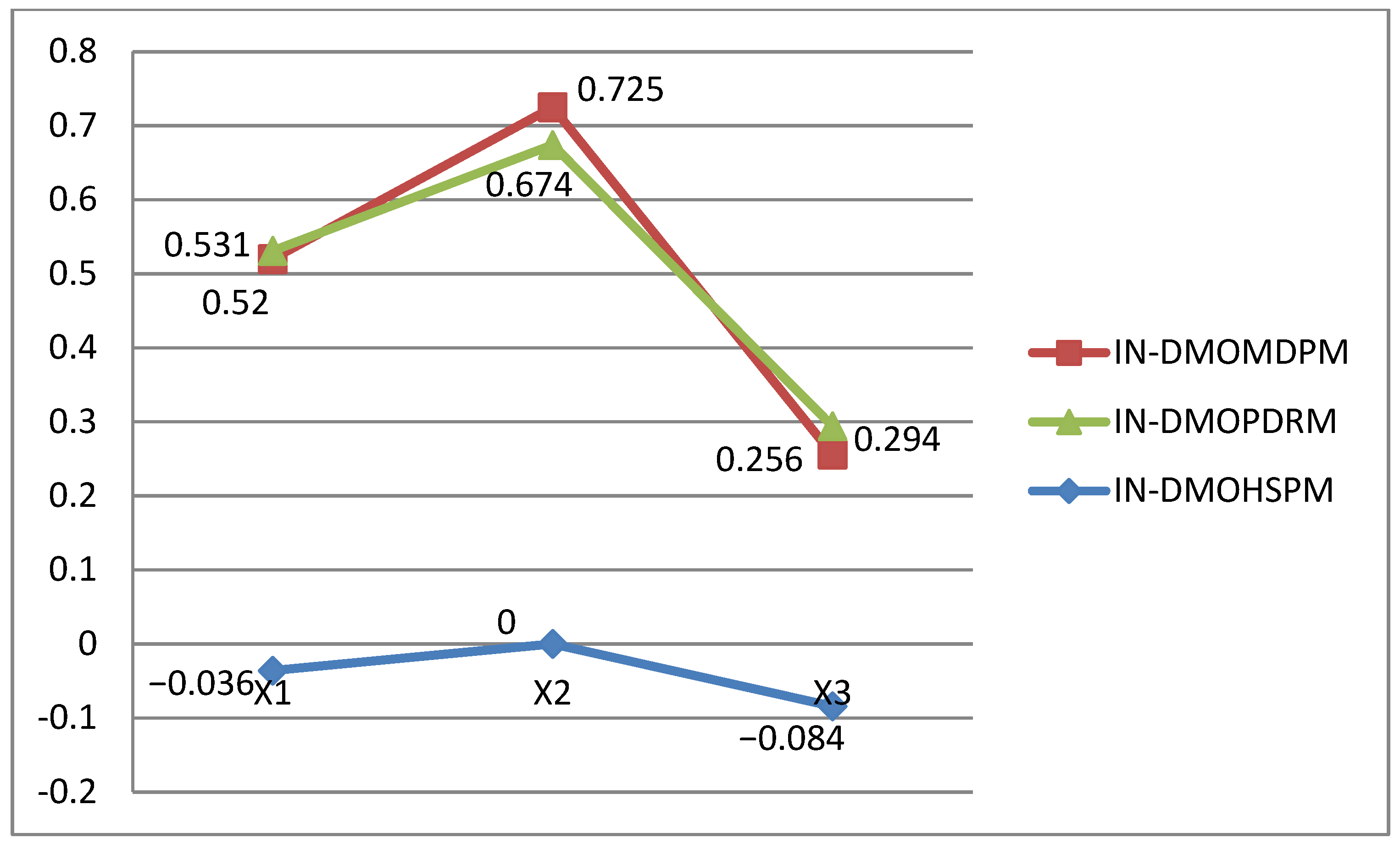
According to the implementation steps of the multi-attribute decision algorithm of IN-DMOMDPM and IN-DMOPDRM proposed in references [34,35] and [27] in dealing with the IN-UMADM problem, the above cases were checked and solved, and the following results were obtained:

IN-DMOMDPM:

$$X_2\underset{0.635}{\succ }{X}_1\underset{0.675}{\succ }{X}_3;$$

IN-DMOPDRM:

$$X_2\underset{0.593}{\succ }{X}_1\underset{0.656}{\succ }{X}_3.$$

Therefore, $X_2$ is the best supplier. The conclusion is consistent with the result of the IN-DMOHSPM algorithm. According to the above calculation results, there is no difficulty to draw the geometric comparison diagram of IN-DMOMDPM, IN-DMOPDRM and IN-DMOHSPM given in this paper, as shown in Figure 3.

It can be seen from Figure 3 that the three curves all show the same change trend, while the IN-DMOMDPM curve almost coincides with the IN-DMOPDRM curve, which is steeper than the IN-DMOHSPM gentle curve. Although it is convenient to increase the decision discrimination, it also increases the error of decision information in the process of aggregation. Although the three models and methods for determining the attribute weight measurement formula are different, the results of their screening and sequencing of the decision object set $\left\{X_i|i=1,2,3\right\}$ are consistent, and they are all $X_2\succ X_1\succ X_3$.

Through the comparative analysis of the above case of supplier selection, it is shown that the attribute weighting algorithm based on IN-DMOHSPM given in this paper is different from the attribute weighting algorithm based on IN-DMOMDPM given in the literature [34,35] and the attribute weighting algorithm based on IN-DMOPDRM given in the literature [27] in terms of weight measurement, but the three model algorithms are consistent in judging the advantages and disadvantages of the selection object set and screening and sorting, and can obtain the same optimal solution. Moreover, the attribute weighting algorithm based on IN-DMOHSPM proposed in this paper also integrates the similarity value information of attribute measure values. Compared with other existing methods, it can better reflect the similarity between the comprehensive attribute measure values of decision-making objects, which is more practical for the solution of the UMADM problem and convenient for data aggregation calculation and accurate fusion.

5. Conclusions

The attribute weight measurement based on the interval number-based decision-making object Hamming similar programming model (IN-DMOHSPM) is a new weighting idea proposed from the perspective of easy determination of the advantages and disadvantages of the selected objects and is also one of the important contents of UMADM problem research in this paper. The main idea is: after unifying the attribute measurement data with the different physical dimension information in the UMADM problem, the Hamming similarity degree value between the attribute measurement data of the decision-making object is too large, which indicates that the attribute plays a small role in the alternative decision making and should be given a small attribute weight value. Otherwise, the Hamming similarity degree value between the attribute measurement data of the decision-making object is too small, which indicates that the attribute plays an important role in the alternative decision making and should be given a large attribute weight value. In this paper, according to the attribute optimization and weighting thought based on IN-DMOHSPM and the comparative Hamming similarity superiority theory of interval numbers, the following three aspects are mainly studied for the UMADM problem where attribute weights are unknown with no preference for decision-making objects:

(1)

In order to investigate the degree of similarity of interval numbers, new definition formulas of Hamming similarity degree between normative interval numbers and Hamming similarity degree between decision-making objects are given, and the method of the single-objective optimization problem established by the interval number-based comparison Hamming similarity programming model is used to solve the optimal measurement formula of attribute weight.

(2)

Some relevant results of Hamming similarity superiority relation theory for interval numbers comparison are given, and it is deduced that the superiority between interval numbers, the comparison sizes of Hamming similarity degree value and the Hamming deviation degree value between interval numbers with the ideal point, as well as the sum sizes of small and large elements of attribute values of interval numbers, have been equivalent. However, the dominance among the selected alternative decision-making objects is equivalent to the comparison sizes of the Hamming similarity degree value of each selected decision-making object with the ideal optimal object, the Hamming deviation degree sequence sum sizes of the attribute value of the selected decision-making object with the ideal point value of the ideal optimal object, the Hamming deviation degree value of the attribute value sequence sum sizes of the selected decision-making object with the ideal point value sequence sum of the ideal decision-making object, and the attribute value sequence sum sizes of the interval number’s small element and large element of the selected decision-making object.

(3)

By using the overall Hamming similarity degree of each decision-making object compared with the ideal optimal object to screen and sort all of the selected alternative objects set, a new algorithm of the Hamming similarity programming model for interval number-based multiple attribute decision-making objects is presented.

In a word, there are some areas to be improved in the research work of this paper, and some deeper problem areas have not been touched. In terms of future research, two aspects needed to be further studied as follows: (1) How to carry out the research on consistency inspection, judgment and the consistency correction algorithm for interval number-based overall Hamming similarity degree function. How to build a single-objective programming optimization model containing a similar to comparative relative similarity degree between interval numbers, and extend various uncertain multi-attribute decision-making algorithms derived from the judgment of the merits on the selected decision-making objects to the UMADM problem, characterized by other types of fuzzy numbers (such as triangular fuzzy numbers, trapezoidal fuzzy numbers, intuitionistic fuzzy numbers, etc.), described and represented by other forms of judgment matrices (for example triangular fuzzy number judgment matrix, trapezoidal fuzzy number judgment matrix, intuitionistic fuzzy number judgment matrix, linguistic judgment matrix, etc.). (2) Due to the influence of objective factors, environmental restrictions and people’s subjective thinking judgment, people often encounter the situation that the utility value information of attribute measure is fuzzy, uncertain or imperfect (incomplete information), or even the utility value of attribute measure is represented by a mixture of interval numbers, triangular fuzzy numbers, trapezoidal fuzzy numbers, etc. How to aggregate and integrate the utility value information of attribute measure characterized by these different forms and how to construct a decision-making model and method to solve this kind of complex and mixed UMADM problem needs to be further explored.