Human Decision Time in Uncertain Binary Choice

Abstract

Decision time, also known as choice reaction time, has been frequently discussed in the field of psychology. The Hick–Hyman Law (HHL) has been a fundamental model that has revealed the quantitative relationship between the mean choice reaction time of human and the information entropy of stimuli. However, the HHL is only focused on rule-based behavior in which rules for selecting response according to stimulus are certain and neglects to model the knowledge-based behavior in which choices are uncertain and influenced by human belief. In this article, we explored the decision time related to one basic knowledge-based behavior—uncertain binary choice, where selections of response are determined by human belief degrees but not by stimuli uncertainties. Two experiments were conducted: one for verifying the HHL and the other for uncertain binary choice. The former (experiment) demonstrated the effectiveness of the HHL, and the latter one indicated that there is an exponential relationship existing between decision time and entropy of belief degree in uncertain binary choice. Moreover, data obtained from both experiments showed that the disturbance term of decision time should not be seen as probabilistic as existing studies have assumed, which highlighted the necessity and advantage of uncertain regression analysis.

1. Introduction

Decision time, also known as choice reaction time, is one of the important indexes used to characterize human performance [1]. In the 1950s, Hick [2] and Hyman [3] applied information theory to conduct several experiments and proposed a famous law called the Hick–Hyman Law (HHL). It demonstrated that the mean choice reaction time of humans would increase linearly as corresponding information entropy of stimuli raises. The inspiration for founding the HHL is intuitive, which is based on the fact that the more complex decisions always require longer time to initiate [1]. Consequently, the HHL has been widely accepted by the academic community and been used in fields involving assessment of human decision-making, such as psychology [4,5], neuroscience [6,7,8,9], and ergonomics [10,11]. Methods of improving and refining the HHL [4,5,12] have also been frequently discussed.

In a broad sense, researchers are used to dividing human behavior into three patterns: skill-based, rule-based, and knowledge-based [13]. Skill-based behavior refers to sensory-motor behavior achieved without using attention resources, rule-based behavior refers to procedural behavior using certain “If–then” rules pre-stored in the brain, and knowledge-based behavior refers to purposeful behavior that involves planning and reasoning. Essentially, the HHL and its improved versions are only effective in rule-based behavior [1] because, in this type of behavior, it has to be assumed that there are certain rules for selecting responses according to stimulus and they are well known to subjects (human) [14,15]. In other words, the HHL is not suitable for knowledge-based behavior in which choices are uncertain and influenced by human belief degrees.

Understanding how decision time performs in knowledge-based behavior is meaningful, because it can support us in predicting human performance time and further apply it to related fields, e.g., human reliability analysis [16], especially considering that knowledge-based behavior accounts for a large part of human behavior in practice. It is intuitive that the more uncertain (or complex) decisions always require a longer time to initiate in knowledge-based behavior. In this article, we mainly explored the decision time in a basic knowledge-based behavior—uncertain binary choice—and tried to reveal the quantitative relationship between decision time and difficulty of choice.

To do so, we newly designed an experiment with uncertain binary choice as its main content, in which subjects (human) needed to choose between two responses based on their belief degrees. Meanwhile, uncertainty theory [17] was used to express subjects’ belief degrees in the experiment, and correspondingly, the difficulty of choice was evaluated by the entropy [18] defined in the uncertainty theory. The reasons are clear: It has been demonstrated in several studies that, compared with other theories such as subjective probability [19], evidence theory [20], and possibility theory [21], uncertainty theory is more suitable for expressing human belief degree because it leads to a more robust, rigorous, and clear result that can significantly facilitate decision-making processes [22,23,24,25]. In addition, replacing the original guessing question of uncertain binary choice as its complementary question does not essentially change the difficulty of choice, which can be well reflected by the entropy in uncertainty theory that satisfies the property of symmetry. Along with the experiment of uncertain binary choice, we also conducted another experiment as a verification for HHL.

As a preview of the results, we found that the disturbance term of decision times obtained from two experiments could not be seen as white noise in the sense of probability. The existing studies on the HHL have rarely discussed this heteroscedasticity. Specifically, in Mordkoff’s work [4], as well as in the original work of Hick [2] and Hyman [3], the mean decision time was directly modeled without considering variations of data. Similarly, in the studies revealing the effects of factors that influence human decision time, such as response uncertainty [5], aging [8,26], misalignment [11], and cognitive control networks [12], the F-test or its extensions, e.g., analysis of variance (ANOVA), were widely used, which means that they directly assumed that the variation is a white noise in the sense of probability. In fact, researchers should handle this heteroscedasticity very carefully, because ignoring it may lead to biased conclusions, especially when working on prediction and comparison. Motivated by this, we used uncertain regression analysis [27], which is essentially not limited by the white-noise restriction mentioned above, instead of probabilistic regression tools in this article.

The remainder of the article is structured as follows. The preliminaries are presented in Section 2. Then, in Section 3, the procedures of the two experiments are clearly explained. Results and their analyses are shown in Section 4. Finally, related discussions are placed in Section 5, where we propose a conjecture on the general relationship between decision time and difficulty of choice in knowledge-based behavior.

2. Preliminaries

2.1. Hick–Hyman Law

In the 1950s, Hick and Hyman conducted several experiments and claimed that the mean choice reaction time ($RT$) of subjects (human) is a linear function of information entropy of stimuli. This finding, which is known as the Hick–Hyman Law, has already been a significant theory and been widely used in the fields of psychology, ergonomics, and human-machine systems. The central idea of the HHL can be described as:

$$RT=a+bH,$$

(1)

where $RT$ represents the mean choice reaction time of the subject, $a$ and $b$ represent the regression constants that can be estimated from experiment data, and $H$ (the units are bits) represents the information entropy of stimuli that is defined as follows:

$$H=-\sum p\left(i\right){\log }_2 p\left(i\right),$$

(2)

where $p\left(i\right)$ refers to the occurrence probability of one of the stimuli to which the subject can respond. In the case where the number of stimuli is $n$ and all probabilities of stimuli are equal, its corresponding information entropy can be calculated from:

$$H=-n·\frac{1}{n}{\log }_2 \frac{1}{n}={\log }_2 n.$$

(3)

2.2. Uncertainty Theory and Uncertain Regression Analysis

The uncertainty theory was developed by Liu [17] in 2007. In uncertainty theory, a concept of uncertain measure is used to model human belief degrees, which is defined as below:

Definition 1.

(Uncertain measure [17]). Let $\Gamma$ be a nonempty set, and $ℒ$ be $\sigma$-algebra over $\Gamma$. A set function is called an uncertain measure (represented by $ℳ$) if it satisfies the following axioms:

Axiom 1.

(Normality Axiom). $ℳ\left\{\Gamma \right\}=1$ for the universal set $\Gamma$.

Axiom 2.

(Duality Axiom). $ℳ\left\{\Lambda \right\}+ℳ\left\{{\Lambda }^c\right\}=1$ for any event $\Lambda \in ℒ$.

Axiom 3.

(Subadditivity Axiom). For every countable sequence of event ${\Lambda }_1,{\Lambda }_2,\cdots$, we have:

$$ℳ\left\{{\displaystyle \underset{i=1}{\overset{\infty }{\cup }}}{\Lambda }_i\right\}\le {\displaystyle \sum _{i=1}^{\infty }}ℳ\left\{{\Lambda }_i\right\}.$$

(4)

The triplet $\left(\Gamma ,ℒ,ℳ\right)$ is called an uncertainty space. The product uncertain measure was proposed by Liu [18] in 2009, and thus the fourth axiom of uncertainty theory was produced.

Axiom 4.

(Product Axiom). Let $\left({\Gamma }_k,{ℒ}_k,{{\rm M}}_k\right)$ be uncertainty spaces for $k=1,2,\cdots$ The product uncertain measure, $ℳ$, is an uncertain measure satisfying:

$$ℳ\left\{{\displaystyle \prod _{k=1}^{\infty }}{\Lambda }_k\right\}={\displaystyle \underset{k=1}{\overset{\infty }{\wedge }}}{{\rm M}}_k\left\{{\Lambda }_k\right\},$$

(5)

where ${\Lambda }_k$ are arbitrarily chosen events from ${ℒ}_k$ for $k=1,2,\cdots$, respectively.

Definition 2.

(Uncertain variable [17]). An uncertain variable is a function, $\xi$, from an uncertainty space $\left(\Gamma ,ℒ,ℳ\right)$ to the set of real numbers such that $\left\{\xi \in B\right\}$ is an event for any Borel set, $B,$ of real numbers.

Definition 3.

(Uncertainty distribution [17]). The uncertainty distribution, $\Phi$, of an uncertain variable, $\xi$, is defined by:

$$\Phi \left(x\right)=ℳ\left\{\xi \le x\right\}$$

(6)

for any real number $x$.

Example 1.

Take an uncertainty space $\left(\Gamma ,ℒ,ℳ\right)$ to be $\left({\gamma }_1,{\gamma }_2\right)$ with power set and $ℳ\left\{{\gamma }_1\right\}=0.8$, $ℳ\left\{{\gamma }_2\right\}=0.2$. Then, the uncertain variable

$$\xi \left(\gamma \right)=\{\begin{array}{cc}0,& \mathrm{if} \gamma ={\gamma }_1\\ 1,& \mathrm{if} \gamma ={\gamma }_2\end{array}$$

(7)

has an uncertainty distribution:

$$\Phi \left(x\right)=\{\begin{array}{cc}0,& if x<0\\ 0.8,& if 0\le x<1\\ 1,& if x\ge 1.\end{array}$$

(8)

Definition 4.

(Normal uncertainty distribution [28]) An uncertain variable, $\xi$, is called normal if it has a normal uncertainty distribution

$$\Phi \left(x\right)={\left(1+exp\left(\frac{\pi \left(e-x\right)}{\sqrt{3}\sigma }\right)\right)}^{-1}, x\in \Re ,$$

(9)

denoted by $\mathcal{N}\left(e,\sigma \right)$, where $e$ and $\sigma$ are real numbers with $\sigma >0$. A normal uncertainty distribution is called standard if $e=0$ and $\sigma =1$.

Definition 5.

(Regular uncertainty distribution [28]) An uncertainty distribution, $\Phi \left(x\right)$, is said to be regular if it is a continuous and strictly increasing function with respect to $x$ at which $0<\Phi \left(x\right)<1$, and

$$\underset{x\to -\infty }{lim}\Phi \left(x\right)=0,\underset{x\to +\infty }{lim}\Phi \left(x\right)=1.$$

(10)

Definition 6.

(Inverse uncertainty distribution [28]) Let $\xi$ be an uncertain variable with regular uncertainty distribution, $\Phi \left(x\right)$. Then the inverse function, ${\Phi }^{-1}\left(\alpha \right)$, is called the inverse uncertainty distribution of $\xi$.

Example 2.

The inverse uncertainty distribution of normal uncertain variable, $\mathcal{N}\left(e,\sigma \right)$, is

$${\Phi }^{-1}\left(\alpha \right)=e+\frac{\sigma \sqrt{3}}{\pi }ln\frac{\alpha }{1-\alpha }$$

(11)

Definition 7.

(Expected value [17]) Let $\xi$ be an uncertain variable. Then the expected value of $\xi$ is defined by

$$E\left[\xi \right]={\int }_0^{+\infty }ℳ\left\{\xi \ge x\right\}dx-{\int }_{-\infty }^0ℳ\left\{\xi \le x\right\}dx$$

(12)

provided that at least one of the two integral is finite.

Definition 8.

(Variance [17]) Let $\xi$ be an uncertain variable with finite expected value, $e$. Then the variance of $\xi$ is

$$V\left[\xi \right]=E\left[{\left(\xi -e\right)}^2\right].$$

(13)

Example 3.

A normal uncertain variable, $\xi \sim \mathcal{N}\left(e,\sigma \right)$, has an expected value, $e$, and a variance, ${\sigma }^2$.

Definition 9.

(Entropy [18]) Suppose that $\xi$ is an uncertain variable with uncertainty distribution, $\Phi$. Then its entropy is defined by

$$H\left[\xi \right]={\int }_{-\infty }^{+\infty }S\left(\Phi \left(x\right)\right)dx$$

(14)

where $S\left(t\right)=-t ln t-\left(1-t\right) ln\left(1-t\right)$.

Example 4.

Let $\xi$ be the uncertain variable defined in Example 1. It then follows from the definition of entropy that

$$\begin{array}{cc}\hfill H\left[\xi \left(\gamma \right)\right]=& -{\int }_{-\infty }^0\left(0 ln 0+1 ln 1\right)dx\hfill \\ & -{\int }_0^1\left(0.8 ln 0.8+0.2 ln 0.2\right)dx\hfill \\ & -{\int }_1^{+\infty }\left(1 ln 1+0 ln 0\right)dx\hfill \\ \hfill =& 0.5004.\hfill \end{array}$$

Uncertain regression analysis was developed to discover the relationship between explanatory variables and response variables [27]. Mathematically, the functional relationship between the explanatory variables $\left(x_1,x_2,\cdots ,x_p\right)$ and the response variable, $y$, is expressed by an uncertain regression model:

$$y=f\left(x_1,x_2,\cdots ,x_p|\beta \right)+\epsilon ,$$

(15)

where $\beta$ is a vector of parameters, and $\epsilon$ is an uncertain disturbance term, i.e., an uncertain variable [29]. After defining the uncertain regression model, several steps can be conducted to analyze the relationship between explanatory variables and response variables.

Step 1. Parameter estimation [27]. Assume a set of observed data, $\left(x_{i1},x_{i2},\cdots ,x_{ip},y_i\right)$, $i=1,2,\cdots ,n$, is obtained. The least squares estimate of $\beta$ in the uncertain regression model is the solution, $\widehat{\beta }$, of the minimization problem:

$$\underset{\beta }{\min }\sum _{i=1}^n{\left(y_i-f\left(x_{i1},x_{i2},\cdots ,x_{ip}|\beta \right)\right)}^2.$$

(16)

Thus, the fitted regression model is

$$f(x_1,x_2,\cdots ,x_p|\widehat{\beta }).$$

(17)

Definition 10.

(Residual [30]) Let $\left(x_{i1},x_{i2},\cdots ,x_{\mathrm{ip}},y_i\right)$, $i=1,2,\cdots ,n$ be a set of observed data, and let Equation (17) represents the fitted regression model. Then, for each index, $i$ $\left(i=1, 2,\cdots ,n\right)$, the term

$${\epsilon }_i=y_i-f(x_{i1},x_{i2},\cdots ,x_{\mathrm{ip}}|\widehat{\beta })$$

(18)

is called the $i$-th residual.

Step 2. Residual analysis [30]. The residuals ${\epsilon }_1,{\epsilon }_2,\cdots ,{\epsilon }_n$ calculated from Equation (18) are regarded as the samples of the uncertain disturbance term, $\epsilon$, in the uncertain regression model. The expected value of $\epsilon$ can be estimated as the average of residuals, i.e.,:

$$\widehat{e}=\frac{1}{n}\sum _{i=1}^n{\epsilon }_i$$

(19)

And the variance can be estimated as

$${\widehat{\sigma }}^2=\frac{1}{n}\sum _{i=1}^n{\left({\epsilon }_i-\widehat{e}\right)}^2.$$

(20)

Therefore, the estimated disturbance term, $\widehat{\epsilon }$, is an uncertain variable with expected value, $\widehat{e}$, and variance, ${\widehat{\sigma }}^2$.

Step 3. Uncertain hypothesis test [31]. If we further assume that $\widehat{\epsilon }$ follows the normal uncertainty distribution, $\mathcal{N}(\widehat{e},\widehat{\sigma })$, then we will obtain an uncertain regression model:

$$y=f(x_1,x_2,\cdots ,x_p|\widehat{\beta })+\mathcal{N}(\widehat{e},\widehat{\sigma }).$$

(21)

After this, the uncertain hypothesis test can be used to see if the uncertain regression model fits the observed data well. Two hypotheses should be established:

$$H_0:e=\widehat{e} \mathrm{and} \sigma =\widehat{\sigma } \mathrm{vs}. H_1:e\ne \widehat{e} \mathrm{or} \sigma \ne \widehat{\sigma },$$

where $e$ and ${\sigma }^2$ represent the mean and variance of uncertain disturbance term $\epsilon$, respectively. Given a significance level of $\alpha$ (e.g., 0.05), the test for the hypotheses can be developed, which is:

$$\begin{array}{r}W=\{\left(z_1,z_2,\cdots ,z_n\right):\mathrm{there} \mathrm{are} \mathrm{at} \mathrm{least} \alpha \mathrm{of} \mathrm{indexes} i’\mathrm{s} \mathrm{with} 1\le i\\ \le n \mathrm{such} \mathrm{that} z_i<{\Phi }^{-1}\left(\frac{\alpha }{2}\right) \mathrm{or} z_i>{\Phi }^{-1}\left(1-\frac{\alpha }{2}\right)\},\end{array}$$

where ${\Phi }^{-1}$ is the inverse uncertainty distribution of $\mathcal{N}\left(\widehat{e},\widehat{\sigma }\right)$, i.e.,:

$${\Phi }^{-1}\left(\alpha \right)=\widehat{e}+\frac{\widehat{\sigma }\sqrt{3}}{\pi }ln\frac{\alpha }{1-\alpha }.$$

(22)

For the $n$ determined residuals, ${\epsilon }_1,{\epsilon }_2,\cdots ,{\epsilon }_n$, if $\left({\epsilon }_1,{\epsilon }_2,\cdots ,{\epsilon }_n\right)\in W,$ then we reject $H_0$. If $\left({\epsilon }_1,{\epsilon }_2,\cdots ,{\epsilon }_n\right)\notin W,$ then we accept $H_0$. In this case, it can be concluded that the uncertain regression model expressed as Equation (21) is a good fit to the observed data.

3. Methods

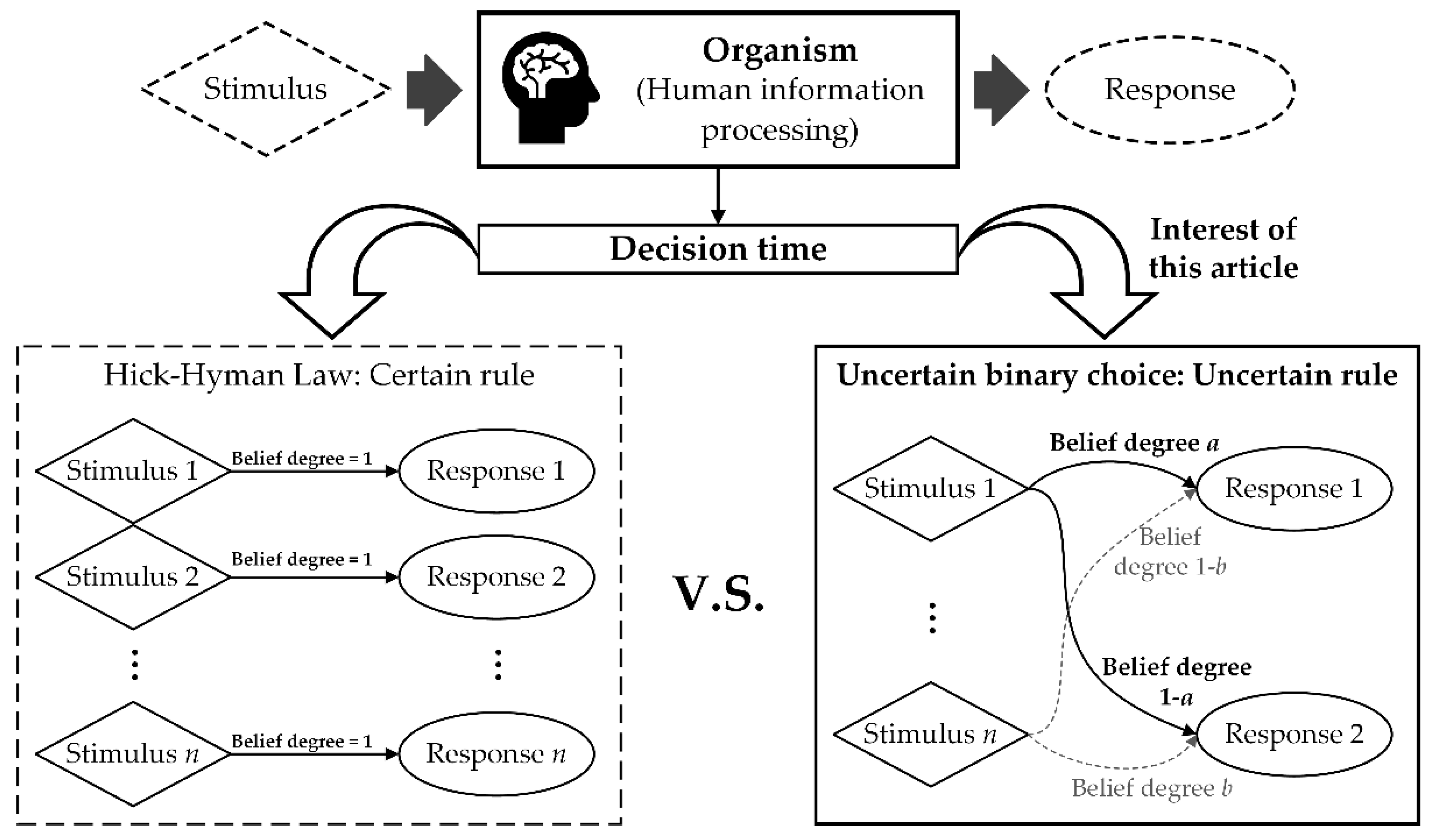
The stimulus-Organism-Response (S-O-R) paradigm [32] is a basic explanation of human behavior mechanisms in psychology. The “O” part, which happens between stimulus and response, is commonly seen as human information processing, which essentially represents the process of human cognition; see Figure 1. Human information processing is a process that shows different patterns in different circumstances. In Reason’s SRK framework [33], human information processing is classified into three kinds of pattern: skill-based, rule-based, and knowledge-based. The skill-based pattern appears in particularly familiar tasks for human, during which the control of human behavior is entrusted to a pre-stored action sequence mode, so that the subject needs no attention resources in this pattern. The rule-based pattern dominates when the subject is performing routine tasks that require the subject to consciously use the “If–then” rules stored in the brain with a certain amount of attention. Finally, the knowledge-based pattern happens in unfamiliar or unexpected situations for the subject. In this pattern, the subject must consume great attention resources on the current task to decide the best response. Reasoning is seen as a typical knowledge-based pattern.

The HHL, essentially, is proposed for revealing the characteristics of choice reaction time related to rule-based behavior pattern [1]. Conventionally, in experiments related to the HHL, it is assumed that the occurrences of stimuli are random. But the right choice response that should be made according to each stimulus is certain and is well known to subjects, i.e., there are certain “If–then” rules and they are clear to the subjects. This property is expressed by the mark “Belief degree = 1” in the lower left of Figure 1. Through this setting, a high degree of compatibility is established between stimuli and responses, and thus the entropy of stimuli is inherited to the entropy of human responses without introducing any extra bias [5]. As a result, a connection is achieved between an objective index—information entropy of stimuli—and a basic property of human behavior—choice reaction time.

However, such connections break in knowledge-based behavior. In the knowledge-based pattern, there are no certain choice rules between stimuli and responses, and a subject’s choice as a response to any stimulus is totally determined from his/her belief degree. To explore how this belief degree affects human decision time in knowledge-based behavior, we designed an experiment called uncertain binary choice. The basic idea of uncertain binary choice is shown in the lower right of Figure 1. In every round of this experiment, one stimulus would be displayed, which can be regarded as a clue regarding a truth, and what subjects needed to do was to choose between two responses, as a guess at the truth. Obviously, the choice was based on the subject’s belief degree. We used the uncertain measure to represent this belief degree and tried to understand the relationship between the decision time and difficulty of choice, in which the difficulty was evaluated by the entropy of uncertain measure. The detailed explanation of the uncertain binary choice experiment is shown in Section 3.2. Before this, another experiment that was the same as conventional HHL experiments had been conducted. The procedures of these two experiments are explained in the following.

3.1. Experiment 1: Hick–Hyman Law

The aim of Experiment 1 was to demonstrate the HHL. To do so, we developed an experimental computer program based on Psychtoolbox-3 [34]. The detailed description of this experiment is shown as follows.

3.1.1. Apparatus and Participants

The apparatus of Experiment 1 consisted of a computer, a 24-inch visual display (screen), and a mouse. The experimental program, whose function was to present stimuli on the visual display and to record the subjects’ choice reaction times, had been pre-installed on the computer before the experiment. Subjects’ selections as responses to stimuli were achieved by clicking the mouse; the rules of selection will be explained in the next section. Three participants (subjects), all around the age of 28, were involved in the experiment. All of them were postgraduates at Beihang University and volunteered in this experiment. Similar to the works of Hick [2], Hyman [3], and Wifall [5], the purpose of this paper is to reveal the basic characteristics of decision time, in which intervention and comparison are not involved. Therefore, we believed that the number of participants would not significantly change the characteristics of the data. Meanwhile, the fact that the data of the three subjects had the same characteristics has also supported this point.

3.1.2. Procedure

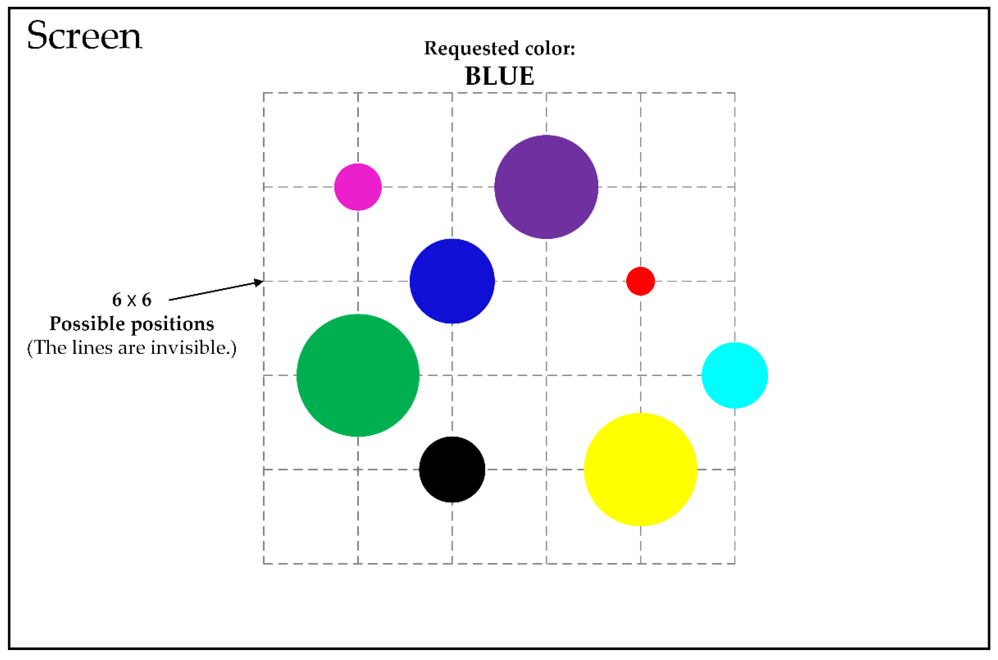
Each trial began with the presentation of circles (stimuli) with different colors and sizes on the screen; see Figure 2. Here, the possible colors of circles included black, red, green, blue, pink, light green, yellow, and purple. In each trial, the number of circles was an integer randomly generated from numbers between 1 and 8. In addition, the sizes of the circles were randomly determined, and the generated circles were randomly arranged at positions in the intersection of 6 rows and 6 columns (rows and columns are invisible) settled in the middle of the screen. The purposes of such arrangement were (a) to avoid any obvious grouping of circles, (b) to obviate the subjects’ learning of the positions of circles, and (c) to avoid any needs for apparent eye movements that may increase choice reaction times.

In each trial, the color of one of the generated circles was randomly selected as a request that would be presented at the top of screen, as shown in Figure 2, and what subjects needed to do was to click the mouse on the target circle corresponding to the requested color as a response. Participants were instructed to respond as quickly and accurately as possible. Each subject participated in 30 trials at a time, followed by a ten-minutes break. Three subjects participated in a total of 300 trials, in which one of them did 120 trials and the other two did 90 trials, respectively.

Because the probabilities of occurrence of stimuli (circles with different colors) are equal in each trial, we used Equation (3) presented in Section 2.1 to evaluate the entropy of stimuli. For example, if 4 circles of different colors appeared in a trial, then the entropy of stimuli in this trial would be 2 bits. Furthermore, the time interval between the beginning of a trial and the subject’s corresponding response was recorded as a choice reaction time. As a result, a total of 300 different combinations of stimulus entropy and choice reaction time were collected at the end of Experiment 1.

3.2. Experiment 2: Uncertain Binary Choice

We designed Experiment 2 for the purpose of exploring the relationship between decision time and entropy of human belief degree under uncertain binary choice. We developed an experimental computer program based on Psychtoolbox-3 [34] to conduct this experiment. Descriptions of Experiment 2 are presented as follows.

3.2.1. Apparatus and Participants

The apparatus of Experiment 2 was the same as that of Experiment 1, i.e., it included a computer, a 24-inch visual display (screen), and a mouse. The experimental program had been pre-installed on the computer and its function was to present stimuli on the screen and to record subjects’ decision times. Subjects’ selections as responses to stimuli were also achieved by clicking the mouse. The three participants in Experiment 1 were selected as the subjects in Experiment 2.

3.2.2. Procedure

The basic idea of uncertain binary choice experiment was that: One stimulus would be displayed as a clue about a truth in each trial, and what subjects needed to do was to choose one between two responses as a guess at the truth, where the subjects’ choices were based on their belief degrees. We used uncertain measure to express the subjects’ belief degrees and tried to find how the difficulty of choice affects decision time, in which the difficulty of choice was evaluated by the entropy of uncertain measure.

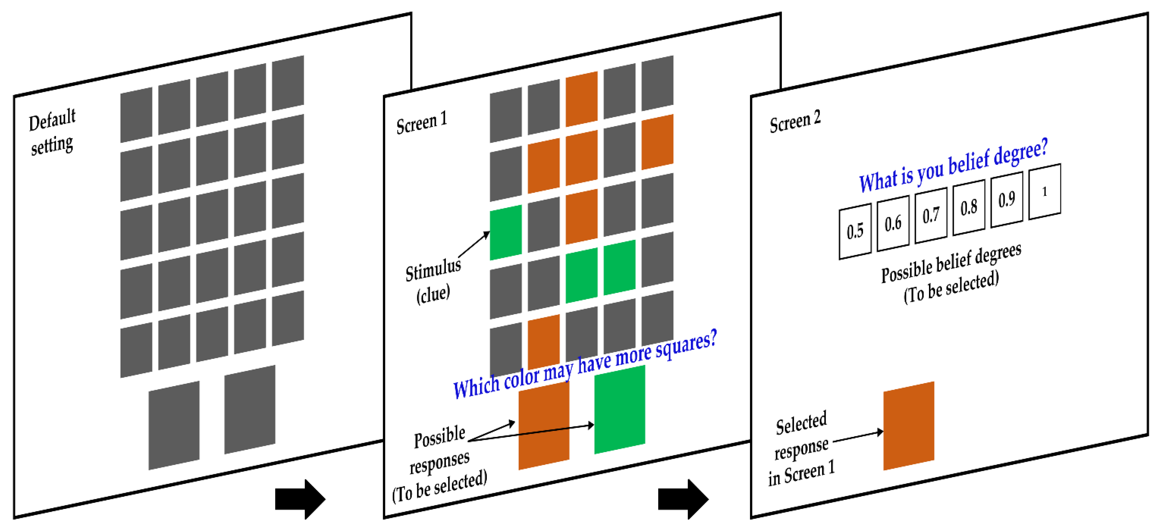
The guessing process of our experiment is shown in Figure 3. Before the trial, 25 squares were placed in 5 rows and 5 columns at the middle of the screen, of which the reverse sides (in grey) were facing to subjects. Meanwhile, the obverse side (invisible to the subjects) of each of these squares was painted in one of two optional colors at random. It should be noted that the two optional colors were also determined randomly for each trial, i.e., they were not the same in different trials. Because the subjects could only see the reverse sides of squares, they were unaware of information regarding the assignment of colors in the obverse sides of these squares, as well as which color had more squares. These constituted the default setting of a trial. Here is a simple example to improve understanding: If in a random assignment of a trial, orange and green are selected as the optional colors and obverse sides of 9 of the 25 squares happened to be painted in orange, then the obverse sides of the remaining 16 squares will be in green (but this information is unknown to the subjects). When the trial began, as shown in Screen 1 in Figure 3, the program randomly selected a number (1 to 25) of squares to flip, which led to obverse sides of the flipped squares faceing the subjects so that the subjects would be aware of the determined colors of these flipped squares. This was regarded as the stimulus in each trial. After the display of stimulus, the subjects were asked the question—“Which color might have more squares in all of 25 squares?”—and were required to show their selection by clicking on one of two big colored squares presented at the bottom of screen. Because the number of possible responses was two, we called this experiment as uncertain binary choice. We defined the decision time as the time interval between the beginning of the trial and the time point when a subject selected a response in Screen 1. After subjects had made a choice, the program turned to the next part, i.e., Screen 2 in Figure 3, where the subjects were asked to show their belief degree on the choice already made. This was done by choosing one of six numbers ranging from 0.5 to 1.

In each trial, the two selectable options for the subject were described by an uncertain variable, $\xi$, where $\xi =0$ represented the subject’s selection being made and $\xi =1$ represented the other, i.e.,:

$$\xi =\{\begin{array}{cc}0,& \text{subject}’\mathrm{s} \mathrm{selection},\\ 1,& \mathrm{the} \mathrm{other}.\end{array}$$

(23)

If $j$ represent the value of the subject’s belief degree chosen on Screen 2 in Figure 3, the uncertainty distribution of $\xi$ would be:

$$\Phi \left(x\right)=\{\begin{array}{cc}0,& \mathrm{if} x<0\\ j,& \mathrm{if} 0\le x<1,\\ 1,& \mathrm{if} x\ge 1.\end{array}$$

(24)

where $j=0.5, 0.6,\cdots , 1$. Correspondingly, the entropy of the subject’s belief degree can be determined from Equation (14). The relationship between belief degree and entropy obtained from this step is shown in

Table 1. The relationship between belief degree and entropy.

Belief Degree j	0.5	0.6	0.7	0.8	0.9	1
Entropy	0.6931	0.6730	0.6109	0.5004	0.3251	0

. It should be noted that, in this experiment, if we change the question to “which color might have fewer squares?”, the difficulty of choice will not change in essence. Fortunately, such change does not affect the value of entropy shown in Table 1 as well, because the $S\left(t\right)$ involved in Equation (14) strictly satisfies the property of symmetry, which highlights that the definition of entropy in uncertainty theory is quite reasonable.

The subjects were instructed to respond as earnestly as possible. Similar to Experiment 1, each subject participated in 30 trials at a time, followed by a ten-minutes break. Three subjects participated in a total of 300 trials, in which one of them did 120 trials and the other two did 90 trials, respectively. As a result, a total of 300 different combinations of entropy and decision time were collected at the end of Experiment 2.

4. Results

4.1. Experiment 1

The observed data of Experiment 1 consisted of 300 combinations of stimuli entropy and choice reaction time, which can be represented as

$$\left(x_i^{\left(1\right)},y_i^{\left(1\right)}\right), i=1, 2,\cdots 300,$$

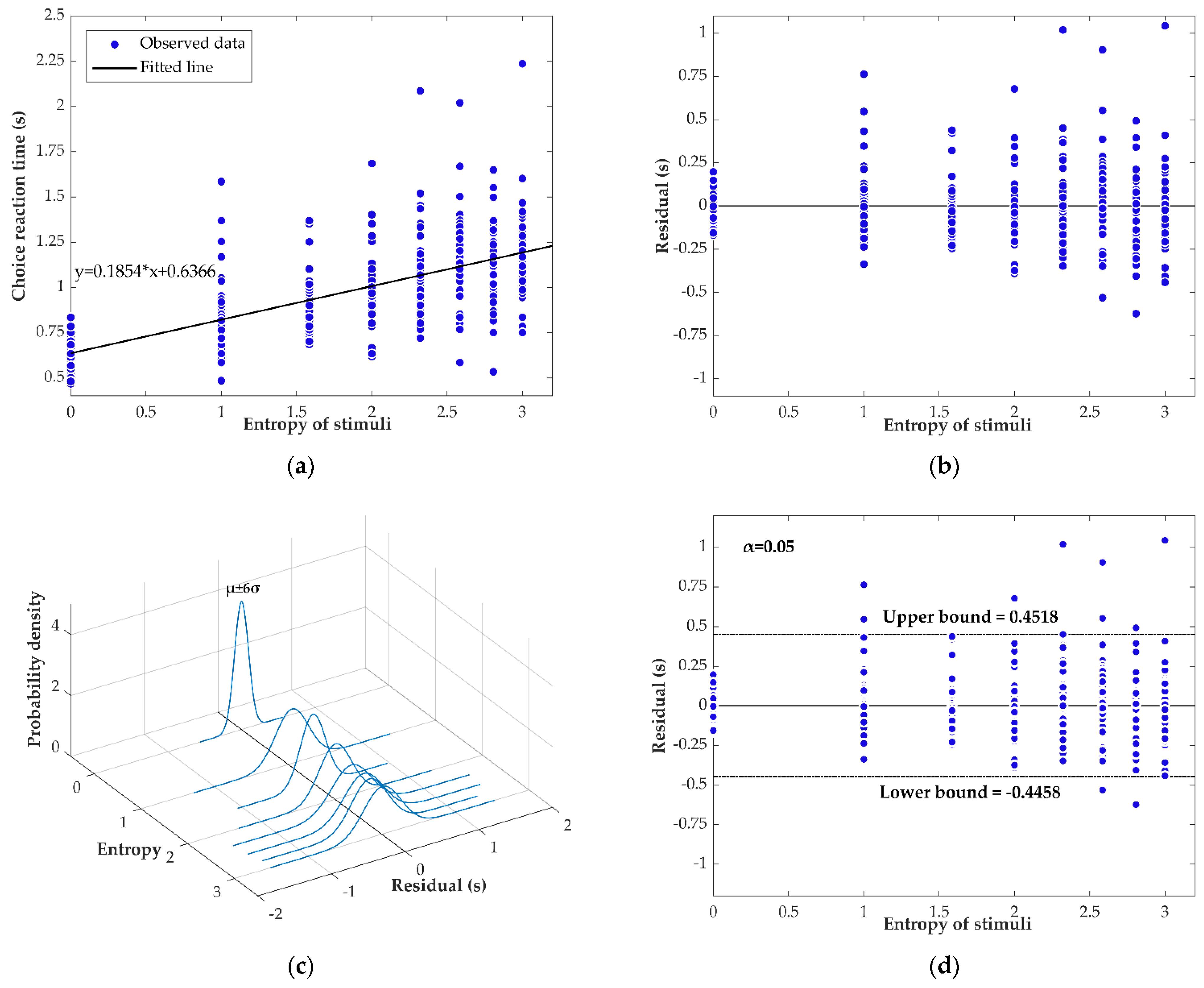
where $x_i^{\left(1\right)}$ and $y_i^{\left(1\right)}$ represent stimuli entropy and choice reaction time in the $i$-th trial, respectively. The amount of data corresponding to different numbers of stimuli are shown in

Table 2. Number of data in each case.

Numbers of Stimuli	One	Two	Three	Four	Five	Six	Seven	Eight
Entropy	0	1	1.5850	2	2.3219	2.5850	2.8074	3
Amount of data	40	38	36	38	36	38	34	40

. The observed data are plotted in Figure 4a.

According to Equation (16), we used the linear equation

$$y=\beta ·x+\theta$$

(25)

to fit the data and eventually determine the fitted regression model, i.e., the best fitting line:

$$y^{\left(1\right)}=0.1854·x^{\left(1\right)}+0.6366,$$

(26)

where $x^{\left(1\right)}$ refers to information entropy of stimuli and $y^{\left(1\right)}$ refers to choice reaction time.

It should be noted that the value of parameter $\theta$ in Equation (25) was set to be equal to the mean—0.6366—of choice reaction times of the case in which the number of stimuli is one. The reason for this is that, in the HHL, the constant is regarded as the sum of those processing latencies that are unrelated to the reduction of uncertainty [1], e.g., the time spent on encoding the stimulus and executing the response, and this should be the mean choice reaction time in the case in which only one stimulus occurs.

According to Equation (18), we calculated the residuals of data $({\epsilon }_1^{(1)},{\epsilon }_2^{(1)},\cdots ,{\epsilon }_{300}^{(1)})$, and plotted them in Figure 4b. It can be clearly seen from the figure that there is obvious heteroscedasticity existing in the residuals plot. To make it clearer, we plotted the normal probability density distributions of these residuals regarding different entropy in Figure 4c, ranging from six standard deviations below the mean to six standard deviations above the mean, and these distributions clearly showed that the disturbance term of these data could not be seen as white noise in the sense of probability. Therefore, we concluded that probability-based regression tools were not suitable for analyzing the disturbance term of these data.

Considering this, we regarded the disturbance term as an uncertain variable, ${\epsilon }^{(1)}$, whose samples are $({\epsilon }_1^{(1)},{\epsilon }_2^{(1)},\cdots ,{\epsilon }_{300}^{(1)})$. By using Equations (19) and (20), we assumed that the estimated disturbance term, ${\widehat{\epsilon }}^{\left(1\right)}$, follows uncertainty distribution $\mathcal{N}\left(0.0030,0.2222\right)$. That is to say, the estimated relationship between choice reaction time and information entropy of the stimuli, i.e., the uncertain regression model in Experiment 1 could be represented as:

$$y^{\left(1\right)}=0.1854·x^{\left(1\right)}+0.6366+\mathcal{N}\left(0.0030,0.2222\right).$$

(27)

Then, we used the uncertain hypothesis test to see if the uncertain regression model fitted the observed data well. Correspondingly, two hypotheses were established:

$$H_0:e^{\left(1\right)}=0.0030 \mathrm{and} {\sigma }^{\left(1\right)}=0.2222 \mathrm{versus} H_1:e^{\left(1\right)}\ne 0.0030 \mathrm{or} {\sigma }^{\left(1\right)}\ne 0.2222,$$

where $e^{\left(1\right)}$ and ${\sigma }^{\left(1\right)}$ represent, respectively, the mean and standard deviation of the uncertain disturbance term, ${\epsilon }^{\left(1\right)}$. Given a significance level $\alpha =0.05$, a test for the hypotheses was developed, which was:

$$W^{\left(1\right)}=\left\{\left(z_1,z_2,\cdots ,z_{300}\right):\mathrm{there} \mathrm{are} \mathrm{at} \mathrm{least} 15 \mathrm{of} \mathrm{indexes} i’\mathrm{s} \mathrm{with} 1\le i\le 300 \mathrm{such} \mathrm{that} z_i<-0.4458 \mathrm{or} z_i>0.4518\right\}.$$

Because only 11 of the choice reaction times were involved in $W^{\left(1\right)}$ (See Figure 4d), we have $\left({\epsilon }_1^{\left(1\right)},{\epsilon }_2^{\left(1\right)},\cdots ,{\epsilon }_{300}^{\left(1\right)}\right)\notin W^{\left(1\right)}$. Thus, the uncertain regression model (27) can be seen as a good fit to the observed data, which demonstrates that the linear relationship claimed in the HHL is effective.

4.2. Experiment 2

The observed data of Experiment 2 consisted of 300 combinations of entropy of belief degree and decision time, which can be expressed as:

$$\left(x_i^{\left(2\right)},y_i^{\left(2\right)}\right), i=1,2,\cdots 300,$$

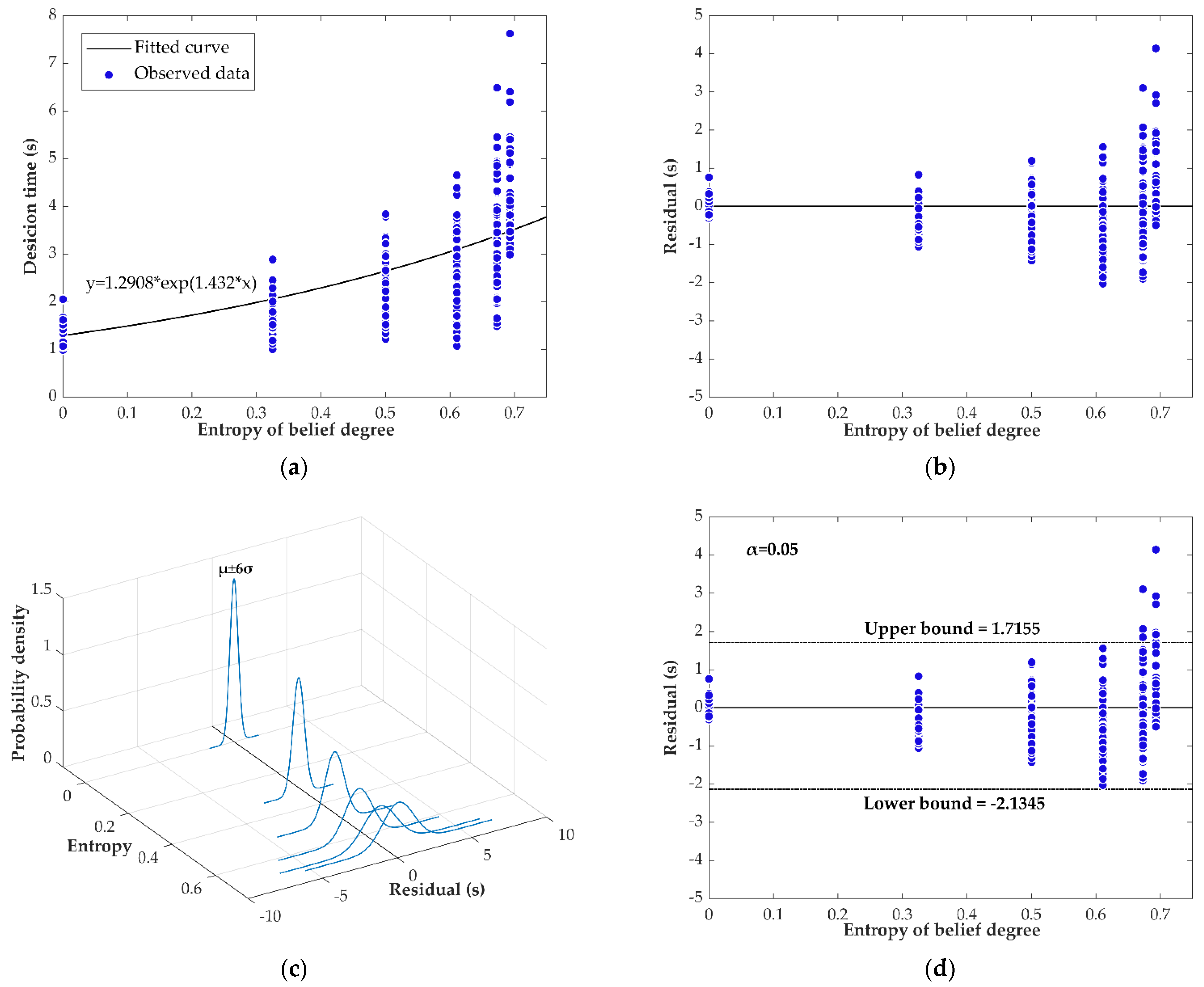
where $x_i^{\left(2\right)}$ and $y_i^{\left(2\right)}$ represent entropy of belief degree and decision time in the $i$-th trial, respectively. Amount of data corresponding to different belief degree are shown in

Table 3. Amount of data in each case.

Belief Degree $\mathit{j}$	0.5	0.6	0.7	0.8	0.9	1
Entropy $E^{\left(j\right)}$	0.6931	0.6730	0.6109	0.5004	0.3251	0
Amount of data $N^{\left(j\right)}$	40	57	63	76	44	20

. The observed data are plotted in Figure 5a.

We used

$$y=f\left(x\right)=\theta ·e^{\beta ·x}$$

(28)

to fit the data and eventually determined the fitted regression model, i.e., the best fitting curve,

$$y^{\left(2\right)}=1.2908·e^{1.432·x^{\left(2\right)}},$$

(29)

where $x^{\left(2\right)}$ refers to entropy of belief degree and $y^{\left(2\right)}$ refers to decision time.

It should be noted that the value of parameter $\theta$ in Equation (28) was set to be equal to the mean—1.2908—of the decision times of the case in which belief degree is equal to 1. The reason for this is that we believed that the constant should be the sum of those processing latencies that are unrelated to the reduction of uncertainty, e.g., the time spent on encoding the stimulus and executing the response, and this should be equal to the decision time in the case in which no uncertainty exists, i.e., belief degree is equal to 1. Furthermore, because there are significant differences between amounts of data, $N^{\left(j\right)}$ (see Table 3), we used the weighted least squares method in the regression to eliminate the possible bias that could be caused by the obvious differences, of which the minimization equation and weights are shown as follows:

$$\underset{\beta }{\min }\sum _{i=1}^{300}{W}_i·{\left(y_i-f\left(x_i|\beta \right)\right)}^2,$$

(30)

where

$$W_i=\frac{76}{N^{\left(j\right)}}, \left(i,j\right)\in \{\left(i,j\right)|x_i=E^{\left(j\right)}\}.$$

(31)

According to Equation (18), we calculated the residuals of data $({\epsilon }_1^{(2)},{\epsilon }_2^{(2)},\cdots ,{\epsilon }_{300}^{(2)})$ and plotted them in Figure 5b. It can be clearly seen from the figure that there is obvious heteroscedasticity existing in the residuals plot. For clarity, we plotted the normal probability density distributions of these residuals regarding different entropy in Figure 5c, ranging from six standard deviations below the mean to six standard deviations above the mean, and these distributions clearly showed that the disturbance term of these data could not be seen as white noise in the sense of probability. Therefore, we concluded that probability-based regression tools were not suitable for analyzing the disturbance terms of these data.

Considering this, we regarded the disturbance term as an uncertain variable, ${\epsilon }^{(2)}$, whose samples are $({\epsilon }_1^{(2)},{\epsilon }_2^{(2)},\cdots ,{\epsilon }_{300}^{(2)})$. By using Equations (19) and (20), we assumed that the estimated disturbance term, ${\widehat{\epsilon }}^{\left(2\right)}$, follows uncertainty distribution $\mathcal{N}\left(-0.2095,0.9530\right).$ That is to say, the estimated relationship between choice reaction time and information entropy of stimuli, i.e., the uncertain regression model, in Experiment 2 could be represented as follows:

$$y^{\left(2\right)}=1.2908·e^{1.432·x^{\left(2\right)}}+\mathcal{N}\left(-0.2095,0.9530\right).$$

(32)

Then, we used the uncertain hypothesis test to see if the uncertain regression model fitted the observed data well. Correspondingly, two hypotheses were established:

$$H_0:e^{\left(2\right)}=-0.2095 \mathrm{and} {\sigma }^{\left(2\right)}=0.9530 \mathrm{versus} H_1:e^{\left(2\right)}\ne -0.2095 \mathrm{or} {\sigma }^{\left(2\right)}\ne 0.9530,$$

where $e^{\left(2\right)}$ and ${\sigma }^{\left(2\right)}$ represent the mean and standard deviation of uncertain disturbance term, ${\epsilon }^{\left(2\right)}$, respectively. Given a significance level $\alpha =0.05$, a test for the hypotheses was developed, which was:

$$\begin{gathered} W^{\left(2\right)}=\left\{\left(z_1,z_2,\cdots ,z_{300}\right):\mathrm{there} \mathrm{are} \mathrm{at} \mathrm{least} 15 \mathrm{of} \mathrm{indexes} i’\mathrm{s} \mathrm{with} 1\le i \\ \le 300 \mathrm{such} \mathrm{that} z_i<-2.1345 \mathrm{or} z_i>1.7155\right\}. \end{gathered}$$

Because only 12 of the choice reaction times were involved in $W^{\left(2\right)}$ (See Figure 5d), we have $\left({\epsilon }_1^{\left(2\right)},{\epsilon }_2^{\left(2\right)},\cdots ,{\epsilon }_{300}^{\left(2\right)}\right)\notin W^{\left(2\right)}$. Thus, the uncertain regression model (30) can be seen as a good fit to the observed data. This indicated that there is an exponential relationship existing between decision time and entropy of belief degree in uncertain binary choice.

5. Discussion

Experiment 1 has validated that, as shown in the HHL, the relationship between choice reaction time and stimuli entropy is linear in rule-based behavior, and Experiment 2 has shown that decision time would increase exponentially as the entropy of human belief increases in knowledge-based behavior. One apparent phenomenon that we found from the conducted experiments was that there was obvious heteroscedasticity existing in the scatter of data so that we could not consider the disturbance terms of data as white noises in the sense of probability. We stated that probability-based regression tools were no longer suitable for analyzing these data, because such heteroscedasticity is possible to bring non-negligible bias to their further reasoning and conclusions. For instance, it will reduce the rationalities of analysis of variance (ANOVA) that was used in references [8,11,12,26]. In fact, the existence of heteroscedasticity should be the general case of experiment data, especially for those in which humans are acting as subjects, because human behavior is very sensitive to influencing factors such as emotion, fatigue, learning, attention, stress, and environmental events, and is more prone to change compared to devices, and it is not easy to control stably. Furthermore, the ultimate use of these data is concentrated on practical applications, of which the environmental contexts vary continuously, and in turn, these contexts may significantly change the habits of human behavior. Thus, there would be no reason to assume that the disturbance term of decision time is in line with white noise in the sense of probability. We used uncertain regression analysis instead in this article because the uncertain regression analysis is essentially not limited by the white-noise restriction mentioned above. In addition, by loosening the restriction, the predictive result (extrapolation) of uncertain regression analysis is supposed to be closer to the actual result in the future, which, obviously, will benefit its corresponding decision-making processes and will avoid potential risks caused by being too radical.

As stated, in our experiment, there is an exponential relationship existing between decision time and entropy of belief degree. We have not yet found whether this relationship still works in other situations, e.g., uncertain multi-choice. However, we would like to pose our guess regarding the relationship in general cases here, which is:

$$y=f\left(x\right)=\theta ·e^{\beta ·x^{\omega }}$$

(33)

where $x$ represents entropy of belief degree, $y$ represents decision time, and $\theta$, $\beta$, and $\omega$ represent the influencing parameters. The reasons for such a guess are simple: First, there should be a simple decision time corresponding to absolute belief degree (entropy equals 0), and this can be represented by the parameter $\theta$ in Equation (33). Second, the exponential expression is based on the finding of this article, where both $\beta$ and $\omega$ are used to describe how decision time varies as the entropy changes. Third, we found from Figure 5a that decision time rapidly increases when the belief degrees on all responses are equal. This phenomenon is understandable because, in this circumstance, there is no driving force that pushes people to make a certain choice. In other words, in the cases that belief degrees on responses are equal, the time that a person with absolute rationality spent on deciding should be infinite. However, decision times in practice are always finite, because some factors, say the request that experiments must be finished, force people to make a choice. We added the parameter $\omega$ in Equation (33) to involve the possible influences of such factors.

6. Conclusions

In this work, we mainly explored the relationship existing between decision time and difficulty of choice in one basic knowledge-based behavior—uncertain binary choice. The main contributions and conclusions of this article are shown as follows:

(1)

Two experiments were designed and conducted: one for verifying the HHL and the other for exploring uncertain binary choice.

(2)

In the experiment of uncertain binary choice, uncertainty theory was used to express subjects’ belief degrees, and correspondingly, the difficulty of choice was evaluated by the entropy defined in uncertainty theory.

(3)

The advantage of entropy of uncertainty theory is well reflected by its property of symmetry that replaces the original guessing question of uncertain binary choice because its complementary question does not essentially change the difficulty of choice.

(4)

The main finding of this work is that there is an exponential relationship existing between decision time and entropy of belief degree in uncertain binary choice. Based on this, we also provided a reasonable model for evaluating human decision time in more general cases.

(5)

Data obtained from both experiments showed that the disturbance term of decision time should not be seen as probabilistic as existing studies have assumed, which highlighted the necessity and advantage of uncertain regression analysis.

One limitation of this study is that the number of participants was small, and diversity factors, such as gender, background, ethnicity, and experience with IT technologies, were not discussed in detail, which could have introduced some biases to the results. Several issues could be worthwhile for further works. One of them is to introduce psychological factors (e.g., stress and fatigue) or external factors (e.g., reward and loss) into the choice experiment to reveal how these factors affect decision time under knowledge-based behavior. Furthermore, the law of uncertain multi-choice could also be of considerable interest in future works, and the exponential relationship obtained in this article indicates a possible solution for these works. Finally, a broader and equally interesting application direction lies in the cross application of the conclusion of this article to other fields, including Human Reliability analysis [35,36,37,38] and Computer Science [39,40].

References

- Wickens, C.D.; Hollands, J.G.; Banbury, S.; Parasuraman, R. Engineering Psychology and Human Performance, 4th ed.; Pearson Education, Inc.: Hoboken, NJ, USA, 2012; ISBN 978-0-205-02198-7. [Google Scholar]
- Hick, W.E. On the rate of gain of information. Q. J. Exp. Psychol. 1952, 4, 11–26. [Google Scholar] [CrossRef]
- Hyman, R. Stimulus information as a determinant of reaction time. J. Exp. Psychol. 1953, 45, 188–196. [Google Scholar] [CrossRef] [Green Version]
- Mordkoff, J.T. Effects of average uncertainty and trial-type frequency on choice response time: A hierarchical extension of Hick/Hyman Law. Psychon. Bull. Rev. 2017, 24, 2012–2020. [Google Scholar] [CrossRef] [PubMed] [Green Version]
- Wifall, T.; Hazeltine, E.; Toby Mordkoff, J. The roles of stimulus and response uncertainty in forced-choice performance: An amendment to Hick/Hyman Law. Psychol. Res. 2016, 80, 555–565. [Google Scholar] [CrossRef]
- Dildine, T.C.; Necka, E.A.; Atlas, L.Y. Confidence in subjective pain is predicted by reaction time during decision making. Sci. Rep. 2020, 10, 21373. [Google Scholar] [CrossRef]
- Hanks, T.D.; Mazurek, M.E.; Kiani, R.; Hopp, E.; Shadlen, M.N. Elapsed decision time affects the weighting of prior probability in a perceptual decision task. J. Neurosci. 2011, 31, 6339–6352. [Google Scholar] [CrossRef] [Green Version]
- Rita, S.-M.; Temprado, J.J.; Berton, E. Age-related dedifferentiation of cognitive and motor slowing: Insight from the comparison of Hick-Hyman and Fitts’ laws. Front. Aging Neurosci. 2013, 5, 62. [Google Scholar] [CrossRef] [Green Version]
- Michmizos, K.P.; Krebs, H.I. Reaction time in ankle movements: A diffusion model analysis. Exp. Brain Res. 2014, 232, 3475–3488. [Google Scholar] [CrossRef] [PubMed] [Green Version]
- Large, D.R.; Burnett, G.; Crundall, E.; van Loon, E.; Eren, A.L.; Skrypchuk, L. Developing predictive equations to model the visual demand of in-vehicle touchscreen HMIs. Int. J. Hum. Comput. Interact. 2018, 34, 1–14. [Google Scholar] [CrossRef]
- Zheng, B.; Janmohamed, Z.; MacKenzie, C.L. Reaction times and the decision-making process in endoscopic surgery: An experimental study. Surg. Endosc. Other Interv. Tech. 2003, 17, 1475–1480. [Google Scholar] [CrossRef] [Green Version]
- Wu, T.; Dufford, A.J.; Egan, L.J.; Mackie, M.A.; Chen, C.; Yuan, C.; Chen, C.; Li, X.; Liu, X.; Hof, P.R.; et al. Hick-hyman law is mediated by the cognitive control network in the brain. Cereb. Cortex 2018, 28, 2267–2282. [Google Scholar] [CrossRef]
- Burns, K.; Bonaceto, C. An empirically benchmarked human reliability analysis of general aviation. Reliab. Eng. Syst. Saf. 2020, 194, 106227. [Google Scholar] [CrossRef]
- Byrne, M.D.; Pew, R.W. A history and primer of human performance modeling. Rev. Hum. Factors Ergon. 2009, 5, 225–263. [Google Scholar] [CrossRef]
- Li, N.; Huang, J.; Feng, Y. Human performance modeling and its uncertainty factors affecting decision making: A survery. Soft Comput. 2020, 24, 2851–2871. [Google Scholar] [CrossRef]
- Kim, Y.; Kim, J.; Park, J.; Choi, S.Y.; Kim, S.; Jung, W.; Kim, H.E.; Shin, S.K. An algorithm for evaluating time-related human reliability using instrumentation cues and procedure cues. Nucl. Eng. Technol. 2021, 53, 368–375. [Google Scholar] [CrossRef]
- Liu, B. Uncertainty Theory, 2nd ed.; Springer: Berlin, Germany, 2007; ISBN 9783540731658. [Google Scholar]
- Liu, B. Some research problems in uncertainty theory. J. Uncertain Syst. 2009, 3, 3–10. [Google Scholar]
- Apostolakis, G. The concept of probability in safety assessments of technological systems. Science 1990, 250, 1359–1364. [Google Scholar] [CrossRef] [Green Version]
- Shafer, G. A Mathematical Theory of Evidence; Princeton University Press: Princeton, NJ, USA, 1976. [Google Scholar]
- Zadeh, L.A. Fuzzy sets as a basis for a theory of possibility. Fuzzy Sets Syst. 1978, 100, 9–34. [Google Scholar] [CrossRef]
- Kang, R.; Zhang, Q.; Zeng, Z.; Zio, E.; Li, X. Measuring reliability under epistemic uncertainty: Review on non-probabilistic reliability metrics. Chin. J. Aeronaut. 2016, 29, 571–579. [Google Scholar] [CrossRef] [Green Version]
- Zhang, Q.; Kang, R.; Wen, M. Belief reliability for uncertain random systems. IEEE Trans. Fuzzy Syst. 2018, 26, 3605–3614. [Google Scholar] [CrossRef]
- Hu, L.; Kang, R.; Pan, X.; Zuo, D. Uncertainty expression and propagation in the risk assessment of uncertain random system. IEEE Syst. J. 2021, 15, 1604–1615. [Google Scholar] [CrossRef]
- Hu, L.; Kang, R.; Pan, X.; Zuo, D. Risk assessment of uncertain random system—Level-1 and level-2 joint propagation of uncertainty and probability in fault tree analysis. Reliab. Eng. Syst. Saf. 2020, 198, 106874. [Google Scholar] [CrossRef]
- Allen, P.A.; Murphy, M.D.; Kaufman, M.; Groth, K.E.; Begovic, A. Age differences in central (semantic) and peripheral processing: The importance of considering both response times and errors. J. Gerontol. Sci. 2004, 59, 210–219. [Google Scholar] [CrossRef] [Green Version]
- Liu, B. Uncertainty Theory, 5th ed.; Uncertainty Theory Laboratory: Beijing, China, 2021; Available online: https://0-cloud-tsinghua-edu-cn.brum.beds.ac.uk/d/df71e9ec330e49e59c9c (accessed on 4 January 2022).
- Liu, B. Uncertainty Theory: A Branch of Mathematics for Modeling Human Uncertainty; Springer: Berlin, Germany, 2010; ISBN 978-3-642-13959-8. [Google Scholar]
- Yao, K.; Liu, B. Uncertain regression analysis: An approach for imprecise observations. Soft Comput. 2018, 22, 5579–5582. [Google Scholar] [CrossRef]
- Lio, W.; Liu, B. Residual and confidence interval for uncertain regression model with imprecise observations. J. Intell. Fuzzy Syst. 2018, 35, 2573–2583. [Google Scholar] [CrossRef]
- Ye, T.; Liu, B. Uncertain hypothesis test with application to uncertain regression analysis. Fuzzy Optim. Decis. Mak. 2021. [Google Scholar] [CrossRef]
- Hollnagel, G. Cognitive Reliability and Error Analysis Method (CREAM); Elsevier: Oxford, UK, 1998; ISBN 0-08-0428487. [Google Scholar]
- Reason, J.T. Human Error; Cambridge University Press: Cambridge, UK, 1990. [Google Scholar]
- Kleiner, M.; Brainard, D.; Pelli, D.; Ingling, A.; Murray, R.; Broussard, C. What’s new in psychtoolbox-3. Perception 2007, 36, 1–16. [Google Scholar]
- Jung, W.; Park, J.; Kim, Y.; Choi, S.Y.; Kim, S. HuREX—A framework of HRA data collection from simulators in nuclear power plants. Reliab. Eng. Syst. Saf. 2020, 194, 106235. [Google Scholar] [CrossRef]
- Hogenboom, S.; Rokseth, B.; Vinnem, J.E.; Utne, I.B. Human reliability and the impact of control function allocation in the design of dynamic positioning systems. Reliab. Eng. Syst. Saf. 2020, 194, 106340. [Google Scholar] [CrossRef]
- Taylor, C.; Øie, S.; Gould, K. Lessons learned from applying a new HRA method for the petroleum industry. Reliab. Eng. Syst. Saf. 2020, 194, 106276. [Google Scholar] [CrossRef]
- Kim, Y.; Park, J.; Presley, M. Selecting significant contextual factors and estimating their effects on operator reliability in computer-based control rooms. Reliab. Eng. Syst. Saf. 2021, 213, 107679. [Google Scholar] [CrossRef]
- Cockburn, A.; Gutwin, C.; Greenberg, S. A predictive model of menu performance. In Proceedings of the Conference on Human Factors in Computing Systems, San Jose, CA, USA, 28 April–3 May 2007; pp. 627–636. [Google Scholar]
- Thakur, N.; Han, C.Y. An ambient intelligence-based human behavior monitoring framework for ubiquitous environments. Information 2021, 12, 81. [Google Scholar] [CrossRef]
Figure 1.
Main difference between Hick–Hyman-Law experiments and uncertain binary choice.
Figure 2.
An illustration of displays in Experiment 1 (8 circles in this case).
Figure 3.
The procedure of uncertain binary choice experiment.
Figure 4.
Results of Experiment 1: (a) Observed data and fitted regression model; (b) Residuals of data; (c) Normal probability density distributions of residuals regarding different cases; (d) Residuals and upper and lower bounds given a significance level of 0.05.
Figure 5.
Results of Experiment 2: (a) Observed data and fitted regression model; (b) Residuals of data; (c) Normal probability density distributions of residuals regarding different cases; (d) Residuals, upper, and lower bounds given a significance level of 0.05.