Variance and Semi-Variances of Regular Interval Type-2 Fuzzy Variables

Abstract

In this paper, we define the variance and semi-variances of regular interval type-2 fuzzy variables (RIT2-FVs) as well as derive a calculation formula of them based on the credibility distribution. Following the relationship between the variance and the semi-variances of the regular symmetric triangular interval type-2 fuzzy variables (RSTIT2-FVs), a special type of interval type-2 fuzzy variable is discovered and proved. Furthermore, for applying the two measures, we propose the operational law for the variance and semi-variances of the linear function of mutually independent RSTIT2-FVs. Some numerical examples are illustrated. The consequences of examples prove that the formulas we proposed can be effectively applied to the calculation of the variance of RSTIT2-FVs. The results indicate that they play a great role in the application of variance of type-2 fuzzy sets in various fields.

1. Introduction

As an important numerical characteristic, measuring the deviation of the data from the expected value, variance is widely used in mathematics, finance, medicine, sporting events and many other fields. The variance of fuzzy variables is a significant tool for the quantitative study of the ambiguity of practical problems. In this case, some domain scholars introduced the variances into the fuzzy set theory. Zadeh [1] introduced the fuzzy sets theory in 1965; it has a wide range of applications in plenty of academic research and practical situations. Dubois and Prade [2] gave a definition of the membership together with the function of the LR-type fuzzy variable in 1983. In 2002, Liu [3] gave a function for type-1 fuzzy sets (T1-FSs) about its credibility distribution. In 2003, Robert and Peter [4] gave a definition of the crisp weighted possibilistic mean value and proposed variance and covariance of fuzzy numbers at the same time. Wu [5] proposed the variance of fuzzy data, introduced it into the traditional analysis of variance and applied it to solving optimization problems in 2007. Tsao [6] calculated the variance of the fuzzy numbers by the revised algorithms and illustrated the calculation process and its application by an example of portfolio selection in 2010. Gong et al. [7] introduced the magnitude possibilistic variance of the LR-type fuzzy variable and investigate the relationship between the interval-valued possibilistic mean and variance in 2016. In 2019, Gu [8] defined and discussed the definitions of the variance bounds and semi-variances of the fuzzy interval, presenting four rather elementary formulas about the upper bounds and lower bounds on the variance and upper and lower semi-variances, respectively. In 2020, Zhang and Sun [9] gave a new definition of the possible mean and variance of the generalized trapezoidal intuitionistic fuzzy number (GTIFN) and proved the characteristics of the possible mean and variance of GTIFN. In addition, many scholars have applied their research on fuzzy set theory and the variance of fuzzy numbers into other practical problems as well. For example, the GARCH modeling and option pricing problem, portfolio selection problem, the class allocation problem, and the multiple attribute group decision-making problem [10,11,12,13].

The study for the variance of T1-FS has been initially refined, and due to the characteristics of membership function of T1-FS, the degree of describing fuzziness of practical problems is still limited. In 1975 Zadel [14] proposed the type-2 fuzzy sets (T2-FSs) for the first time. On the basis of T1-FS, the membership function of T1-FS is also uncertain, which greatly increases the ability to describe the uncertainty of fuzzy events. Currently, T2-FSs are widely used in plenty of practical issues, such as the background modeling of static camera issue, the wireless sensor network lifetime analysis issue, the project portfolio selection issue, R&D project evaluation, the modeling of qualitative distances issue, the assessment of project issues and the aircraft type selection issue [15,16,17,18,19,20]. In the course of researching practical issues in these fields, the variance of T2-FSs is a reliable tool for solving these problems. In this context, scholars began to study T2-FSs and its variance. The main research status presented was summarized in

Table 1. The literature review for the variance and semi-variance of Interval Type-2 Fuzzy Set.

Type-1 Fuzzy Set		Type-2 Fuzzy Set
Literature	Formula	Literature	Formula
Robert and Peter (2003)	${Var}_f\left(A\right)={\int }_0^1{\left(\frac{a_2\left(\gamma \right)-a_1\left(\gamma \right)}{2}\right)}^{2}f\left(\gamma \right)d\gamma$	Wu and Mendel (2007)	$v_{\tilde{A}}\left(A_e\right)={\displaystyle \frac{{\sum }_{i=2}^N{\left[x_i-c\left(\tilde{A}\right)\right]}^2{\mu }_{A_e}\left(x_i\right)}{{\sum }_{i=1}^N{\mu }_{A_e}\left(x_i\right)}}$
			$V_{\tilde{A}}\equiv {\bigcup }_{\forall A_e}{v}_{\tilde{A}}\left(A_e\right)=\left[{min}_{\forall A_e}{v}_{\tilde{A}}\left(A_e\right),{max}_{\forall A_e}{v}_{\tilde{A}}\left(A_e\right)\right]$
Gong et al. (2016)	$Var\left(A\right)=\frac{1}{2}{\int }_0^1{\left(a_{+}+a_2\left(\gamma \right)-a_{-}-a_1\left(\gamma \right)\right)}^2\gamma d\gamma$	Wei et al. (2016)	$Var\left[\tilde{A}\right]={\displaystyle \frac{\int {[\mu \left(x\right)-\mathbf{m}\left(E\left(\tilde{A}\right)\right)]}^2\ast {\mu }^{\prime }\left(\mu \left(x\right)\right)dx}{\int {\mu }^{\prime }\left(\mu \left(x\right)\right)\ast d\left(\mu \left(x\right)\right)}}/x$
		Wu et al. (2018)	$V_{\tilde{A}}^C=\left[{min}_{\forall A_e}{v}_{\tilde{A}}\left(A_e^{CN}\right),{max}_{\forall A_e}{v}_{\tilde{A}}\left(A_e^{CN}\right)\right]$
Gu et al. (2019)	$S{v}^{+}\left[\varrho \right]=\left\{\begin{array}{cc}E\left[{(\varrho -e)}^2\right],\hfill & \mathrm{if}\varrho >e\hfill \\ 0,\hfill & \mathrm{if}\varrho \le e\hfill \end{array}\right.$	Gong et al. (2017)	$Var\left(\tilde{A}\right)=\frac{1}{2}\left(\frac{1}{2}{\int }_0^{h^U}\alpha {\left({\tilde{A}}_2^U\left(\alpha \right)+a_3^U-{\tilde{A}}_1^U\left(\alpha \right)-a_2^U\right)}^{2}d\alpha +\right.$$\left.\frac{1}{2}{\int }_0^{h^L}\alpha {\left({\tilde{A}}_2^L\left(\alpha \right)+a_3^L-{\tilde{A}}_1^L\left(\alpha \right)-a_2^L\right)}^{2}d\alpha \right)$
		Tolga (2020)	${\sigma }^2\left(\tilde{A}\right)=\frac{1}{2}{\int }_0^{H_2}\gamma {\left(o_2\left(\gamma \right)-o_1\left(\gamma \right)\right)}^{2}d\gamma$
Zhang (2019)	$var\left(x_1{\tilde{A}}_1+x_2{\tilde{A}}_2\right)=x_1^{2}var\left({\tilde{A}}_1\right)+x_2^{2}var\left({\tilde{A}}_2\right)$ $+2\left|x_1{x}_2\right|cov\left({\tilde{A}}_1,{\tilde{A}}_2\right)$	This paper	$$\begin{gathered} V\left[S\right]={\int }_0^{+\infty }\left[1-{\Phi }_S(\epsilon +\sqrt{x})+{\Phi }_S(\epsilon -\sqrt{x})\right]dx \\ S{v}^{+}\left[S\right]={\int }_0^{+\infty }\left[1-{\Phi }_S(\epsilon +\sqrt{x})\right]dx \\ S{v}^{-}\left[S\right]={\int }_0^{+\infty }{\Phi }_S(\epsilon -\sqrt{x})dx \end{gathered}$$

. Wu and Mendel [21], based on the T1-FSs theory, proposed the concepts of the center point, cardinality, ambiguity, variance, and skewness of T2-FSs, and the formula of variance for general T2-FSs is defined in 2007. Zhai [22] provided a definition for centroid, skewness, cardinality, variance and fuzziness of interval T2-FS in 2010. In 2016, Wei [23] introduced the definition of the expected value and variance for the T2-FS and combined them to express the three-dimensional uncertainty of T2-FS, which can reduce the information distortion that traditional defuzzification methods will lead to. In 2017, Gong and Yang [24] introduced the concepts and some properties of magnitude mean value and variance of interval type-2 trapezoidal fuzzy numbers (IT2 TrFNs). Wu [25] proposed a Constrained Representation Theorem (CRT), and also computed five constrained uncertainty measures for well-shaped IT2 FSs in 2018. Tolga [26] studied the T2-FSs variance of the subnormal Trapezoidal and applied it to the actual medical system with the view of the real options analysis in 2020.

Although there have been several scholars focusing their eyes on the variance of T2-FS before, the results of variance calculations they proposed are fuzzy intervals or sets rather than a specific value, and limited to a specific type of fuzzy set and cannot be widely used. Few of these researchers have studied the operational laws of variance, which are often involved in the solution of practical problems. The calculations proposed in these studies are far from adequate in the context of complex practical problems. For calculating more efficiently, the variance of T2-FSs of this paper is studied according to the definition of variance.

Therefore, this paper is a continuation of the study of the concept of variance in fuzzy set theory and an in-depth discussion of the above work. In this paper, we define the formulas for the variance and semi-variances based on their credibility distributions and investigate the relationships between them by providing the relevant equations. Then, based on the theory proposed by Li and Cai [27] the operational law of the variance and semi-variances for the linear functions of mutually independent regular symmetric triangular interval type-2 fuzzy variables are deduced and some numerical examples are introduced. The results of numerical experiments prove that formulas for calculating the variance and semi-variance in this paper can give a specific value of RSTIT2-FVs and are too easy to follow. Meanwhile, it can be widely used in the variance calculation of T2-FS rather than a particular type of fuzzy set. Furthermore, the successful realization of variance calculation is a great contribution to the application for variance. As a metric, the variance of T2-FS is applied in many practical fields and helps us to make variance analysis for fuzzy events, and enables us to handle fuzzy data properly.

The remainder of this paper is structured as follows. Some fundamental concepts of T1-FSs and T2-FSs are recalled in Section 2. Then, we give a formula for calculating the variance of RIT2-FVs in Section 3. Based on the credibility distribution, the calculation formulas of the semi-variance is proposed in Section 4, together with the relationship between variance and semi-variance. In Section 5, we discuss the operational law of variance and semi-variance for the linear combination of RSTIT2-FVs and give a numerical example to apply it. In the end, the conclusions are drawn in Section 6.

2. Preliminaries

To measure the variance and semi-variance of RIT2-FSs and RSTIT2-FSs, some fundamental concepts about IT2-FSs and RSTIT2-FSs will be stated in the following.

2.1. Interval Type-2 Fuzzy Sets

Definition 1.

(Zadeh [14]) X is the universe of x. ${\mu }_A\left(x\right)$ is a crisp membership function whose range is the subset of nonnegative real numbers with finite supremum. Then a T1-FS A can be defined as

$$A={\int }_{x\in X}\frac{{\mu }_A\left(x\right)}{x}.$$

Definition 2.

(Liu [28]) Considering that Ω stands for a universal set, ${\rm Y}(\Omega )$ symbolizes the power set of Ω, $\mathrm{Pos}$ represents the possibility measure. Given that $\mathbb{R}$ symbolizes a real number set, the triplet $\left(\Omega ,{\rm Y}(\Omega ),\mathrm{Pos}\right)$ is called a possibility space, thereupon the function ζ: $\left(\Omega ,{\rm Y}(\Omega ),\mathrm{Pos}\right)\to \mathbb{R}$ representsis called a type-1 fuzzy variable (T1-FV).

Definition 3.

(Liu [28]) The definition of the credibility distribution for a T1-FV ζ is proposed as:

$${\Phi }_{\zeta }\left(x\right)=\mathrm{Cr}\{\zeta \le x\}={\displaystyle \frac{1}{2}}\left({\sup }_{\zeta \le x}{\mu }_{\zeta }\left(x\right)+1-{\sup }_{\zeta >x}{\mu }_{\zeta }\left(x\right)\right),$$

where ${\mu }_{\zeta }\left(x\right)$ is the membership function of ζ.

Definition 4.

(Dubois and Prade [29]) A T1-FV ζ is regarded as an LR-type FV when there exist functions satisfying:

$${\mu }_{\zeta }\left(x\right)=\left\{\begin{array}{cc}LS\left({\displaystyle \frac{h-x}{\alpha }}\right),\hfill & x\in (-\infty ,h]\hfill \\ RS\left({\displaystyle \frac{x-h}{\beta }}\right),\hfill & x\in [h,+\infty ),\hfill \end{array}\right.$$

where the right-side and left-side shape function RS and LS are functions mapping from $\mathbb{R}$ to the interval $[0,1]$, complying with RS(1) = LS(1) = 0 and RS(0) = LS(0) = 1, and the scalers β and α($\beta ,\alpha >0$) are called the right and left spreads of ζ.

Definition 5.

(Zhou et al. [30]) Suppose that $f\left(x_1,x_2,\cdots ,x_m\right)$ is regarded as a strictly monotone function, then it is strictly increasing towards $x_1,x_2,\cdots ,x_k$ and strictly decreasing towards $x_{k+1},x_{k+2},\cdots ,x_n$, that is, when $x_i\le y_i$ for $i=1,2,\cdots$, m and $x_i\ge y_i$ for $i=k+1,\cdots ,m$

$$f\left(x_1,\cdots ,x_k,x_{k+1},\cdots ,x_m\right)\le f\left(y_1,\cdots ,y_k,y_{k+1},\cdots ,y_m\right),$$

and when $x_i<y_i$ for $i=1,2,\cdots$, k and $x_i>y_i$ for $i=k+1,\cdots ,m$

$$f\left(x_1,\cdots ,x_k,x_{k+1},\cdots ,x_m\right)<f\left(y_1,\cdots ,y_k,y_{k+1},\cdots ,y_m\right).$$

Definition 6.

(Zhou et al. [30]) Suppose that ζ is an LR-type FV with a continuous and strictly increasing credibility distribution ${\Phi }_{\zeta }$, and ${\Phi }_{\zeta }$ conforms to $0<\Phi \left(\zeta \right)<1$, ${lim}_{x\to +\infty }\Phi \left(x\right)=0$, then ζ is called a regular LR-FV.

Definition 7.

(Mendel and John [31]) A T2-FS, denoted as Z and symbolized by a membership function ${\mu }_Z(x,u)$, can be expressed as:

$$Z={\int }_{x\in X}{\int }_{u\in J_x}\frac{{\mu }_Z(x,u)}{(x,u)},$$

where X stands for the universe of x, $u\in J_x\subseteq [0,1]$ is the primary membership function of x, ${\mu }_Z(x,u)$ is the secondary membership function of u, and $\int \int$ represents the aggregation of all admissible x and u.

In order to provide a proper literal depiction of all the support sets for the secondary membership function of type-2 fuzzy set and better describe its characteristics, Mendel and John [31] proposed the footprint of uncertainty (FOU) to represent the information which the three-dimensional space of T2-FS maps to the planar dimension.

Definition 8.

(Mendel and John [31]) Given that a T2-FS Z with the primary membership function of x, $u\in J_x\subseteq [0,1],x\in X$, the union of all $J_x$ is formulated as the FOU of Z, that is,

$$FOU\left(Z\right)=\bigcup _{x\in X}{J}_x.$$

The lower and upper membership function (LMF and UMF) of Z represent the lower bound and upper bound of the FOU, respectively.

Definition 9.

(Mendel and John [31]) An IT2-FS Z can be regarded as a specific T2-FS with ${\mu }_Z(x,u)=1,\forall (x,u)$, which can be formulated by:

$$Z={\int }_{x\in X}{\int }_{u\in J_x}1/(x,u)={\int }_{x\in X}\left[{\int }_{u\in J_x}1/u\right]/x.$$

The secondary membership function, in Definition 9, of an IT2-FV is identical to 1, such that the uncertainty—that is, the information which the third dimension of the IT2-FV describes—of the membership function can be omitted. Therefore, the IT2-FV can be expressed by the deterministic FOU or its upper and lower membership functions.

2.2. The Membership Function of the RSTIT2-FV

Definition 10.

(Li and Cai [27]) An IT2-FV Z is regarded as RSTIT2-FV if its UMF and LMF are described as:

$$\mathrm{UMF}=\left\{\begin{array}{cc}{\displaystyle \frac{1}{l_U}}x-{\displaystyle \frac{c-l_U}{l_U}},\hfill & x\in [c-l_U,c)\hfill \\ -{\displaystyle \frac{1}{l_U}}x+{\displaystyle \frac{c+l_U}{l_U}},\hfill & x\in [c,c+l_U]\hfill \\ 0,\hfill & otherwise,\hfill \end{array}\right.$$

(1)

and

$$\mathrm{LMF}=\left\{\begin{array}{cc}{\displaystyle \frac{1}{l_L}}x-{\displaystyle \frac{c-l_L}{l_L}},\hfill & x\in [c-l_L,c)\hfill \\ -{\displaystyle \frac{1}{l_L}}x+{\displaystyle \frac{c+l_L}{l_L}},\hfill & x\in [c,c+l_L]\hfill \\ 0,\hfill & otherwise.\hfill \end{array}\right.$$

(2)

Z can be denoted as: $\left(\begin{array}{ccc}c-l_U& c& c+l_U\\ c-l_L& c& c+l_L\end{array}\right)$, where the peak of the UMF and LMF are equal to 1 when x reaches c, and $l_U>l_L$.

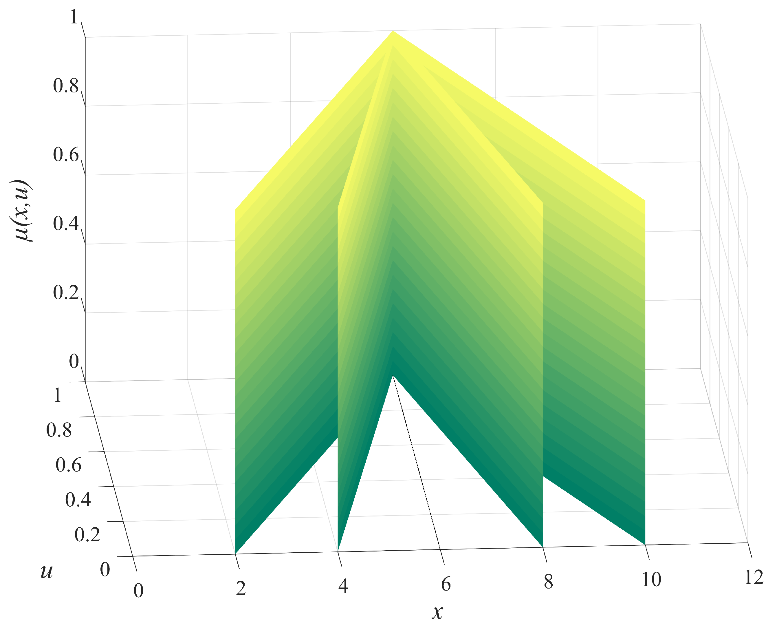
Example 1.

An RSTIT2-FV A = $\left(\begin{array}{ccc}2& 6& 10\\ 4& 6& 8\end{array}\right)$ is visualized in Figure 1.

Afterwards, Li and Cai [27] defined the medium of an RSTIT2-FV by means of the UMF and LMF to avoid the uncertainty of the membership functions in an uncertain and convoluted context. Then according to the membership function of the medium, they derived the credibility distribution of an RSTIT2-FV.

Definition 11.

(Li and Cai [27]) Given that Z is an RSTIT2-FV, ζ is a T1-FV. If their membership functions conform to:

$${\mu }_{\zeta }\left(x\right)=\frac{1}{2}UMF+\frac{1}{2}LMF,$$

then ζ is called the medium of Z, and ${\mu }_{\zeta }\left(x\right)$ can be calculated by:

$${\mu }_{\zeta }\left(x\right)=\left\{\begin{array}{cc}{\displaystyle \frac{1}{2}}\left({\displaystyle \frac{1}{l_U}}x-{\displaystyle \frac{c-l_U}{l_U}}\right),\hfill & x\in [c-l_U,c-l_L)\hfill \\ {\displaystyle \frac{1}{2}}\left({\displaystyle \frac{1}{l_U}}x-{\displaystyle \frac{c-l_U}{l_U}}\right)+{\displaystyle \frac{1}{2}}\left({\displaystyle \frac{1}{l_L}}x-{\displaystyle \frac{c-l_L}{l_L}}\right),\hfill & x\in [c-l_L,c)\hfill \\ {\displaystyle \frac{1}{2}}\left(-{\displaystyle \frac{1}{l_U}}x+{\displaystyle \frac{c+l_U}{l_U}}\right)+{\displaystyle \frac{1}{2}}\left(-{\displaystyle \frac{1}{l_L}}x+{\displaystyle \frac{c+l_L}{l_L}}\right),\hfill & x\in [c,c+l_L)\hfill \\ {\displaystyle \frac{1}{2}}\left(-{\displaystyle \frac{1}{l_U}}x+{\displaystyle \frac{c+l_U}{l_U}}\right),\hfill & x\in [c+l_L,c+l_U]\hfill \\ 0,\hfill & otherwise.\hfill \end{array}\right.$$

(3)

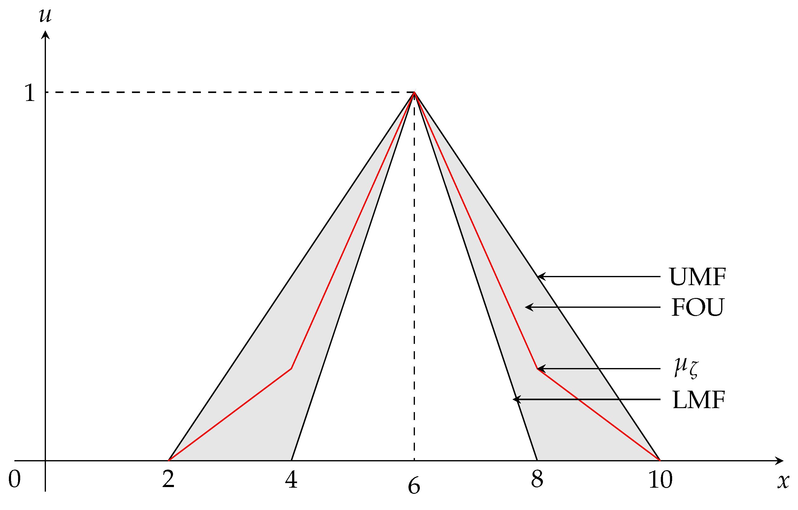
Example 2.

For the RSTIT2-FV in Example 1, the membership function of its medium ${\zeta }_1$ is depicted as the red line in Figure 2.

2.3. The Credibility Distribution of the RSTIT2-FV

Li and Cai [27] defined the credibility distribution with the membership function of the medium $\zeta$. Then they derived the inverse credibility distribution of the RSTIT2-FV.

Definition 12.

(Li and Cai [27]) Given that Z is an RSTIT2-FV, B is a fuzzy event of the universe, and ζ is the medium of Z. Then $Pos$, $Nec$ and $Cr$ represents the possibility, necessity and credibility measures, respectively,

$$\begin{array}{cc}\hfill & \mathrm{Pos}\left\{B\right\}={\sup }_{x\in B}{\mu }_{\zeta }\left(x\right),\hfill \\ \hfill & \mathrm{Nec}\left\{B\right\}=1-{\sup }_{x\in B^c}{\mu }_{\zeta }\left(x\right),\hfill \\ \hfill & \mathrm{Cr}\left\{B\right\}=\frac{1}{2}\left(\mathrm{Pos}\left\{B\right\}+\mathrm{Nec}\left\{B\right\}\right).\hfill \end{array}$$

Theorem 1.

(Li and Cai [27]) The credibility measure for a fuzzy event B of an RSTIT2-FV complies with the formulation as below

$$\mathrm{Cr}\left\{B\right\}+\mathrm{Cr}\left\{B^c\right\}=1.$$

Definition 13.

(Li and Cai [27])Let Z be an RSTIT2-FV, and ζ be the medium of Z, then the credibility distribution of Z, ${\Phi }_Z$, is formulated by:

$$\begin{array}{cc}\hfill {\Phi }_Z\left(x\right)& =\mathrm{Cr}\{Z\le x\}\hfill \\ \hfill & =\left\{\begin{array}{cc}0,\hfill & x\in (-\infty ,c-l_U]\hfill \\ {\displaystyle \frac{1}{4}}\left({\displaystyle \frac{1}{l_U}}x-{\displaystyle \frac{c-l_U}{l_U}}\right),\hfill & x\in (c-l_U,c-l_L]\hfill \\ {\displaystyle \frac{1}{4}}\left({\displaystyle \frac{1}{l_U}}x-{\displaystyle \frac{c-l_U}{l_U}}\right)+{\displaystyle \frac{1}{4}}\left({\displaystyle \frac{1}{l_L}}x-{\displaystyle \frac{c-l_L}{l_L}}\right),\hfill & x\in (c-l_L,c+l_L]\hfill \\ 1+{\displaystyle \frac{1}{4}}\left({\displaystyle \frac{1}{l_U}}x-{\displaystyle \frac{c+l_U}{l_U}}\right),\hfill & x\in (c+l_L,c+l_U]\hfill \\ 1,\hfill & x\in (c+l_U,+\infty ).\hfill \end{array}\right.\hfill \end{array}$$

(4)

The inverse credibility distribution of Z, ${\Phi }_Z^{-1}$, is:

$${\Phi }_Z^{-1}\left(\alpha \right)=\left\{\begin{array}{cc}4l_U\alpha +c-l_U,\hfill & \alpha \in \left[0,{\displaystyle \frac{l_U-l_L}{4l_U}}\right)\hfill \\ {\displaystyle \frac{4l_U{l}_L\alpha -2l_U{l}_L}{l_U+l_L}}+c,\hfill & \alpha \in \left[{\displaystyle \frac{l_U-l_L}{4l_U}},1-{\displaystyle \frac{l_U-l_L}{4l_U}}\right)\hfill \\ 4l_U\alpha +c-3l_U,\hfill & \alpha \in \left[1-{\displaystyle \frac{l_U-l_L}{4l_U}},1\right].\hfill \end{array}\right.$$

(5)

Theorem 2.

(Li and Cai [27]) Suppose that there are RSTIT2-FVs $Z_i$ which are mutually independent, and ${\zeta }_i$ are the mediums of $Z_i$ respectively, i $=1,2,\dots ,m,$ when $f\left(x_1,\dots ,x_k,x_{k+1},\dots ,x_m\right)$ is strictly increasing towards $x_i,i=1,2,\dots$, k, and strictly decreasing towards $x_i,i=k+1,k+2,\dots ,m$, then the inverse credibility distribution of

$$Z=f\left(Z_1,\cdots ,Z_k,Z_{k+1},\cdots ,Z_m\right)$$

is formulated as

$${\Phi }_Z^{-1}\left(\alpha \right)=f\left({\Phi }_{Z_1}^{-1}\left(\alpha \right),\cdots ,{\Phi }_{Z_k}^{-1}\left(\alpha \right),{\Phi }_{Z_{k+1}}^{-1}(1-\alpha ),\cdots ,{\Phi }_{Z_m}^{-1}(1-\alpha )\right).$$

(6)

2.4. The Expected Value, Variance and Semi-Variances of the Fuzzy Variable

Definition 14.

(Liu [32]) Suppose that Z is a fuzzy variable and its expected value is ε, then its variance can be formulated as:

$$V\left[Z\right]=E\left[{(Z-\epsilon )}^2\right].$$

(7)

Definition 15.

(Liu [28]) Suppose that Z is a fuzzy variable, then the expected value of Z can be formulated as:

$$E\left[Z\right]={\int }_0^{+\infty }Cr\left\{Z\ge x\right\}\mathrm{d}x-{\int }_{-\infty }^{0}Cr\left\{Z\le x\right\}dx.$$

(8)

Theorem 3.

(Liu [33]) Given that Z is an fuzzy variable, then its expected value can be reformed to:

$$E\left[Z\right]={\int }_0^1{\Phi }_Z^{-1}\left(\alpha \right)\mathrm{d}\alpha .$$

(9)

Specifically, for an RSTIT2-FV, Li and Cai [27] has proved that its expected value is identical to the center value, that is, $E\left[Z\right]=\epsilon$.

Theorem 4.

(Li and Cai [27]) Given that Z = $\left(\begin{array}{ccc}c-l_U& c& c+l_U\\ c-l_L& c& c+l_L\end{array}\right)$ is an RSTIT2-FV with the center value c and the inverse credibility distribution ${\Phi }_Z^{-1}\left(\alpha \right)$, then its expected value is identical to c, that is,

$$E\left[Z\right]={\int }_0^1{\Phi }_Z^{-1}\left(\alpha \right)\mathrm{d}\alpha =c.$$

(10)

Theorem 5.

(Li and Cai [27]) Suppose that Z is an RSTIT2-FV and k is a constant, then

$$E\left[kZ\right]=kE\left[Z\right].$$

(11)

Definition 16.

(Gu et al. [8]) Suppose that Z is a fuzzy variable and its expected value is ε, then the upside semi-variance of Z can be formulated as:

$$S{v}^{+}\left[Z\right]=E\left[{\left({(Z-\epsilon )}^{+}\right)}^2\right],$$

(12)

where

$${(Z-\epsilon )}^{+}=\left\{\begin{array}{cc}Z-\epsilon ,\hfill & if\mathrm{Z}>\epsilon \hfill \\ 0,\hfill & ifZ\le \epsilon .\hfill \end{array}\right.$$

Definition 17.

(Huang [34]) Suppose that Z is a fuzzy variable and its expected value is ε, then the downside semi-variance of Z can be formulated as:

$$S{v}^{-}\left[Z\right]=E\left[{\left({(Z-\epsilon )}^{-}\right)}^2\right],$$

(13)

where

$${(Z-\epsilon )}^{-}=\left\{\begin{array}{cc}0,\hfill & ifZ>\epsilon \hfill \\ Z-\epsilon ,\hfill & ifZ\le \epsilon .\hfill \end{array}\right.$$

In the following sections, the variance and semi-variances for the RIT2-FV as well as the covariance and operational law for the RSTIT2-FV will be defined.

3. The Variance of the RIT2-FV

We will provide the calculation formula for the variance of an RIT2-FV via the credibility distribution in this section, which can be derived by Definitions 14 and 15.

Definition 18.

Let Z be an RIT2-FV and its expected value is ε, then its variance is formulated as:

$$V\left[Z\right]=E\left[{(Z-\epsilon )}^2\right].$$

(14)

Definition 19.

Let Z be an RIT2-FV, then the expected value of Z can be formulated as:

$$E\left[Z\right]={\int }_0^{+\infty }Cr\left\{Z\ge x\right\}\mathrm{d}x-{\int }_{-\infty }^{0}Cr\left\{Z\le x\right\}dx.$$

(15)

Theorem 6.

Given that Z is an RIT2-FV. Then ${\Phi }_Z\left(x\right)$ is the credibility distribution of Z and ε is the expected value of Z. Its variance can be calculated by:

$$V\left[Z\right]={\int }_0^{+\infty }\left[1-{\Phi }_Z(\epsilon +\sqrt{x})+{\Phi }_Z(\epsilon -\sqrt{x})\right]dx.$$

(16)

Proof. 

On the basis of Definitions 18 and 19, we derive:

$$\begin{array}{cc}\hfill V\left[Z\right]=E\left[{(Z-\epsilon )}^2\right]& ={\int }_0^{+\infty }Cr\left\{{(Z-\epsilon )}^2\ge x\right\}\mathrm{d}x-{\int }_{-\infty }^{0}Cr\left\{{(Z-\epsilon )}^2\le x\right\}dx\hfill \\ & ={\int }_0^{+\infty }Cr\{\{Z\ge \sqrt{x}+\epsilon \}\cup \{Z\le \epsilon -\sqrt{x}\}\}\hfill \\ & ={\int }_0^{+\infty }\left[1-{\Phi }_Z(\epsilon +\sqrt{x})+{\Phi }_Z(\epsilon -\sqrt{x})\right]dx.\hfill \end{array}$$

Thus, Equation (16) is naturally obtained. □

Remark 1.

For an RSTIT2-FV Z= $\left(\begin{array}{ccc}c-l_U& c& c+l_U\\ c-l_L& c& c+l_L\end{array}\right)$, the formula for calculating its variance can be simplified as:

$$\begin{array}{cc}\hfill V\left[Z\right]=& {\int }_0^{+\infty }\left[1-{\Phi }_Z(\epsilon +\sqrt{x})+{\Phi }_Z(\epsilon -\sqrt{x})\right]dx\hfill \\ \hfill =& {\int }_0^{l_L^2}\left(1-\frac{\sqrt{x}}{4l_U}-\frac{\sqrt{x}}{4l_L}-\frac{1}{2}+\frac{1}{2}-\frac{\sqrt{x}}{4l_U}-\frac{\sqrt{x}}{4l_L}\right)dx\hfill \\ \hfill & +{\int }_{l_L^2}^{l_U^2}\left[1-1-\frac{1}{4}\left(\frac{\sqrt{x}}{l_U}-1\right)+\frac{1}{4}\left(1-\frac{\sqrt{x}}{l_U}\right)\right]dx\hfill \\ \hfill =& \frac{1}{6}\left(l_L^2+l_U^2\right).\hfill \end{array}$$

(17)

Example 3.

For two RSTIT2-FVs A = $\left(\begin{array}{ccc}2& 6& 10\\ 4& 6& 8\end{array}\right)$ and B = $\left(\begin{array}{ccc}2& 5& 8\\ 3& 5& 7\end{array}\right)$, we can easily obtain their variances by Equation (17) as:

$$V\left[A\right]=\frac{1}{6}\left(2^2+4^2\right)=\frac{10}{3},V\left[B\right]=\frac{1}{6}\left(2^2+3^2\right)=\frac{13}{6}.$$

Theorem 7.

Given that Z is an RIT2-FV. Then ${\Phi }_Z\left(x\right)$ is the credibility distribution of Z and ε is the expected value of Z. Its variance can be calculated by:

$$V\left[Z\right]={\int }_0^1\left[{\Phi }_Z^{-1}\left(\alpha \right)-\epsilon \right]dx,$$

(18)

where ${\Phi }_Z^{-1}\left(\alpha \right)$ is the inverse credibility distribution of Z.

Proof. 

Following from Theorem 6, the part of ${\int }_0^{+\infty }\left[1-{\Phi }_Z(\epsilon +\sqrt{x})\right]dx$ of Equation (16) can be transformed to:

$${\int }_0^{+\infty }\left[1-{\Phi }_Z(\epsilon +\sqrt{x})\right]dx={\int }_{{\Phi }_Z\left(\epsilon \right)}^1(1-\alpha )d{\left[{\Phi }_Z^{-1}\left(\alpha \right)-\epsilon \right]}^2={\int }_{{\Phi }_Z\left(\epsilon \right)}^1\left[{\Phi }_Z^{-1}\left(\alpha \right)-\epsilon \right]d\alpha$$

by replacing ${\Phi }_Z(\epsilon +\sqrt{x})$ with $\alpha$. Similarly, the part of ${\int }_0^{+\infty }{\Phi }_s(\epsilon -\sqrt{x})dx$ can be transformed to:

$${\int }_0^{+\infty }{\Phi }_Z(\epsilon -\sqrt{x})dx={\int }_{{\Phi }_Z\left(\epsilon \right)}^0\alpha d{\left[\epsilon -{\Phi }_Z^{-1}\left(\alpha \right)\right]}^2={\int }_0^{{\Phi }_Z\left(\epsilon \right)}\left[{\Phi }_Z^{-1}\left(\alpha \right)-\epsilon \right]d\alpha$$

by replacing ${\Phi }_s(\epsilon -\sqrt{x})$ with $\alpha$. Hence, we obtain:

$$\begin{array}{cc}\hfill V\left[Z\right]& ={\int }_0^{+\infty }\left[1-{\Phi }_Z(\epsilon +\sqrt{x})+{\Phi }_Z(\epsilon -\sqrt{x})\right]dx\hfill \\ & ={\int }_{{\Phi }_Z\left(\epsilon \right)}^1\left[{\Phi }_Z^{-1}\left(\alpha \right)-\epsilon \right]d\alpha +{\int }_0^{{\Phi }_Z\left(\epsilon \right)}\left[{\Phi }_Z^{-1}\left(\alpha \right)-\epsilon \right]d\alpha \hfill \\ & ={\int }_0^1\left[{\Phi }_Z^{-1}\left(\alpha \right)-\epsilon \right]dx.\hfill \end{array}$$

 □

4. The Semi-Variances of an RIT2-FV

In the previous section, we have derived the calculation formula for the variance of the RIT2-FVs, which indicates bilateral deviation of variables. In practice, however, such as stock portfolio selection, we focus on the negative deviation to measure the risk in loss; and in R&D investment, only the positive deviation is used to control the cost. Such deviations can be measured by one-side semi-variances respectively.

Thus, we define the formulas for the downside and upside semi-variances of the RIT2-FV according to the credibility distribution (Gu et al. [8] and Huang [34]) in the following. After that, the relationships between the variance and semi-variances are uncovered.

4.1. Calculation Formula for the Semi-Variances of the RIT2-FV

Theorem 8.

Given that Z is an RIT2-FV. Then ${\Phi }_Z\left(x\right)$ is the credibility distribution of Z and ε is the expected value of Z. The upside semi-variance can be formulated as:

$$S{v}^{+}\left[Z\right]={\int }_0^{+\infty }\left[1-{\Phi }_Z(\epsilon +\sqrt{x})\right]dx.$$

(19)

Proof. 

According to Definitions 16 and 19, we have:

$$\begin{array}{cc}\hfill S{v}^{+}\left[Z\right]& =E\left[{\left({(Z-\epsilon )}^{+}\right)}^2\right]\hfill \\ & ={\int }_0^{+\infty }Cr\left\{{(Z-\epsilon )}^2\ge x,Z>\epsilon \right\}dx\hfill \\ & ={\int }_0^{+\infty }Cr\{Z\ge \epsilon +\sqrt{x}\}dx\hfill \\ & ={\int }_0^{+\infty }\left[1-{\Phi }_Z(\epsilon +\sqrt{x})\right]dx.\hfill \end{array}$$

 □

Theorem 9.

Given that Z is an RIT2-FV. Then ${\Phi }_Z\left(x\right)$ is the credibility distribution of Z and ε is the expected value of Z. The downside semi-variance can be formulated as:

$$S{v}^{-}\left[Z\right]={\int }_0^{+\infty }{\Phi }_Z(\epsilon -\sqrt{x})dx.$$

(20)

Proof. 

Similar to Proof of Theorem 8, in light of Definitions 17 and 19, we have:

$$\begin{array}{cc}\hfill S{v}^{-}\left[Z\right]& =E\left[{\left({(Z-\epsilon )}^{-}\right)}^2\right]\hfill \\ & ={\int }_0^{+\infty }Cr\left\{{(Z-\epsilon )}^2\ge x,Z\le \epsilon \right\}dx\hfill \\ & ={\int }_0^{+\infty }Cr\{Z\le \epsilon -\sqrt{x}\}dx\hfill \\ & ={\int }_0^{+\infty }{\Phi }_Z(\epsilon -\sqrt{x})dx.\hfill \end{array}$$

 □

Remark 2.

Given that Z = $\left(\begin{array}{ccc}c-l_U& c& c+l_U\\ c-l_L& c& c+l_L\end{array}\right)$ is an RSTIT2-FV. Then ${\Phi }_Z\left(x\right)$ is the credibility distribution of Z and ε is the expected value of Z. By means of Theorems 8 and 9, the formula for calculating the upside and downside semi-variance of Z can be simplified as:

$$\begin{array}{cc}\hfill S{v}^{+}\left[Z\right]& ={\int }_0^{+\infty }\left[1-{\Phi }_Z(\epsilon +\sqrt{x})\right]dx\hfill \\ \hfill & ={\int }_0^{l_L^2}\left[1-\frac{1}{4}\left(\frac{\sqrt{x}}{l_U}+\frac{\sqrt{x}}{l_L}+2\right)\right]dx+\frac{1}{4}{\int }_{l_L^2}^{l_U^2}\left(1-\frac{\sqrt{x}}{l_U}\right)dx\hfill \\ \hfill & =\frac{1}{12}\left(l_L^2+l_U^2\right)\hfill \end{array}$$

(21)

and

$$\begin{array}{cc}\hfill S{v}^{-}\left[Z\right]& ={\int }_0^{+\infty }{\Phi }_Z(\epsilon -\sqrt{x})dx\hfill \\ \hfill & =-\frac{1}{4}{\int }_0^{l_L^2}\left(\frac{\sqrt{x}}{l_U}+\frac{\sqrt{x}}{l_L}+2\right)dx+\frac{1}{4}{\int }_{l_L^2}^{l_U^2}\left(1-\frac{\sqrt{x}}{l_U}\right)dx\hfill \\ \hfill & =\frac{1}{12}\left(l_L^2+l_U^2\right).\hfill \end{array}$$

(22)

Example 4.

By using Equations (21) and (22), the upside and downside semi-variances of the two RSTIT2-FVs in Example 3 can be derived as:

$$S{v}^{+}\left[A\right]=S{v}^{-}\left[A\right]=\frac{1}{12}\left(2^2+4^2\right)=\frac{5}{3}$$

and

$$S{v}^{+}\left[B\right]=S{v}^{-}\left[B\right]=\frac{1}{12}\left(2^2+3^2\right)=\frac{13}{12}.$$

4.2. The Relationships between the Variance and Semi-Variances

In the above sections, we deduce the formulae for calculating the variance and semi-variances of the RIT2-FV based on the credibility distribution. In this section, we further probe into the relationship between the variance and semi-variances of the RSTIT2-FV.

Observed from the Equations (13), (16) and (19), the semi-variance is equal to parts of the formula for calculating the variance. We find that there exist some relationships between the variance and semi-variances of the RSTIT2-FV.

Theorem 10.

Suppose that Z is an RSTIT2-FV, then its upside and downside semi-variances and variance satisfy:

$$V\left[Z\right]=S{v}^{+}\left[Z\right]+S{v}^{-}\left[Z\right].$$

(23)

Proof. 

In light of Equations (19) and (20), we have:

$$\begin{array}{c}\hfill S{v}^{+}\left[Z\right]+S{v}^{-}\left[Z\right]={\int }_0^{+\infty }\left[1-{\Phi }_Z(\epsilon +\sqrt{x})+{\Phi }_Z(\epsilon -\sqrt{x})\right]dx,\end{array}$$

which is equal to $V\left[Z\right]$ in Equation (9). Therefore, we have:

$$V\left[Z\right]=S{v}^{+}\left[Z\right]+S{v}^{-}\left[Z\right].$$

 □

It can also be observed from Equations (21) and (22) that $S{v}^{-}\left[Z\right]=S{v}^{+}\left[Z\right]$. Thus, we can derive the following theorem regarding the relationship between them.

Theorem 11.

Let Z be an RSTIT2-FV, then its upside and downside semi-variances satisfy:

$$S{v}^{-}\left[Z\right]=S{v}^{+}\left[Z\right].$$

(24)

Proof. 

For an RSTIT2-FV Z = $\left(\begin{array}{ccc}c-l_U& c& c+l_U\\ c-l_L& c& c+l_L\end{array}\right)$, we can obtain that its expected value $\epsilon$ is identical to c. Then, in view of Definitions 16 and 17, its downside and upside semi-variances are, respectively,

$$\begin{array}{cc}\hfill S{v}^{+}& ={\int }_0^{+\infty }Cr\{Z\le \epsilon -\sqrt{t}\}dt,\hfill \\ \hfill S{v}^{-}& ={\int }_0^{+\infty }Cr\{Z\ge \epsilon +\sqrt{t}\}dt.\hfill \end{array}$$

From Definition 12, we can obtain

$$Cr\{Z\le t\}=\frac{1}{2}\left(\begin{array}{c}\left.{\sup }_{x\le t}\mu \left(x\right)+1-{\sup }_{x>t}\mu \left(x\right)\right),\hfill \end{array}\right.$$

Thereforth,

$$Cr\{Z\le \epsilon -\sqrt{t}\}=\frac{1}{2}\left[{\sup }_{x\le \epsilon -\sqrt{t}}{\mu }_Z\left(x\right)+1-{\sup }_{x>\epsilon -\sqrt{t}}{\mu }_Z\left(x\right)\right].$$

For $\epsilon -\sqrt{t}\le \epsilon$, ${\sup }_{x>\epsilon -\sqrt{t}}{\mu }_Z\left(x\right)=1.$ Thus,

$$Cr\{Z\le \epsilon -\sqrt{t}\}=\frac{1}{2}{\sup }_{x\le \epsilon -\sqrt{t}}{\mu }_Z\left(x\right)=\frac{1}{2}Pos\{Z\le \epsilon -\sqrt{t}\}.$$

Analogonsly, we can derive that

$$Cr\{Z\ge \epsilon +\sqrt{t}\}=\frac{1}{2}Pos\{Z\ge \epsilon +\sqrt{t}\}.$$

Since Z is a sysmetric fuzzy variable, it can be conveniently deduced that

$$Pos\{Z\le \epsilon -\sqrt{t}\}=Pos\{Z\ge \epsilon +\sqrt{t}\}.$$

Eventually, we can obtain that:

$$S{v}^{-}\left[Z\right]=S{v}^{+}\left[Z\right].$$

 □

Theorem 12.

Suppose that Z is an RSTIT2-FV, then its upside and downside semi-variances and variance satisfy:

$$S{v}^{+}\left[Z\right]=S{v}^{-}\left[Z\right]=\frac{1}{2}V\left[Z\right].$$

(25)

Proof. 

According to Theorems 10 and 11, we have:

$$V\left[Z\right]=S{v}^{+}\left[Z\right]+S{v}^{-}\left[Z\right]$$

and

$$S{v}^{-}\left[Z\right]=S{v}^{+}\left[Z\right].$$

Therefore, it can be readily deducted that:

$$S{v}^{+}\left[Z\right]=S{v}^{-}\left[Z\right]=\frac{1}{2}V\left[Z\right].$$

 □

According to Theorem 11, the upside and downside semi-variances of an RSTIT2-FV are equal to each other. Therefore, in the following section, they are collectively referred to as the semi-variance and denoted as $Sv\left[Z\right]$.

5. Operational Law

This section introduces the calculated operational law of the variance and semi-variance for the RSTIT2-FV. The definition of independence, as a precondition for its derivation, is referred to in the beginning.

5.1. Independence

Definition  20.

(Li and Cai [27]) The RSTIT2-FVs $Z_i,i=1,2,\cdots ,m$, are said to be mutually independent if:

$$\mathrm{Cr}\{Z_i\in A_i,i=1,2,\cdots ,m\}=\underset{1\le i\le m}{min}\mathrm{Cr}\{Z_i\in B_i\},$$

for any subsets $B_1,B_2,\cdots ,B_m$.

Theorem 13.

(Li and Cai [27]) If the RSTIT2-FVs $Z_i,i=1,2,\cdots ,m$, are mutually independent, then their corresponding mediums ${\zeta }_i$ are mutually independent as well.

5.2. Operational Law for the RSTIT2-FVs

Theorem 14.

Let Z be an RSTIT2-FV. k is a constant and ε is the expected value of Z, then we have:

$$V\left[kZ\right]=k^{2}V\left[Z\right].$$

(26)

Proof. 

According to Definition 18 and Theorem 5, we have:

$$\begin{array}{c}\hfill V\left[kZ\right]=E\left[{(kZ-kE\left[Z\right])}^2\right]=E\left[{(kZ-k\epsilon )}^2\right]=k^{2}E\left[{(Z-\epsilon )}^2\right]=k^{2}V\left[Z\right].\end{array}$$

 □

Definition 21.

Let $Z_1$ and $Z_2$ be two mutually independent RSTIT2-FVs with expected value ${\epsilon }_1$ and ${\epsilon }_2$, respectively. Then, the covariance of $Z_1$ and $Z_2$ is formulated as:

$$Cov\left[Z_1,Z_2\right]=E\left[\left(Z_1-{\epsilon }_1\right)\left(Z_2-{\epsilon }_2\right)\right].$$

(27)

In view of the subadditivity of the uncertain measure, the covariance of the RSTIT2-FVs cannot be calculated straightly by means of their credibility distributions. By comparing Definitions 18 and 21, variance can be regarded as a specific kind of covariance. Therefore, we can derive the formula for calculating the covariance via the inverse credibility distribution, in view of Equation (18).

Stipulation 1.

Let $Z_1$ and $Z_2$ are two mutually independent RSTIT2-FVs with distributions ${\Phi }_{Z_1}$ and ${\Phi }_{Z_2}$ and expected value ${\epsilon }_1$ and ${\epsilon }_2$ respectively. Then the covariance of $Z_1$ and $Z_2$ is:

$$Cov[Z_1,Z_2]={\int }_0^1\left[{\Phi }_{Z_1}^{-1}\left(\alpha \right)-{\epsilon }_1\right]\left[{\Phi }_{Z_2}^{-1}\left(\alpha \right)-{\epsilon }_2\right]dx.$$

(28)

Theorem 15.

Suppose that $Z_1$ and $Z_2$ are two mutually independent RSTIT2-FVs with the credibility distributions ${\Phi }_{Z_1}$ and ${\Phi }_{Z_2}$ and expected value ${\epsilon }_1$ and ${\epsilon }_2$, respectively, then the covariance of $Z_1$ and $Z_2$ is:

$${\displaystyle Cov[Z_1,Z_2]={\int }_0^1{\Phi }_{Z_1}^{-1}\left(\alpha \right){\Phi }_{Z_2}^{-1}\left(\alpha \right)\mathrm{d}\alpha -{\epsilon }_1{\epsilon }_2.}$$

(29)

Proof. 

In light of Stipulation 1, the covariance of $Z_1$ and $Z_2$ is conveniently derived as:

$$\begin{array}{cc}\hfill Cov[Z_1,Z_2]& {\displaystyle ={\int }_0^1\left({\Phi }_{Z_1}^{-1}\left(\alpha \right){\Phi }_{Z_2}^{-1}\left(\alpha \right)-{\epsilon }_2{\Phi }_{Z_1}^{-1}\left(\alpha \right)-{\epsilon }_1{\Phi }_{Z_2}^{-1}\left(\alpha \right)+{\epsilon }_1{\epsilon }_2\right)\mathrm{d}\alpha }\hfill \\ & {\displaystyle ={\int }_0^1{\Phi }_{Z_1}^{-1}\left(\alpha \right){\Phi }_{Z_2}^{-1}\left(\alpha \right)\mathrm{d}\alpha -{\epsilon }_2{\int }_0^1{\Phi }_{Z_1}^{-1}\left(\alpha \right)\mathrm{d}\alpha -{\epsilon }_1{\int }_0^1{\Phi }_{Z_2}^{-1}\left(\alpha \right)\mathrm{d}\alpha +{\epsilon }_1{\epsilon }_2.}\hfill \end{array}$$

Then according to Equation (9), we get:

$${\displaystyle Cov[Z_1,Z_2]={\int }_0^1{\Phi }_{Z_1}^{-1}\left(\alpha \right){\Phi }_{Z_2}^{-1}\left(\alpha \right)\mathrm{d}\alpha -{\epsilon }_1{\epsilon }_2.}$$

 □

Example 5.

For two mutually independent RSTIT2-FVs A and B in Example 3 with the inverse credibility distributions,

$$\begin{array}{c}\hfill {\Phi }_A^{-1}\left(\alpha \right)=\left\{\begin{array}{cc}16\alpha +2,\hfill & \alpha \in \left[0,{\displaystyle \frac{1}{8}}\right)\hfill \\ {\displaystyle \frac{16\alpha +10}{3}},\hfill & \alpha \in \left[{\displaystyle \frac{1}{8}},{\displaystyle \frac{7}{8}}\right)\hfill \\ 16\alpha -6,\hfill & \alpha \in \left[{\displaystyle \frac{7}{8}},1\right]\hfill \end{array}\right.\end{array}$$

and

$${\Phi }_B^{-1}\left(\alpha \right)=\left\{\begin{array}{cc}12\alpha +2,\hfill & \alpha \in \left[0,{\displaystyle \frac{1}{12}}\right)\hfill \\ {\displaystyle \frac{24\alpha +13}{5}},\hfill & \alpha \in \left[{\displaystyle \frac{1}{12}},{\displaystyle \frac{11}{12}}\right)\hfill \\ 12\alpha -4,\hfill & \alpha \in \left[{\displaystyle \frac{11}{12}},1\right]\hfill \end{array}\right.,$$

respectively, their covariance is:

$$\begin{array}{cc}\hfill Cov[A,B]=& {\int }_0^1{\Phi }_A^{-1}\left(\alpha \right){\Phi }_B^{-1}\left(\alpha \right)d\alpha -{\epsilon }_1{\epsilon }_2\hfill \\ \hfill =& {\int }_0^{\frac{1}{12}}(16\alpha +2)(12\alpha +2)d\alpha +{\int }_{\frac{1}{12}}^{\frac{1}{8}}\frac{(24\alpha +13)(16\alpha +2)}{5}d\alpha \hfill \\ & +{\int }_{\frac{1}{8}}^{\frac{7}{8}}\frac{(16a+10)(24\alpha +13)}{15}d\alpha +{\int }_{\frac{7}{8}}^{\frac{11}{12}}\frac{(16\alpha -6)(24\alpha +13)}{5}d\alpha \hfill \\ & +{\int }_{\frac{11}{12}}^1(12\alpha -4)(16\alpha -6)d\alpha -6\times 5\hfill \\ \hfill =& \frac{61}{108}+\frac{64}{135}+\frac{117}{5}+\frac{647}{270}+\frac{631}{108}-30\hfill \\ \hfill =& \frac{241}{90}.\hfill \end{array}$$

Theorem 16.

Suppose that $Z_1$ and $Z_2$ are two mutually independent RSTIT2-FVs with expected values ${\epsilon }_1$ and ${\epsilon }_2$, respectively, then the variance of $k_1{Z}_1+k_2{Z}_2$ is

$$V\left[k_1{Z}_1+k_2{Z}_2\right]=k_1^{2}V\left[Z_1\right]+k_2^{2}V\left[Z_2\right]+2k_1{k}_{2}Cov\left[Z_1,Z_2\right],$$

(30)

where the constants $k_1$ and $k_2$ satisfy $k_1{k}_2>0$.

Proof. 

According to Theorem 7, the variance of $k_1{Z}_1+k_2{Z}_2$ can be calculated by:

$$V\left[k_1{Z}_1+k_2{Z}_2\right]={\int }_0^1{\left[{\Phi }_{k_1{Z}_1+k_2{Z}_2}^{-1}\left(\alpha \right)-\mathrm{E}\left[k_1{Z}_1+k_2{Z}_2\right]\right]}^{2}d\alpha .$$

(31)

When $k_1>0$ and $k_2>0$, $k_1{Z}_1+k_2{Z}_2$ is strictly increasing with respect to $Z_1$ and $Z_2$. In light of Theorem 2, the inverse credibility distribution of $k_1{Z}_1+k_2{Z}_2$ is:

$${\Phi }_{k_1{Z}_1+k_2{Z}_2}^{-1}\left(\alpha \right)=k_1{\Phi }_{Z_1}^{-1}\left(\alpha \right)+k_2{\Phi }_{Z_2}^{-1}\left(\alpha \right).$$

So following from Equation (31):

$$\begin{array}{cc}\hfill V\left[k_1{Z}_1+k_2{Z}_2\right]=& {\int }_0^1{\left[k_1{\Phi }_{Z_1}^{-1}\left(\alpha \right)+k_2{\Phi }_{Z_2}^{-1}\left(\alpha \right)-\mathrm{E}\left[k_1{Z}_1+k_2{Z}_2\right]\right]}^{2}d\alpha \hfill \\ \hfill =& {\int }_0^1{k}_1^2{\left({\Phi }_{Z_1}^{-1}\left(\alpha \right)-{\epsilon }_1\right)}^2+k_2^2{\left({\Phi }_{Z_2}^{-1}\left(\alpha \right)-{\epsilon }_2\right)}^2\hfill \\ & +2k_1{k}_2\left({\Phi }_{Z_1}^{-1}\left(\alpha \right)-{\epsilon }_1\right)\left({\Phi }_{Z_2}^{-1}\left(\alpha \right)-{\epsilon }_2\right)d\alpha \hfill \\ \hfill =& k_1^{2}V\left[Z_1\right]+k_2^{2}V\left[Z_2\right]+2k_1{k}_{2}Cov\left[Z_1,Z_2\right].\hfill \end{array}$$

When $k_1<0$ and $k_2<0$, $k_1{Z}_1+k_2{Z}_2$ is strictly decreasing with respect to $Z_1$ and $Z_2$. In light of Theorem 16, the inverse credibility distribution of $k_1{Z}_1+k_2{Z}_2$ is:

$${\Phi }_{k_1{Z}_1+k_2{Z}_2}^{-1}\left(\alpha \right)=k_1{\Phi }_{Z_1}^{-1}(1-\alpha )+k_2{\Phi }_{Z_2}^{-1}(1-\alpha ).$$

Then according to Equation (31), we have:

$$\begin{array}{cc}\hfill V\left[k_1{Z}_1+k_2{Z}_2\right]=& {\int }_0^1{\left[k_1{\Phi }_{Z_1}^{-1}(1-\alpha )+k_2{\Phi }_{Z_2}^{-1}(1-\alpha )-\mathrm{E}\left[k_1{Z}_1+k_2{Z}_2\right]\right]}^{2}d\alpha \hfill \\ \hfill =& {\int }_0^1{k}_1^2{\left({\Phi }_{Z_1}^{-1}(1-\alpha )-{\epsilon }_1\right)}^2+k_2^2{\left({\Phi }_{Z_2}^{-1}(1-\alpha )-{\epsilon }_2\right)}^2\hfill \\ & +2k_1{k}_2\left({\Phi }_{Z_1}^{-1}(1-\alpha )-{\epsilon }_1\right)\left({\Phi }_{Z_2}^{-1}(1-\alpha )-{\epsilon }_2\right)d\alpha .\hfill \end{array}$$

By replacing $(1-\alpha )$ with $\beta$, we obtain that:

$$\begin{array}{cc}\hfill V\left[k_1{Z}_1+k_2{Z}_2\right]=& {\int }_0^1{k}_1^2{\left({\Phi }_{Z_1}^{-1}\left(\beta \right)-{\epsilon }_1\right)}^2+k_2^2{\left({\Phi }_{Z_2}^{-1}\left(\beta \right)-{\epsilon }_2\right)}^2\hfill \\ & +2k_1{k}_2\left({\Phi }_{Z_1}^{-1}\left(\beta \right)-{\epsilon }_1\right)\left({\Phi }_{Z_2}^{-1}\left(\beta \right)-{\epsilon }_2\right)d\beta \hfill \\ \hfill =& k_1^{2}V\left[Z_1\right]+k_2^{2}V\left[Z_2\right]+2k_1{k}_{2}Cov\left[Z_1,Z_2\right].\hfill \end{array}$$

 □

Example 6.

For the two mutually independent RSTIT2-FVs A and B in Example 3 and constants $k_1=2$ and $k_2=3$, according to Theorem 16, we have:

$$\begin{array}{cc}\hfill V[2A+3B]& =k_1^{2}V\left[A\right]+k_2^{2}V\left[B\right]+2k_1{k}_{2}Cov[A,B]\hfill \\ & =4\times \frac{10}{3}+9\times \frac{13}{6}+2\times 2\times 3\times \frac{241}{90}\hfill \\ & =\frac{1949}{30}.\hfill \end{array}$$

For $k_1=-3$, $k_2=-2$, we have:

$$\begin{array}{cc}\hfill V[-3A-2B]& =k_1^{2}V\left[A\right]+k_2^{2}V\left[B\right]+2k_1{k}_{2}Cov[A,B]\hfill \\ & =9\times \frac{10}{3}+4\times \frac{13}{6}+2\times (-3)\times (-2)\times \frac{241}{90}\hfill \\ & =\frac{354}{5}.\hfill \end{array}$$

Theorem 17.

Suppose that there are RSTIT2-FVs $Z_i$, which are mutually independent, and ${\zeta }_i$ are the mediums of $Z_i$ respectively, i $=1,2,\dots ,m,$ when $f\left(Z_1,\dots ,Z_k,Z_{k+1},\dots ,Z_m\right)$ is strictly increasing towards $x_i,i=1,2,\dots$, k, and strictly decreasing towards $x_i,i=k+1,k+2,\dots ,m$, then the variance of

$$Z=f\left(Z_1,\cdots ,Z_k,Z_{k+1},\cdots ,Z_m\right),$$

can be calculated by:

$$\begin{array}{cc}\hfill V\left[Z\right]=& {\int }_0^{1}f\left({\Phi }_{Z_1}^{-1}\left(\alpha \right),\cdots ,{\Phi }_{Z_k}^{-1}\left(\alpha \right),{\Phi }_{Z_{k+1}}^{-1}(1-\alpha ),\cdots ,{\Phi }_{Z_m}^{-1}(1-\alpha )\right)\hfill \\ \hfill & -E\left[f\left({\Phi }_{Z_1}^{-1}\left(\alpha \right),\cdots ,{\Phi }_{Z_k}^{-1}\left(\alpha \right),{\Phi }_{Z_{k+1}}^{-1}(1-\alpha ),\cdots ,{\Phi }_{Z_m}^{-1}(1-\alpha )\right)\right]\mathrm{d}\alpha .\hfill \end{array}$$

(32)

Proof. 

According to Equations (6), (14) and (18)

$${\Phi }_Z^{-1}\left(\alpha \right)=f\left({\Phi }_{Z_1}^{-1}\left(\alpha \right),\cdots ,{\Phi }_{Z_k}^{-1}\left(\alpha \right),{\Phi }_{Z_{k+1}}^{-1}(1-\alpha ),\cdots ,{\Phi }_{Z_m}^{-1}(1-\alpha )\right),$$

so we have

$$\begin{array}{cc}\hfill V\left[Z\right]=& {\int }_0^1\left[{\Phi }_Z^{-1}\left(\alpha \right)-\epsilon \right]dx\hfill \\ \hfill =& {\int }_0^{1}f\left({\Phi }_{Z_1}^{-1}\left(\alpha \right),\cdots ,{\Phi }_{Z_k}^{-1}\left(\alpha \right),{\Phi }_{Z_{k+1}}^{-1}(1-\alpha ),\cdots ,{\Phi }_{Z_m}^{-1}(1-\alpha )\right)\hfill \\ & -E\left[f\left({\Phi }_{Z_1}^{-1}\left(\alpha \right),\cdots ,{\Phi }_{Z_k}^{-1}\left(\alpha \right),{\Phi }_{Z_{k+1}}^{-1}(1-\alpha ),\cdots ,{\Phi }_{Z_m}^{-1}(1-\alpha )\right)\right]\mathrm{d}\alpha .\hfill \end{array}$$

 □

Remark 3.

According to Theorem 12, we can calculate the semi-variance of an RSTIT2-FV by its variance. Thus, the operational law for the semi-variance of the RSTIT2-FVs can be easily derived in the similar way. Due to space limitation, this paper does not present the detailed proofs.

Theorem 18.

Let Z be an RSTIT2-FV and k be a constant. Then we obtain that:

$$Sv\left[kZ\right]=k^{2}Sv\left[Z\right].$$

(33)

Theorem 19.

Let $Z_1$ and $Z_2$ be two mutually independent RSTIT2-FVs with expected values ${\epsilon }_1$ and ${\epsilon }_2$, respectively, $k_1$ and $k_2$ be constants satisfying $k_1{k}_2>0$. Then the variance of $k_1{Z}_1+k_2{Z}_2$ is

$$Sv\left[k_1{Z}_1+k_2{Z}_2\right]=k_1^{2}Sv\left[Z_1\right]+k_2^{2}Sv\left[Z_2\right]+\frac{1}{2}{k}_1{k}_{2}Cov\left[Z_1,Z_2\right].$$

(34)

Example 7.

For the two mutually independent RSTIT2-FVs A and B in Example 3 and constants $k_1=2$ and $k_2=3$, we have:

$$Sv\left[k_{1}A\right]=k_1^{2}Sv\left[A\right]=\frac{20}{3},Sv\left[k_{2}B\right]=k_2^{2}Sv\left[B\right]=\frac{39}{4},$$

according to Theorem 18. Thus, it can be deduced that:

$$\begin{array}{cc}\hfill Sv\left[k_{1}A+k_{2}B\right]=& k_1^{2}Sv\left[A\right]+k_2^{2}Sv\left[B\right]+\frac{1}{2}{k}_1{k}_{2}Cov\left[A,B\right]\hfill \\ \hfill =& \frac{20}{3}+\frac{39}{4}+\frac{1}{2}\times 2\times 3\times \frac{241}{90}\hfill \\ \hfill =& \frac{489}{20}.\hfill \end{array}$$

For constants $k_1=-3$ and $k_2=-2$, we have:

$$Sv\left[k_{1}A\right]=k_1^{2}Sv\left[A\right]=\frac{45}{3},Sv\left[k_{2}B\right]=k_2^{2}Sv\left[B\right]=\frac{13}{3}.$$

Therefore,

$$\begin{array}{cc}\hfill Sv\left[k_{1}A+k_{2}B\right]=& k_1^{2}Sv\left[A\right]+k_2^{2}Sv\left[B\right]+\frac{1}{2}{k}_1{k}_{2}Cov\left[A,B\right]\hfill \\ \hfill =& \frac{45}{3}+\frac{13}{3}+\frac{1}{2}\times (-3)\times (-2)\times \frac{241}{90}\hfill \\ \hfill =& \frac{821}{30}.\hfill \end{array}$$

Theorem 20.

Suppose that there are RSTIT2-FVs $Z_i$, which are mutually independent, and ${\zeta }_i$ are the mediums of $Z_i$ respectively, i $=1,2,\dots ,m,$ when $f\left(Z_1,\dots ,Z_k,Z_{k+1},\dots ,Z_m\right)$ is strictly increasing towards $x_i,i=1,2,\dots$, k, and strictly decreasing towards $x_i,i=k+1,k+2,\dots ,m$, then the semi-variance of

$$Z=f\left(Z_1,\cdots ,Z_k,Z_{k+1},\cdots ,Z_m\right),$$

is

$$\begin{array}{cc}\hfill Sv\left[Z\right]=& \frac{1}{2}V\left[Z\right]\hfill \\ \hfill =& \frac{1}{2}{\int }_0^{1}f\left({\Phi }_{Z_1}^{-1}\left(\alpha \right),\cdots ,{\Phi }_{Z_k}^{-1}\left(\alpha \right),{\Phi }_{Z_{k+1}}^{-1}(1-\alpha ),\cdots ,{\Phi }_{Z_m}^{-1}(1-\alpha )\right)\hfill \\ \hfill & -E\left[f\left({\Phi }_{Z_1}^{-1}\left(\alpha \right),\cdots ,{\Phi }_{Z_k}^{-1}\left(\alpha \right),{\Phi }_{Z_{k+1}}^{-1}(1-\alpha ),\cdots ,{\Phi }_{Z_m}^{-1}(1-\alpha )\right)\right]\mathrm{d}\alpha .\hfill \end{array}$$

(35)

6. Conclusions

This study derived the calculation formulas of variance and semi-variances for RIT2-FVs by virtue of the inverse credibility distribution and simultaneously proved the relationships between them for the RSTIT2-FVs. Afterwards, an operational law for the linear combination of the RSTIT2-FVs was proposed. The numerical examples showed that the formulae inferred in this paper can effectively figure out the variance and one-side semi-variances, which is of great value for studying type-2 fuzzy theory in depth, solving realistic problems such as fuzzy portfolio selection problems in finance, and evaluating healthcare equipment in medical fields.

There are still many limitations in this paper. Firstly, the operational law presented in this paper is limited to RSTIT2-FVs. However, the results and conclusions can be extended to the general IT2-FVs and more research will be carried out in the future. Secondly, Wu and Mendel [21] mentioned that cardinality, centroid, skewness, variance, and fuzziness are all measures of uncertainties for IT2-FSs. Due to limited time and capacity, we have only studied the variance, other uncertainty measures of IT2-FSs can be studied in the future. Finally, the variance of IT2-FSs can be widely used in many fields. However, the research on its application in this paper and existing research is still vacant, such as predicting the rate of population growth with the variance of fuzzy numbers, which are waiting for more in-depth study in future work.

References

- Zadeh, L.A. Fuzzy sets. Inf. Control 1965, 8, 338–353. [Google Scholar] [CrossRef] [Green Version]
- Dubois, D.; Prade, H. Twofold fuzzy sets: An approach to the representation of sets with fuzzy boundaries based on possibility and necessity measures. J. Fuzzy Math. 1983, 3, 53–76. [Google Scholar]
- Liu, B. Toward fuzzy optimization without mathematical ambiguity. Fuzzy Optim. Decis. Mak. 2002, 1, 43–63. [Google Scholar] [CrossRef]
- Robert, F.; Peter, M. On weighted possibilistic mean and variance of fuzzy numbers. Fuzzy Set Syst. 2002, 136, 363–374. [Google Scholar]
- Wu, H.C. Analysis of variance for fuzzy data. Int. J. Syst. Sci. 2007, 3, 235–246. [Google Scholar] [CrossRef]
- Tsao, C.T. The revised algorithms of fuzzy variance and an application to portfolio selection. Soft Comput. 2010, 14, 329–337. [Google Scholar] [CrossRef]
- Gong, Y.B.; Hu, N.; Liu, G.F. A new magnitude possibilistic mean value and variance of fuzzy numbers. J. Intell. Fuzzy Syst. 2016, 18, 140–150. [Google Scholar]
- Gu, Y.; Hao, Q.; Shen, J.; Zhang, X.; Yu, L. Calculation formulas and correlation inequalities for variance bounds and semi-variances of fuzzy intervals. J. Intell. Fuzzy Syst. 2019, 36, 353–369. [Google Scholar] [CrossRef]
- Zhang, Q.S.; Sun, D.F. Some notes on possibilistic variances of generalized trapezoidal intuitionistic fuzzy numbers. AIMS Math. 2021, 6, 3720–3740. [Google Scholar] [CrossRef]
- Thavaneswaran, A.; Appadoo, S.S.; Paseka, A. Weighted possibilistic moments of fuzzy numbers with applications to GARCH modeling and option pricing. Math. Comput. Model. 2009, 49, 352–368. [Google Scholar] [CrossRef]
- Pahade, J.K.; Jha, M. Credibilistic variance and skewness of trapezoidal fuzzy variable and meanvariance-skewness model for portfolio selection. Results Appl. Math. 2021, 11, 1001509. [Google Scholar] [CrossRef]
- Ibrahim, H.Z.; Al-Shami, T.M.; Elbarbary, O.G. (3, 2)-Fuzzy Sets and Their Applications to Topology and Optimal Choices. Comput. Intel. Neurosci. 2021, 2021, 1272266. [Google Scholar] [CrossRef]
- Atef, M.; Ali, M.I.; Al-shami, T.M. Fuzzy soft covering-based multi-granulation fuzzy rough sets and their applications. Comput. Appl. Math. 2021, 40, 1–26. [Google Scholar] [CrossRef]
- Zadeh, L.A. The concept of a linguistic variable and its application to approximate reasoning—I. Inf. Sci. 1975, 8, 199–251. [Google Scholar] [CrossRef]
- El Baf, F.; Bouwmans, T.; Vachon, B. Type-2 fuzzy mixture of Gaussians model: Application to background modeling. In Proceedings of the International Symposium on Visual Computing, Las Vegas, NV, USA, 1–3 December 2008; Springer: Berlin/Heidelberg, Germany, 2008. [Google Scholar]
- Shu, H.; Liang, Q.; Gao, J. Wireless sensor network lifetime analysis using interval type-2 fuzzy logic systems. IEEE Trans. Fuzzy Syst. 2008, 16, 416–427. [Google Scholar]
- Mohagheghi, V.; Mousavi, S.M.; Vahdani, B.; Shahriari, M.R. R&D project evaluation and project portfolio selection by a new interval type-2 fuzzy optimization approach. Neural Comput. Appl. 2017, 28, 3869–3888. [Google Scholar]
- Guo, J.; Du, S. Modeling words for qualitative distance based on interval type-2 fuzzy sets. ISPRS. Int. J. Geo-Inf. 2018, 7, 291. [Google Scholar] [CrossRef] [Green Version]
- Deveci, M.; Pekaslan, D.; Canıtez, F. The assessment of smart city projects using zslice type-2 fuzzy sets based interval agreement method. Sustain. Cites Soc. 2020, 53, 101889. [Google Scholar] [CrossRef]
- Deveci, M.; Öner, S.C.; Ciftci, M.E.; Özcan, E.; Pamucar, D. Interval type-2 hesitant fuzzy entropy-based WASPAS approach for aircraft type selection. Appl. Soft Comput. 2022, 114, 108076. [Google Scholar] [CrossRef]
- Wu, D.; Mendel, J.M. Uncertainty measures for interval type-2 fuzzy sets. Inf. Sci. 2007, 177, 5378–5393. [Google Scholar] [CrossRef]
- Zhai, D.Y.; Mendel, J.M. Uncertainty measures for general type-2 fuzzy sets. Inf. Sci. 2011, 181, 503–518. [Google Scholar] [CrossRef]
- Wei, Y.; Watada, J.; Pedrycz, W. Design of a qualitative classification model through fuzzy support vector machine with type-2 fuzzy expected regression classifier preset. IEEJ. Trans. Electr. Electr. Eng. 2016, 11, 348–356. [Google Scholar] [CrossRef]
- Gong, Y.B.; Yang, S.X.; Dai, L.L.; Hu, N. A new approach for ranking of interval type-2 trapezoidal fuzzy numbers. J. Intell. Fuzzy Syst. 2017, 32, 1891–1902. [Google Scholar] [CrossRef]
- Wu, D.; Zhang, H.T.; Huang, J.A. A constrained representation theorem for well-shaped interval type-2 fuzzy sets, and the corresponding constrained uncertainty measures. IEEE Trans. Fuzzy Syst. 2018, 27, 1237–1251. [Google Scholar] [CrossRef]
- Tolga, A.C. Real options valuation of an IoT based healthcare device with interval type-2 fuzzy numbers. Soc.-Econ. Plan. Sci. 2019, 69, 100693. [Google Scholar] [CrossRef]
- Li, H.; Cai, J. Arithmetic operations and expected Values of regular interval type-2 fuzzy variables. Symmetry 2021, 13, 2196. [Google Scholar] [CrossRef]
- Liu, B. Uncertainty Theory, 2nd ed.; Springer: Berlin/Heidelberg, Germany, 2007. [Google Scholar]
- Dubois, D.; Prade, H. Operations on fuzzy numbers. Int. J. Syst. Sci. 1978, 9, 613–626. [Google Scholar] [CrossRef]
- Zhou, J.; Yang, F.; Wang, K. Fuzzy arithmetic on LR fuzzy numbers with applications to fuzzy programming. J. Intell. Fuzzy Syst. 2016, 30, 71–87. [Google Scholar] [CrossRef]
- Mendel, J.M.; John, R.I. Type-2 fuzzy sets made simple. IEEE Trans. Fuzzy Syst. 2002, 10, 117–127. [Google Scholar] [CrossRef]
- Liu, B. Uncertainty Theory: An Introduction to Its Axiomatic Foundations; Springer: Berlin/Heidelberg, Germany, 2004. [Google Scholar]
- Liu, B. Uncertainty Theory: A Branch of Mathematics for Modeling Human Uncertainty; Springer: Berlin/Heidelberg, Germany, 2010. [Google Scholar]
- Huang, X. Mean-semivariance models for fuzzy portfolio selection. J. Comput. Appl. Mathem. 2008, 217, 1–8. [Google Scholar] [CrossRef] [Green Version]
Figure 1.
The three dimensional graph of an RSTIT2-FV A.
Figure 2.
The FOU, UMF and medium of an RSTIT2-FV.