On the Dynamics of Higgins–Selkov, Selkov and Brusellator Oscillators

Abstract

A complete algebraic characterization of the first integrals of the Higgins–Selkov, Selkov and Brusellator oscillators is given here. The existence of symmetries sometimes forces the existence of such first integrals. The nonexistence of centers for such oscillators is also proved. In order to determine the Puiseux integrability of such systems, the multiple Puiseux solutions are also studied.

1. Introduction and Statement of the Main Results

The qualitative theory of ordinary differential equations applies naturally to differential equations of chemical reaction processes. Indeed, given a set of chemical reaction equations, we can always associate it with an ordinary differential system of equations. An example of how to find such an ordinary differential system from a particular chemical reaction process is provided further on in this paper. Here, we are interested in the dynamics of ordinary differential equations coming from such chemical models. For a planar differential system, the existence of a first integral reduces the complexity of its dynamics and solves the problem (at least theoretically) of determining its phase portrait. In fact, the existence of first integrals is responsible for the regular evolution of the phase-space trajectories of the system in the regions where the first integral is well defined. Hence, it is important to know if a planar differential system is integrable or not. However, determining the existence or non-existence of such first integrals and their functional class is an open and difficult problem. Otherwise, for the non-integrable systems it seems impossible to predict the long-term evolution, at least with the most commonly used perturbation techniques.

A first integral $H(x,y)$ of a planar differential system is a continuous function, defined on a full Lebesgue measure subset $\mathsf{\Omega }\subseteq {\mathbb{R}}^2$, not locally constant on any positive Lebesgue measure subset of $\mathsf{\Omega }$ and constant along each orbit in $\mathsf{\Omega }$ of that system.

Currently, the study of new integrability theories has been the objective of several recently works; see [1,2,3,4,5]. The classical Darboux theory of integrability plays a central role in the integrability of the polynomial differential systems. Said theory provides a sufficient condition to have a first integral using the invariant algebraic curves, also called Darboux polynomials. In fact, it works for real or complex polynomial differential systems and studying the complex invariant algebraic curves is necessary to obtain the real first integrals of real polynomial differential systems. Such a study is not always possible because we have to know a sufficient number of invariant algebraic curves. If such invariant curves are of high degree then it is very difficult to determine their existence. The standard method is based on proposing an invariant curve of degree n arbitrary and study its existence; see, for instance, [6]. However, sometimes we do not find contradictions in the higher terms of the invariant algebraic curve to bound its degree and the computations become impossible. This is what happens in the examples presented here. The alternative method to control the existence of Darboux polynomials is based on computing the solutions of the associated differential equation in terms of Puiseux series and study their existence and number; see [1,7,8,9,10] and references therein. The case of formal series solutions was studied in [3,4], called the Weierstrass integrability. The Weierstrass and Puiseux integrability methods have been applied to Liénard systems [11] and in the context of the Jacobian conjecture [12].

We remark that there are other theories for finding the first integrals of ordinary differential systems which are based on using the symmetries of the system, for instance, the orbitally reversibility and the use of Lie symmetries; see [13,14,15] and references therein. These types of symmetries are also detected by finding the invariant curves of the differential systems.

In this paper, we focus in the integrability problem of some chemical reaction polynomial differential equations which can have isolated self-oscillations.

2. The Higgins–Selkov and Selkov Models

2.1. The Higgins–Selkov Model

Periodic oscillations appear naturally in biochemical systems, in particular in self-oscillations in glycolysis. Glycolysis is a biochemical process where living cells obtain energy by breaking down sugar. In yeast cells, glycolysis can proceed in an oscillatory behavior, with the concentrations of various intermediates increasing and decreasing over a period of several minutes.

The Higgins–Selkov model was first proposed in [16]; see also [17] for more biological details. The Higgins–Selkov model is described by the following differential equations

$$\dot{x}=k_0-k_{1}x{y}^2,\dot{y}=-k_{2}y+k_{1}x{y}^2,$$

(1)

where the variables x and y are concentrations which are non-negative and $k_0$, $k_1$, $k_2$ are the reaction’s positive constants. However, as will be shown later, this model has no limit cycle for any value of its parameters for which the self-oscillations are observed experimentally.

System (1), following [18], can be written in the form

$$\dot{x}=1-x{y}^2,\dot{y}=\alpha y(xy-1),$$

(2)

with $\alpha \ne 0$ rescaling the variables

$$X=\frac{k_0{k}_1}{k_2^2}x,Y=\frac{k_2}{k_0}y,T={\frac{k_0^2{k}_1}{k_2}}^2,$$

and renaming the variables $(X,Y,T)$ as the original ones $(x,y,t)$, respectively. In fact, the Higgins–Selkov presented in [19] is more general than (1) and after some considerations and rescaling of variables becomes

$$\dot{x}=1-x{y}^{\gamma },\dot{y}=\alpha y(x{y}^{\gamma -1}-1),$$

(3)

where $\gamma \ge 1$ which is a generalization of the system presented in [20] and coincides with it for $\gamma =1$.

2.2. The Selkov Model

Improving the Higgins–Selkov model, Selkov [19] developed the simple kinetic model, which qualitatively explains the experimental facts concerning the unique sustained oscillation that appears in the glycolysis process. The Selkov model is given by the differential system

$$\dot{x}=-x+ay+x{y}^2,\dot{y}=b-ay-x{y}^2,$$

(4)

where a and b are positive parameters. In [21], the existence of a trapping region is explained in detail, with it being necessary to have a fixed repeller point and apply the Poincaré-Bendixson theorem to introduce a limit cycle.

The global dynamics in the Poincaré disc of the Higgins–Selkov and Selkov models have been studied in [18].

2.3. The Brusselator Oscillator

The Brusselator oscillator is a theoretical model for a type of autocatalytic reaction. This model is characterized by the following reactions

$$A\to x,2x+y\to 3x,B+x\to y+D,x\to E.$$

(5)

Under the conditions where A and B are abundant, we can assume a constant concentration for them, and the differential equations are

$$\frac{dx}{dt}=A+x^{2}y-Bx-x,\frac{dy}{dt}=Bx-x^{2}y,$$

(6)

where for simplicity we have taken the coefficients equal to 1. System (6) is easily deducible from the model reaction (5). The cubic term $x^{2}y$ appears because is needed the interaction of 2 molecules of x with 1 molecule of y to produce the second reaction of (5).

The Brusselator has a unique singular point given by the coordinates $(A,B/A)$ and this singular point has the eigenvalues

$${\lambda }_{1,2}=\frac{1}{2}\left(B-1-A^2\pm \sqrt{{(1+A^2-B)}^2-4A^2}\right).$$

(7)

for $B<1+A^2$ the system is stable and all the trajectories of the system approach the singular point. For the value $B=1+A^2$, the singular point is a weak focus with a first Liapunov constant equals $V_4=(2+A^2)/\left(8A^3\right)$ and for values $B>1+A^2$ a Hopf bifurcation occurs and the singular point becomes unstable. See, for instance, [22] for the definition of the Liapunov constant. A limit cycle appears for such values and the trajectories leaving the singular point approach the limit cycle. Unlike the Lotka–Volterra equation, the oscillations of the Brusselator do not depend on the amount of reactant present initially. Instead, after sufficient time, the oscillations approach a limit cycle. From the results obtained below, we will see that the limit cycle is not algebraic as the famous Van der Pol limit cycle.

The main result of the paper is the following:

Theorem 1.

The following holds for systems (2), (4) and (6):

(a)

They have no global $C^{\infty }$ first integrals and so no global analytic first integrals.

(b)

The unique Darboux polynomial is $y=0$ and only for system (2).

(c)

They are not Darboux integrable.

(d)

They are not Liouville integrable.

(e)

They are not Puiseux integrable.

We recall that a Darboux first integral is a first integral which is a product of complex powers of Darboux polynomials and exponential factors (see in the next section the definition). Finally, a Liouville first integral is a first integral which is obtained from complex rational functions by a finite process of integrations, exponentiations and algebraic operations.

The proof of Theorem 1 is given in Section 4 and the following sections. In the next section we include all the auxiliary results needed to prove Theorem 1.

A problem straightforward to the integrability problem is the center-focus problem which consists of determining if a system has a monodromic singular point with a center. We recall that a center is a singular point with a punctured neighborhood filled of periodic orbits. The next theorem characterizes the center problem for systems (2), (4) and (6).

Theorem 2.

Systems (2), (4) and (6) do not have any center.

The proof of Theorem 2 for systems (2) and (4) is a straightforward consequence of the results obtained in [18]. For system (6), we can see that the first non-null Liapunov constant is $V_4=(2+A^2)/\left(8A^3\right)$ which is always different from zero.

3. Preliminary Definitions and Results

Consider a polynomial differential system in the plane of degree $d\in \mathbb{N}$

$$\dot{\mathbf{x}}=P\left(\mathbf{x}\right),\mathbf{x}=(x_1,x_2)\in {\mathbb{R}}^2,$$

(8)

where $P\left(\mathbf{x}\right)=(P_1\left(\mathbf{x}\right),P_2\left(\mathbf{x}\right))$, $P_i\in \mathbb{C}\left[\mathbf{x}\right]$, the dot denotes a derivative with respect to the independent variable t, and where $d=max\{deg{P}_1,deg{P}_2\}$.

A function $H\left(\mathbf{x}\right)$ is a first integral of system (8) if it is continuous and defined on a full Lebesgue measure subset $\mathsf{\Omega }\subseteq {\mathbb{R}}^2$, is not locally constant on any positive Lebesgue measure subset of $\mathsf{\Omega }$ and moreover is constant along each orbit in $\mathsf{\Omega }$ of system (8). If $\mathcal{X}$ is the vector field associated with the system (8), i.e., $\mathcal{X}=P_1(x_1,x_2)\partial /\partial x_1+P_2(x_1,x_2)\partial /\partial x_2$, and H is ${\mathcal{C}}^1$, then we have

$$\mathcal{X}\left(H\right)=P_1\frac{\partial H}{\partial x_1}+P_2\frac{\partial H}{\partial x_2}=0.$$

A Darboux polynomial of (8) is a polynomial $f\in \mathbb{C}\left[\mathbf{x}\right]$ such that

$$\mathcal{X}\left(f\right)=P_1\frac{\partial f}{\partial x_1}+P_1\frac{\partial f}{\partial x_2}=Kf,$$

(9)

where $\mathbf{x}=(x_1,x_2)$ and $K\in \mathbb{C}\left[\mathbf{x}\right]$, which is called the cofactor of f, has degree at most $d-1$, where d is the degree of system (8). An invariant algebraic curve is a curve given by $f=0$ satisfying (9). Note that it is invariant by the dynamics in the sense that if a trajectory starts on the curve it does not leave it.

An exponential factor of (8) is a function $F=exp(g/f)$, with $f,g\in \mathbb{C}\left[\mathbf{x}\right]$, such that

$$\mathcal{X}\left(F\right)=P_1\frac{\partial F}{\partial x_1}+P_2\frac{\partial F}{\partial x_2}=LF,$$

(10)

where $L\in \mathbb{C}\left[\mathbf{x}\right]$, which is called the cofactor of F, has degree at most $d-1$. It is widely known that either f is constant or f is a Darboux polynomial of (8) and that $\mathcal{X}\left(g\right)=Kg+Lf$, where k is the cofactor of f.

An inverse integrating factor of (8) is a function V such that

$$\mathcal{X}\left(F\right)=P_1\frac{\partial V}{\partial x_1}+P_2\frac{\partial V}{\partial x_2}=\mathrm{div}\mathcal{X}V=\left(\frac{\partial P_1}{\partial x_1}+\frac{\partial P_2}{\partial x_2}\right)V.$$

We note that, in case V is a polynomial, then it is a Darboux polynomial whose cofactor is the divergence of the system.

The following results, proved in [23] see also [24,25], explain how to find Darboux and Liouville first integrals.

Theorem 3.

Assume that a polynomial differential system $\mathcal{X}$ of degree m defined in ${\mathbb{C}}^2$ admits p Darboux polynomials $f_i$ with cofactors $k_i$, $i=1,\dots ,p$, and q exponential factors $F_j=exp(g_j/h_j)$ with cofactors $L_j$, $j=1,\dots ,q$. Then, the following statements hold:

(a)

There exist ${\lambda }_i,{\mu }_j\in \mathbb{C}$ not all zero such that

$$\sum _{i=1}^p{\lambda }_i{k}_i+\sum _{j=1}^q{\mu }_j{L}_j=0$$

if and only if the function

$$f_1^{{\lambda }_1}\cdots f_p^{{\lambda }_p}{F}_1^{{\mu }_1}\cdots F_q^{{\mu }_q},$$

(11)

is a first integral of $\mathcal{X}$. Such a function is called a Darboux function.

(b)

There exist ${\lambda }_i,{\mu }_j\in \mathbb{C}$ not all zero such that

$$\sum _{i=1}^p{\lambda }_i{k}_i+\sum _{j=1}^q{\mu }_j{L}_j=\mathrm{div}\mathcal{X}$$

if and only if the function of Darboux type (11) is an inverse integrating factor of $\mathcal{X}$. Here $\mathrm{div}\mathcal{X}$ stands for the divergence of the system.

To prove the results related with the Liouville first integrals we used the following result proved in [26]; see also [27].

Theorem 4.

The polynomial differential system (8) has a Liouville first integral if and only if it has an integrating factor which is a Darboux function of the form (11).

The previous theorem says that the determination of Darboux polynomials and exponential factors allows to find all Liouville first integrals.

Let J be the Jacobian matrix of $\mathcal{X}$. The following proposition was proved in [28].

Theorem 5.

Assume that the eigenvalues of the Jacobian matrix of $\mathcal{X}$ at some singularity $({\overline{x}}_1,{\overline{x}}_2)$ satisfy $k_1{\lambda }_1+k_2{\lambda }_2\ne 0$ for $k_1,k_2\in {\mathbb{Z}}^{+}$ and $k_1+k_2\ge 1$. Then the vector field $\mathcal{X}$ has no formal first integrals around $({\overline{x}}_1,{\overline{x}}_2)$.

The following theorem is due to Li et al. in [29].

Theorem 6.

Assume that the eigenvalues of the Jacobian matrix of $\mathcal{X}$ at some singularity $({\overline{x}}_1,{\overline{x}}_2)$ satisfy ${\lambda }_1=0$ and ${\lambda }_2\ne 0$. Then the vector field $\mathcal{X}$ has a formal first integral around $({\overline{x}}_1,{\overline{x}}_2)$ if and only if $({\overline{x}}_1,{\overline{x}}_2)$ is non-isolated.

The Puiseux integrability is based on finding and studying the structure of Puiseux series that are solutions of the first order ordinary differential equations associated to any planar differential system. The relation between Puiseux series and irreducible invariant algebraic curves is described in the following result, see [1,7].

Theorem 7.

Let $f(x,y)=0$ with $f(x,y)\in \mathbb{C}[x,y]\backslash \mathbb{C}$ such that $f_y\not\equiv 0$ be an irreducible invariant algebraic curve of the polynomial differential system $\dot{x}=P(x,y)$, $\dot{y}=Q(x,y)$. Then $f(x,y)$ takes the form

$$f(x,y)={\left\{\mu \left(x\right)\prod _{j=1}^N\{y-Y_j\left(x\right)\}\right\}}_{+},N\in \mathbb{N},$$

(12)

where $\mu \left(x\right)\in \mathbb{C}\left[x\right]$ and $Y_1\left(x\right),Y_2\left(x\right),\cdots ,Y_N\left(x\right)$ are pairwise distinct Puiseux series in a neighborhood of the point $x=\infty$. The symbol ${\left\{W(x,y)\right\}}_{+}$ means that we take the polynomial part of the expression $W(x,y)$. Moreover, the degree of $f(x,y)$ with respect to y does not exceed the number of distinct Puiseux series, whenever the latter is finite.

Puiseux integrable systems include Liouville integrable systems, but there are Puiseux integrable systems that are not Liouville integrable. The following result gives the necessary and sufficient condition of Puiseux integrability, see [1].

Theorem 8.

The differential polynomial system

$$\dot{x}=P(x,y),\dot{y}=Q(x,y),$$

(13)

is Puiseux integrable near the line $x=x_0\in \overline{\mathbb{C}}$ if and only if has an integrating factor $M(x,y)$ of the form

$$\begin{array}{c}M(x,y)=h^{{\beta }_0}\left(x\right){\displaystyle \prod _{j=1}^{N_1}}{\left\{y-Y_j\left(x\right)\right\}}^{{\beta }_j}{\displaystyle \prod _{j=1}^{N_2}}{E}_j^{{\delta }_j}(x,y),\\ {\beta }_0,{\beta }_1,\dots ,{\beta }_{N_1},{\delta }_1,\dots ,{\delta }_{N_2}\in \mathbb{C},N_1,N_2\in \mathbb{N}\cup \left\{0\right\}\end{array}$$

(14)

where$\left\{E_j(x,y)\right\}$are elementary exponential factors of differential system (13), $\{y-Y_j\left(x\right)=0\}$ are elementary invariant curves of differential system (13) with pairwise distinct Puiseux series $Y_1\left(x\right)$, …, $Y_{N_1}\left(x\right)\in {\mathbb{C}}_{x_0}\left\{x\right\}$, $h\left(x\right)\in {\mathbb{C}}_{x_0}\left\{x\right\}$ is an elementary invariant curve of differential system (13) provided that ${\beta }_0\ne 0$, and the following condition is satisfied

$${\beta }_0{K}_0+\sum _{j=1}^{N_1}{\beta }_j{K}_j(x,y)+\sum _{j=1}^{N_2}{\delta }_j{\varrho }_j(x,y)=-\mathrm{div}\mathcal{X}.$$

(15)

In this expression $K_j(x,y)$ is the cofactor of the elementary curve $y-Y_j\left(x\right)=0$, $K_0(x,y)$ is the cofactor of the elementary curve $h\left(x\right)$ and ${\varrho }_j(x,y)$ is the cofactor of the elementary exponential factor $E_j(x,y)$.

4. Proof of Theorem 1 for System (2)

We recall that $\alpha \ne 0$. In this case system, (2) has the unique finite singular point $(1,1)$. The Jacobian matrix evaluated at the point $(1,1)$ has determinant $\alpha$ and so the eigenvalues ${\lambda }_1$ and ${\lambda }_2$ satisfy that ${\lambda }_1{\lambda }_2=\alpha$. If $\alpha >0$, then ${\lambda }_1{\lambda }_2>0$ and it follows from Theorem 5 that system (2) has no a formal first integral around $(1,1)$ and so has no global $C^{\infty }$ first integrals, implying that it also does not have global analytic first integrals.

Assume now that $\alpha <0$. Then ${\lambda }_1+{\lambda }_2=\alpha -1\ne 0$, hence, again from Theorem 5 system (2) has no a formal first integral around the singular point $(1,1)$ and so has no global $C^{\infty }$ first integrals implying that it also does not have global analytic first integrals. This concludes the proof of statement (a) for system (2). In particular this means that system (2) has no polynomial first integrals.

To prove statement (b), we first use the method of proposing a Darboux polynomial of degree n. Therefore, we expand f as a polynomial in its homogeneous parts that we write of the form

$$f(x,y)=\sum _{j=0}^n{f}_j(x,y),$$

where $f_j$ are homogeneous polynomials in $(x,y)$, $n\ge 1$ and $f_n\ne 0$. The homogeneous part $f_n$ satisfies

$$x{y}^2\left(\alpha \frac{\partial f_n}{\partial y}-\frac{\partial f_n}{\partial x}\right)=(a_3{x}^2+y(a_{4}x+a_{5}y))f_n.$$

Solving it, we obtain

$$\begin{array}{c}\hfill f_n=F_n(y+\alpha x)e^{-\frac{a3(y+x\alpha )}{y{\alpha }^2}}{x}^{-a_5}{y}^{\frac{-a3}{{\alpha }^2}+\frac{a_4}{\alpha }}\end{array}$$

where $F_n$ is any function in the variable $y+\alpha x$. Note that since $f_n$ must be a polynomial of degree n we must have $a_3=0$, $a_5=-l_1$, and $a_4=l_2\alpha$ for some $l_1,l_2\in \mathbb{N}$ and

$$f_n=b_n{(y+\alpha x)}^{n-l_1-l_2}{x}^{l_1}{y}^{l_2},$$

for some constant $b_n\ne 0$. The homogeneous part $f_{n-1}$ satisfies

$$\begin{array}{cc}& -a_1{b}_n{x}^{1+l_1}{y}^{l_2}{(y+x\alpha )}^{n-l_1-l_2}-a_2{b}_n{x}^{l_1}{y}^{1+l_2}{(y+x\alpha )}^{n-l_1-l_2}\hfill \\ & +y(l_{1}y-l_{2}x\alpha )f_{n-1}+x{y}^2\left(\alpha \frac{\partial f_n}{\partial y}-\frac{\partial f_n}{\partial x}\right)=0.\hfill \end{array}$$

Solving it we get

$$\begin{array}{c}\hfill f_{n-1}=\frac{x^{l_1}{(y+x\alpha )}^{-1-l_1-l_2}}{\alpha y}[-a_1{b}_n{y}^{1+l_2}{(y+x\alpha )}^n-a_1{b}_{n}x{y}^{l_2}\alpha {(y+x\alpha )}^n\\ \hfill +a_2{b}_n{y}^{1+l_2}\alpha {(y+x\alpha )}^{n}log(-y)-a_2{b}_n{y}^{1+k2}\alpha {(y+x\alpha )}^{n}log\left(x\alpha \right)\phantom{\le }\phantom{\le }\\ \hfill +y^{l_2+2}\alpha {(y+x\alpha )}^{l_1+l_2}{F}_{n-1}(y+\alpha x)+x{y}^{l_2+1}{\alpha }^2{(y+x\alpha )}^{l_1+l_2}{F}_{n-1}(y+\alpha x)]\end{array}$$

where $F_{n-1}$ is any function in the variable $y+\alpha x$. Since $f_{n-1}$ must be a homogeneous polynomial of degree $n-1$ and $b_n\ne 0$, we must have $a_2=0$ and $F_{n-1}=b_{n-1}{(y+x\alpha )}^{n-l_1-l_2-1}$. The homogeneous part $f_{n-2}$ must have degree $n-2$ and does not have logarithmic term if $a_0=l_1\alpha -n\alpha$. The next homogeneous part $f_{n-3}=0$ does not have logarithmic term if

$$a_1=\frac{b_{n-1}\alpha +b_n{k}_1\alpha -b_n{k}_2\alpha +b_{n}n\alpha }{b_n}$$

The homogeneous part $f_{n-4}$ of degree $n-4$ and does not have logarithmic term if

$$b_{n-2}=\frac{b_n{b}_{n-1}+b_{n-1}^2+2b_n^2{l}_1\alpha +2b_n^2{l}_2\alpha -2b_n^{2}n\alpha }{2b_n}$$

(16)

with $b_n\ne 0$. The computations do not finish when we compute $f_{n-5}$. Hence, we are not able to determine if system (2) admits a Darboux polynomial or not. Moreover, although we could compute the next homogeneous terms, it seems that we will receive only relations between the arbitrary constants of integrations as it happens in (16). Consequently, this method that has been successful for other systems (see, for instance, [6]) but for system (2) does not determine the existence of Darboux polynomials bounding their degree.

Now, we apply the Puiseux integrability theory established in [1,7]. First we construct the associated differential equation to system (2) given by

$$\begin{array}{c}\hfill (1-x{y}^2)y_x=\alpha y(xy-1).\end{array}$$

(17)

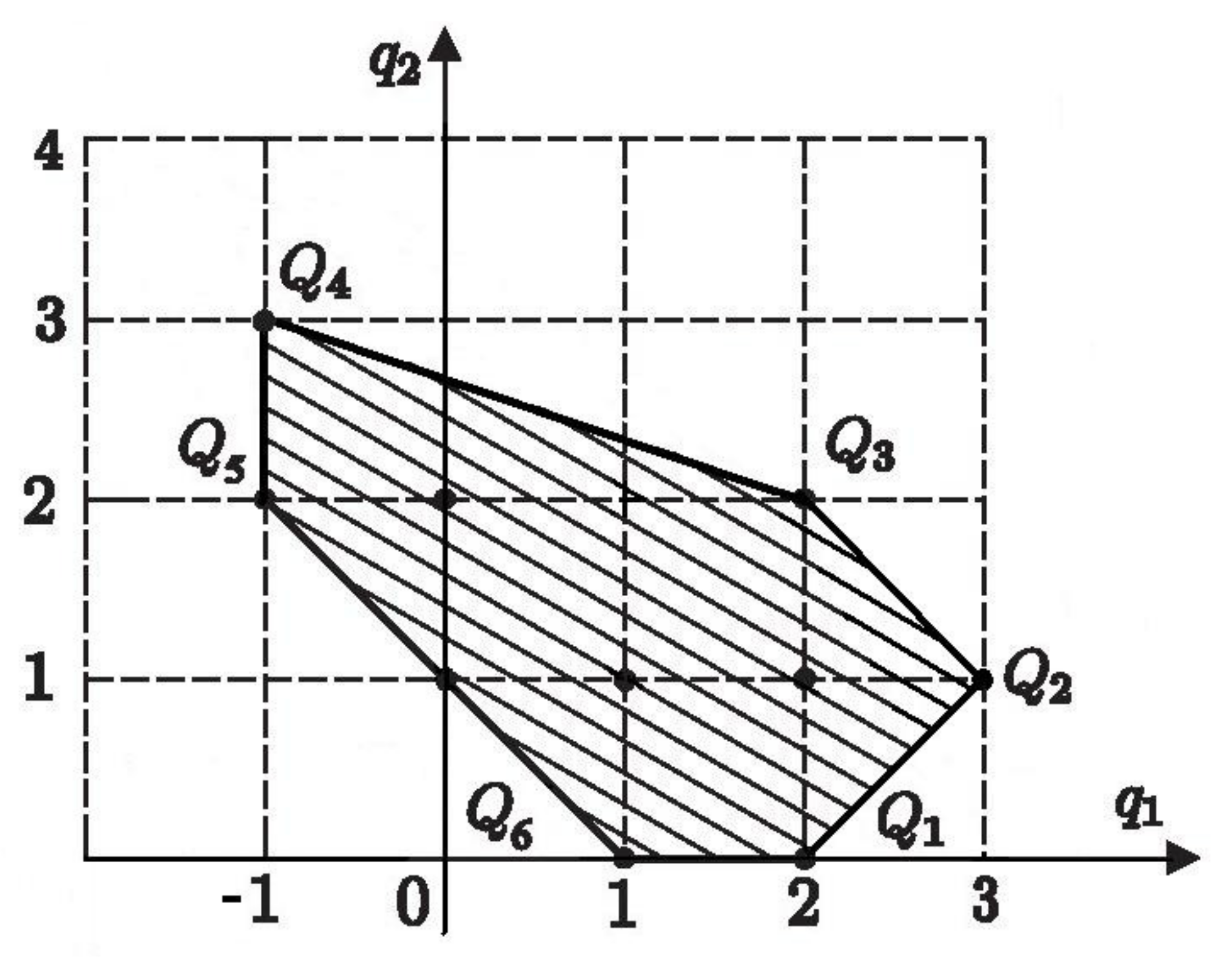
The Newton polygon of Equation (17) is given in Figure 1. The dominant balances near the point $x=\infty$ and their leading terms are

$$\begin{array}{c}(Q_1,Q_2):-\alpha y+\alpha x{y}^2=0,y\left(x\right)=1/x;\hfill \\ (Q_2,Q_3):-x{y}^2{y}_x=\alpha x{y}^2,y\left(x\right)=-\alpha x.\hfill \end{array}$$

(18)

Both provide Puiseux series near $x=\infty$ given by

$$y_1\left(x\right)=\sum _{k=0}^{+\infty }{a}_k{x}^{-1-k},y_2\left(x\right)=\sum _{k=0}^{+\infty }{b}_k{x}^{1-k},$$

(19)

where $a_0=1$, $b_0=-\alpha$, and the other constants $a_k$, and $k_k$ are uniquely determined for any $k\ge 1$.

Hence, from Theorem 7, we obtain

$$f(x,y)={\left\{\mu \left(x\right)\prod _{j=1}^2\{y-y_j\left(x\right)\}\right\}}_{+},$$

(20)

Note that the degree of f in the variable y is two.

Next, we study Puiseux solutions $x=x\left(y\right)$. Interchanging the variables $x\leftrightarrow y$ system (2) has the associated differential equation

$$\begin{array}{c}\hfill \alpha y(xy-1)x_y=1-x{y}^2.\end{array}$$

(21)

Finding the Newton polygon, the dominant balances related to the point $y=\infty$ and their leading terms are

$$\begin{array}{c}\alpha x{y}^2{x}_y=-\alpha x{y}^2,x\left(y\right)=-y/\alpha ;\hfill \\ \alpha x{y}^2-\alpha y=0,x\left(y\right)=1/y.\hfill \end{array}$$

(22)

These two balances have the associated Puiseux series

$$x_1\left(y\right)=\sum _{k=0}^{+\infty }{a}_k{y}^{1-k},x_j\left(y\right)=\sum _{k=0}^{+\infty }{b}_k{y}^{-1-k},$$

where $a_0=-1/\alpha$ and $b_0=1$ and the other constants $a_k$ and $b_k$ being uniquely determined for any $k\ge 1$. Therefore, in view of Theorem 7, we obtain

$$f(x,y)={\left\{\nu \left(y\right)\prod _{j=1}^2\{x-x_j\left(y\right)\}\right\}}_{+}.$$

(23)

Note that the degree of f in the variable x is two. Hence, it follows from (20) and (23) that the degree of $f(x,y)$ is two in both variables x and y. Therefore, we have

$$f(x,y)=f_0\left(x\right)+f_1\left(x\right)y+f_2\left(x\right)y^2,$$

(24)

where $f_i\left(x\right)$ are at most of degree two. Imposing that $f(x,y)$ is an invariant algebraic curve of system (2), we find that the unique invariant algebraic curve is $y=0$. This completes the proof of statement (b) and (c) for system (2).

In order to prove that system (2) is not Liouville integrable we must to see that it does not admit neither inverse integrating factor of the form $exp\left(g\right(x,y\left)\right)$ nor with $exp(g(x,y)/y^k)$, where $g(x,y)$ a polynomial of arbitrary degree m.

In the first case, g must satisfy

$$\begin{array}{c}\hfill (1-x{y}^2){\displaystyle \frac{\partial g}{\partial x}}+\left(\alpha y(xy-1)\right){\displaystyle \frac{\partial g}{\partial y}}=\mathrm{div}\mathcal{X}\end{array}$$

(25)

where $\mathcal{X}$ is the vector field associated with system (2) and its divergence is $\mathrm{div}\mathcal{X}=-y^2+\alpha xy+\alpha (xy-1)$. Expanding the polynomial $g(x,y)$ in its homogeneous parts as $g(x,y)={\sum }_{i=0}^n{g}_i(x,y)$, where $g_i$ is homogeneous polynomials in $(x,y),n\ge 1$ and $g_n\ne 0$. The homogeneous part $g_n$ for $n\ge 4$ must satisfy a differential equation whose solution is $g_n=d_n{(y+\alpha x)}^n$, where $d_n\ne 0$. The homogeneous part $g_{n-1}$ must satisfy a differential equation whose solution is $g_{n-1}=d_{n-1}{(y+\alpha x)}^{n-1},$ where $d_{n-1}$ is an arbitrary constant. Moreover, the homogeneous part $g_{n-2}$ must satisfy a differential equation whose solution is

$$g_{n-2}={\displaystyle \frac{d_{n}n\alpha {(y+x\alpha )}^{n}log(-x/y)}{{(y+x\alpha )}^2}}+G_{n-2}(y+x\alpha ),$$

where $G_{n-2}$ is an arbitrary function of $y+x\alpha$. Since $g_{n-2}$ must be a polynomial of degree $n-2$, then n must be zero, which is impossible. This means that g has at most degree 1, i.e., $g=d_0+d_{1}x+d_{2}y$, where $d_i\in \mathbb{C}$. Solving Equation (25), we find a contradiction.

In the second case we have $V=exp(g(x,y)/y^k)$ that satisfies

$$\begin{array}{c}\hfill (1-x{y}^2){\displaystyle \frac{\partial V}{\partial x}}+\left(\alpha y(xy-1)\right){\displaystyle \frac{\partial V}{\partial y}}=\mathrm{div}\left(X\right)V.\end{array}$$

(26)

Taking, as before, $g(x,y)$ as a polynomial of degree n, we have that if $k>4+n$, then Equation (26) cannot be satisfied. For $k=n+4$, the $g_n$ cannot be a homogeneous polynomial. For $k=n+3,n+2,n+1$, $g_n$ cannot be of degree n. For $k=n$, $g_{n-1}$ cannot be of degree $n-1$. Finally, for $k\le n-1$ then $g_{n-2}$ cannot be a homogeneous polynomial. Therefore, we have proved statement (d) for system (2).

The necessary conditions to have Puiseux integrability were given in [1]. Now we verify if system (2) is Puiseux integrable.

The form of the cofactor of any elementary curve $y-y_i\left(x\right)=0$ was given in [30]. The cofactor of any elementary solution $y=y_i\left(x\right)$, where $y_i\left(x\right)$ is any of the Puiseux series given in (19) can be computed using the equation

$$\mathcal{X}(y-y_i)=K_i(x,y)(y-y_i)$$

(27)

See, for instance, ref. [1,30]. By solving Equation (27), the cofactors are given by

$$K_i(x,y)=k_1^{\left(i\right)}\left(x\right)y+k_0^{\left(i\right)}\left(x\right),i=1,2.$$

because system (2) is of degree 2 in the variable y and where

$$\begin{array}{cc}\hfill k_1^{\left(i\right)}\left(x\right)=& x\alpha +x{y}_i^{\prime }\left(x\right),\hfill \\ \hfill k_0^{\left(i\right)}\left(x\right)=& -\alpha +x\alpha y\left(x\right)+xy\left(x\right)y_i^{\prime }\left(x\right).\hfill \end{array}$$

We denote by $K_0(x,y)$ the cofactor of $h\left(x\right)$ in (14). Since Equation (27) for $h\left(x\right)$ is $h^{\prime }\left(x\right)\dot{x}=K_0(x,y)h\left(x\right)$, we have

$$K_0=\frac{h^{\prime }\left(x\right)(1-x{y}^2)}{h\left(x\right)}$$

Hence, if we consider Equation (15) that in this case is

$${\alpha }_0{K}_0(x,y)+{\alpha }_1{K}_1(x,y)+{\alpha }_2{K}_2(x,y)=\mathrm{div}\mathcal{X}.$$

(28)

and where the divergence is $\mathrm{div}\mathcal{X}=-y^2+2\alpha xy+\alpha$ which implies that ${\alpha }_0\ne 0$. Therefore, collecting the first coefficients at different powers of x and y in expression (28), we find ${\alpha }_0=1$ to cancel the terms in $y^2$ and

$$\begin{array}{cc}\hfill & {\alpha }_1{K}_1(x,y)+{\alpha }_2{K}_2(x,y)+{\alpha }_3{K}_3(x,y)-\mathrm{div}\mathcal{X}\hfill \\ \hfill & =\alpha +\frac{1+{\alpha }_1-{\alpha }_2}{x}+\frac{{\alpha }_2}{\alpha x^2}+\mathcal{O}\left(\frac{1}{x^3}\right)\hfill \\ \hfill & +y\left[\alpha ({\alpha }_2-2)x-\frac{{\alpha }_1+{\alpha }_2}{x}+\frac{2{\alpha }_2-{\alpha }_1}{\alpha x^2}+\mathcal{O}\left(\frac{1}{x^3}\right)\right]\hfill \end{array}$$

(29)

This implies that $\alpha =0$, which is not possible.

Finally, we take into account the existence of multiple Puiseux solutions which implies the existence of exponential factors. First, we study the existence of an exponential factor of the form $F=exp\left(g\right(x,y\left)\right)$ with a cofactor $K_4(x,y)=k_1^{\left(4\right)}\left(x\right)y+k_0^{\left(4\right)}\left(x\right)$. We substitute F into the equation

$$\begin{array}{c}\hfill (1-x{y}^2){\displaystyle \frac{\partial F}{\partial x}}+\left(\alpha y(xy-1)\right){\displaystyle \frac{\partial F}{\partial y}}=K_{i}F.\end{array}$$

(30)

proposing $g(x,y)$ as a polynomial of degree n in y, i.e.,

$$g(x,y)=\sum _{i=0}^n{g}_i\left(x\right)y^i,$$

(31)

with $n\ge 1$. From the higher powers in y of expression (30), we obtain $g_n\left(x\right)=c_n\ne 0$ and $g_{n-1}\left(x\right)=c_{n}n\alpha x+c_{n-1}$. The unique possibility that Equation (30) is compatible takes $n=1$ and $g_i\left(x\right)=0$ for $i=0,\dots ,n-2$ and in this case

$$k_1^{\left(4\right)}\left(x\right)=c_n\alpha ,k_0^{\left(4\right)}\left(x\right)=-c_n\alpha .$$

where we can take without lost of generality $c_n=1$. Moreover, using this new cofactor, $K_4=-\alpha +\alpha y$, the equation

$$\begin{array}{cc}\hfill & {\alpha }_1{K}_1(x,y)+{\alpha }_2{K}_2(x,y)+{\alpha }_3{K}_3(x,y)+{\alpha }_4{K}_4(x,y)=\mathrm{div}\mathcal{X}\hfill \end{array}$$

(32)

has no solution.

Second, we study the existence of exponential factors of the form $F=exp(g(x,y)/(y-y_i\left(x\right))$ for the two Puiseux series given in (19) with cofactor of the form

$$K_j(x,y)=k_1^{\left(j\right)}\left(x\right)y+k_0^{\left(j\right)}\left(x\right),$$

for $j=5,6$. We propose $g(x,y)$ as in (31) and by substituting into Equation (30) we obtain

$$\begin{array}{c}{g}_n\left(x\right)=c_n,g_{n-1}=c_{n}n\alpha x+c_{n-1},\\ {\displaystyle g_{n-2}=c_{n-1}(n-1)\alpha x+\frac{1}{2}{c}_n(n^2-n){\alpha }^2{x}^2-c_n\alpha nlogx+c_{n-2}.}\end{array}$$

Moreover, the unique possibility that Equation (30) be compatible is taking $n=2$ and $g_i\left(x\right)=0$ for $i=0,\dots ,n-3$ and in this case we have

$$\begin{array}{c}{k}_1^{\left(j\right)}\left(x\right)=-2c_n\alpha +c_{n-1}\alpha +x\alpha +2c_{n}x{\alpha }^2+x{y}_i^{\prime }\left(x\right),\\ k_0^{\left(j\right)}\left(x\right)=2c_n\alpha -x\alpha -c_{n-1}x\alpha -2c_n{x}^2{\alpha }^2+x^2\alpha y_i\left(x\right)+x^2{y}_i\left(x\right)y_i^{\prime }\left(x\right),\end{array}$$

where $y_i\left(x\right)$ are the Puiseux solutions given in (19). Finally, the equation

$$\sum _{i=1}^6{\alpha }_i{K}_i=\mathrm{div}\mathcal{X}$$

(33)

has no solution. In fact also implies $\alpha =0$ which is not possible. So, statement (e) for system (2) is proved. This concludes the proof of Theorem 1 for system (2).

5. Proof of Theorem 1 for System (4)

We recall a and b are positive parameters. In this case, system (4) has the unique finite singular point

$$P_1=\left(b,\frac{b}{a+b^2}\right).$$

The Jacobian matrix evaluated at the point $(1,1)$ has determinant $a+b^2$ and so the eigenvalues ${\lambda }_1$ and ${\lambda }_2$ satisfy ${\lambda }_1{\lambda }_2=a+b^2>0$. Therefore, ${\lambda }_1{\lambda }_2>0$ and it follows from Theorem 5 that system (4) has no a formal first integral around $P_1$ and so has no global $C^{\infty }$ first integrals implying that it also does not have global analytic first integrals. This concludes the proof of statement (a) for system (4). In particular, this means that system (4) has no polynomial first integrals.

To prove statement (b), we use the method proposed in [1]. First, we construct the associated differential equation of system (4) given by

$$\begin{array}{c}\hfill (-x+ay+x{y}^2)y_x=b-ay-x^{2}y\end{array}$$

(34)

The Newton polygon of Equation (34) has the following dominant balances near the point $x=\infty$ and corresponding leading terms

$$\begin{array}{c}(Q_1,Q_2):x^{2}y{y}_x+x^{2}y=0,y\left(x\right)=-x;\hfill \\ (Q_2,Q_3):b-x^{2}y=0,y\left(x\right)=b/x^2.\hfill \end{array}$$

(35)

Both provide Puiseux series near $x=\infty$ given by

$$y_1\left(x\right)=\sum _{k=0}^{+\infty }{a}_k{x}^{1-k},y_2\left(x\right)=\sum _{k=0}^{+\infty }{b}_k{x}^{-2-k},$$

(36)

where $a_0=-1$, $b_0=b$, and the other constants $a_k$, and $k_k$ are uniquely determined for any $k\ge 1$.

Hence, from Theorem 7, we obtain

$$f(x,y)={\left\{\mu \left(x\right)\prod _{j=1}^2\{y-y_j\left(x\right)\}\right\}}_{+},$$

(37)

Note that the degree of f in the variable y is two.

Next we study Puiseux solutions $x=x\left(y\right)$. Interchanging the variables $x\leftrightarrow y$ system (4) has the associated differential equation

$$\begin{array}{c}\hfill (b-ay-x^{2}y)x_y=-x+ay+x^{2}y.\end{array}$$

(38)

Finding the Newton polygon, the dominant balances related to the point $y=\infty$ and their leading terms are

$$\begin{array}{c}-x^{2}y{x}_y=x^{2}y,x\left(y\right)=-y;\hfill \\ (b-x^{2}y)x_y=0,x\left(y\right)=b_0,\hfill \end{array}$$

(39)

where $b_0=\pm i\sqrt{a}$. These two balances have the associated Puiseux series

$$x_1\left(y\right)=\sum _{k=0}^{+\infty }{a}_k{y}^{1-k},x_j\left(y\right)=\sum _{k=0}^{+\infty }{b}_k{y}^{-k},$$

(40)

where $a_0=-1$ and $b_0=\pm i\sqrt{a}$ and the other constants $a_k$ and $b_k$ being uniquely determined for any $k\ge 1$. Therefore, in view of Theorem 7, we obtain

$$f(x,y)={\left\{\nu \left(y\right)\prod _{j=1}^3\{x-x_j\left(y\right)\}\right\}}_{+}.$$

(41)

Note that the degree of f in the variable x is three. Hence, it follows from (37) and (41) that the degree of $f(x,y)$ is two in the variable y and three in x. Therefore, we have $f(x,y)$ takes the form (24) where $f_i\left(x\right)$ are at most of degree three. Imposing that such a curve is an invariant algebraic curve of system (4), we obtain a contradiction and therefore it does not exist. This completes the proof of statements (b) and (c) for system (4).

System (4) is only Liouville integrable if it admits an inverse integrating factor of the form $exp\left(g\right(x,y\left)\right)$, where $g(x,y)$ is a polynomial of arbitrary degree m.

Therefore, g must satisfy

$$\begin{array}{c}\hfill (-x+ay+x{y}^2){\displaystyle \frac{\partial g}{\partial x}}+(b-ay-x{y}^2){\displaystyle \frac{\partial g}{\partial y}}=\mathrm{div}\mathcal{X}\end{array}$$

(42)

where $\mathrm{div}\mathcal{X}=-1-a-2xy+y^2$. Expanding the polynomial $g(x,y)$ in its homogeneous parts as $g(x,y)={\sum }_{i=0}^n{g}_i(x,y)$, where $g_i$ are homogeneous polynomials in $(x,y),n\ge 1$ and $g_n\ne 0$. The homogeneous part $g_n$ for $n\ge 4$ must satisfy a differential equation whose solution is $g_n=d_n{(x+y)}^n$ where $d_n\ne 0$. The homogeneous part $g_{n-1}$ must satisfy a differential equation whose solution is $g_{n-1}=d_{n-1}{(x+y)}^{n-1},$ where $d_{n-1}$ is an arbitrary constant. Moreover, the homogeneous part $g_{n-2}$ must satisfy a differential equation whose solution is

$$g_{n-2}={\displaystyle \frac{d_{n}n{(x+y)}^{n-1}}{y}}+G_{n-2}(x+y),$$

where $G_{n-2}$ is an arbitrary function of $x+y$. Since $g_{n-2}$ must be a polynomial of degree $n-2$ then n must be zero, which is impossible. This means that g has at most degree 1 i.e., $g=d_0+d_{1}x+d_{2}y$ where $d_i\in \mathbb{C}$. Solving Equation (42) for such g we get a contradiction. Therefore we have proved statement (d) for system (2).

Next we verify if system (4) is Puiseux integrable.

Solving Equation (27) for system (4) the cofactors are given by

$$K_i(x,y)=k_0^{\left(i\right)}\left(x\right)=-(a+x^2)(1-y_i^{\prime }\left(x\right)).$$

The cofactor $K_0(x,y)$ of $h\left(x\right)$ in (14) is

$$K_0=\frac{h^{\prime }\left(x\right)(-x+ay+x{y}^2)}{h\left(x\right)}$$

Therefore, if we consider the Equation (15), collecting the first coefficients at different powers of x and y in expression (28), we get

$$\begin{array}{cc}\hfill & {\alpha }_0{K}_0(x,y)+{\alpha }_1{K}_1(x,y)+{\alpha }_2{K}_2(x,y)-\mathrm{div}\mathcal{X}\hfill \\ \hfill & =({\alpha }_0-2)x+\frac{a{\alpha }_0}{x}+\mathcal{O}\left(\frac{1}{x^4}\right)\hfill \\ \hfill & +y\left[-{\alpha }_0+\frac{3b}{x}+\frac{2}{x^2}-\frac{(21+4a)b}{2x^3}+\mathcal{O}\left(\frac{1}{x^4}\right)\right]\hfill \end{array}$$

(43)

This implies $a=b=0$ which is not possible.

Now we study the existence of multiple Puiseux solutions with their corresponding exponential factors. First, we study if the infinity curve is multiple, i.e., the existence of an exponential factor of the form $F=exp\left(g\right(x,y\left)\right)$ with a cofactor $K_4(x,y)=k_1^{\left(4\right)}\left(x\right)y+k_0^{\left(4\right)}\left(x\right)$. We substitute F into the equation

$$\begin{array}{c}\hfill (-x+ay+x^{2}y){\displaystyle \frac{\partial F}{\partial x}}+(b-ay-x^{2}y){\displaystyle \frac{\partial F}{\partial y}}=K_{i}F.\end{array}$$

(44)

proposing $g(x,y)$ as a polynomial of degree n in y, i.e.

$$g(x,y)=\sum _{i=0}^n{g}_i\left(x\right)y^i,$$

(45)

with $n\ge 1$. From the higher power in y of expression (44), we obtain $g_n\left(x\right)=c_n\ne 0$ and $g_{n-1}\left(x\right)=c_{n}nx+c_{n-1}$. The unique value for n that Equation (44) is compatible is for $n=2$ and $g_i\left(x\right)=0$ for $i=0,\dots ,n-2$ and in this case

$$\begin{array}{cc}\hfill k_1^{\left(4\right)}\left(x\right)& =-2b{c}_n+a{c}_{n-1}+2(1+a)c_{n}x+c_{n-1}{x}^2+2c_n{x}^3,\hfill \\ \hfill k_0^{\left(4\right)}\left(x\right)& =-b{c}_{n-1}-2b{c}_{n}x.\hfill \end{array}$$

where we can take $c_n=1$. However, using this cofactor $K_4$ the equation

$$\begin{array}{cc}\hfill & {\alpha }_1{K}_1(x,y)+{\alpha }_2{K}_2(x,y)+{\alpha }_3{K}_3(x,y)+{\alpha }_4{K}_4(x,y)=\mathrm{div}\mathcal{X}\hfill \end{array}$$

(46)

has no solution for any ${\alpha }_i$.

Second we study the existence of exponential factors of the form $F=exp(g(x,y)/(y-y_i\left(x\right))$ for the two Puiseux series given in (36) with a cofactor of the form

$$K_j(x,y)=k_1^{\left(j\right)}\left(x\right)y+k_0^{\left(j\right)}\left(x\right),$$

for $j=5,6$. We propose $g(x,y)$ as in (45) and by substituting into Equation (44) we have

$$g_n\left(x\right)=c_n,g_{n-1}=n{c}_{n}x+c_{n-1}.$$

Moreover, the unique possibility that Equation (44) is compatible takes $n=2$ and $g_i\left(x\right)=0$ for $i=0,\dots ,n-2$ and in this case we have

$$\begin{array}{c}{k}_1^{\left(j\right)}\left(x\right)=-2b{c}_n+a{c}_{n-1}+2c_{n}x+2a{c}_{n}x+c_{n-1}{x}^2+2c_n{x}^3,\\ k_0^{\left(j\right)}\left(x\right)=-a-b{c}_{n-1}-2b{c}_{n}x-x^2-a{y}_i^{\prime }\left(x\right)-x^2{y}_i^{\prime }\left(x\right),\end{array}$$

where $y_i\left(x\right)$ are the Puiseux solutions given in (36). Finally the Equation (33) for this case has no solution. Therefore statement (e) for system (4) is proved. This concludes the proof of Theorem 1 for system (4).

6. Proof of Theorem 1 for System (6)

System (6) has the unique finite singular point $(A,B/A)$ with $A\ne 0$. The eigenvalues of this singular point satisfy that ${\lambda }_1{\lambda }_2=A\ne 0$. If $A>0$ then ${\lambda }_1{\lambda }_2>0$ and it follows from Theorem 5 that system (2) has no a formal first integral around $(A,B/A)$ and so has no global $C^{\infty }$ first integrals implying that it also does not have global analytic first integrals. If $A<0$ then ${\lambda }_1+{\lambda }_2=B-1-A^2$. If $B-1-A^2\ne 0$ then, again from Theorem 5, system (2) has no a formal first integral around the singular point $(A,B/A)$ and so has no global $C^{\infty }$ first integrals implying that it also does not have global analytic first integrals nor polynomial. In the case $B=1+A^2$, the system has a weak focus at the singular point $(A,B/A)$ and we arrive to the same conclusion because a weak focus does not even have a continuous first integral around it. This proof of statement (a) for system (6).

Now we prove statement (b). The associated differential equation to system (6) is

$$\begin{array}{c}\hfill (A+x^{2}y-Bx-x)y_x=Bx-x^{2}y.\end{array}$$

(47)

The dominant balances near the point $x=\infty$ and their leading terms are

$$\begin{array}{c}(Q_1,Q_2):x^{2}y{y}_x+x^{2}y=0,y\left(x\right)=-x;\hfill \\ (Q_2,Q_3):Bx-x^{2}y=0,y\left(x\right)=B/x.\hfill \end{array}$$

(48)

Both provide Puiseux series near $x=\infty$ given by

$$y_1\left(x\right)=\sum _{k=0}^{+\infty }{a}_k{x}^{1-k},y_2\left(x\right)=\sum _{k=0}^{+\infty }{b}_k{x}^{-1-k},$$

(49)

where $a_0=-1$, $b_0=B$, and the other constants $a_k$, and $k_k$ are uniquely determined for any $k\ge 1$. Therefore, by Theorem 7, we obtain

$$f(x,y)={\left\{\mu \left(x\right)\prod _{j=1}^2\{y-y_j\left(x\right)\}\right\}}_{+},$$

(50)

Then, the degree of f in the variable y is two.

Now, we interchange the variables $x\leftrightarrow y$ in system (6) the associated differential equation is now

$$\begin{array}{c}\hfill (Bx-x^{2}y)x_y=A+x^{2}y-Bx-x.\end{array}$$

(51)

Finding the Newton polygon, the dominant balances related to the point $y=\infty$ and their leading terms are

$$\begin{array}{c}-x^{2}y{x}_y=x^{2}y,x\left(y\right)=-y;\hfill \\ A+x^{2}y=0,x\left(y\right)=b_0/y^{1/2},\hfill \end{array}$$

(52)

where $b_0=\pm i\sqrt{A}$. These two balances have the associated Puiseux series

$$x_1\left(y\right)=\sum _{k=0}^{+\infty }{a}_k{y}^{1-k},x_j\left(y\right)=\sum _{k=0}^{+\infty }{b}_k{y}^{-1/2-k},$$

(53)

where $a_0=-1$ and $b_0=\pm i\sqrt{A}$ and the other constants $a_k$ and $b_k$ being uniquely determined for any $k\ge 1$. Therefore, in view of Theorem 7, we obtain

$$f(x,y)={\left\{\nu \left(y\right)\prod _{j=1}^3\{x-x_j\left(y\right)\}\right\}}_{+}.$$

(54)

Note that the degree of f in the variable x is three. Hence, it follows from (50) and (54) that the degree of $f(x,y)$ is two in variable y and three in x. Therefore, we have that $f(x,y)$ is of the form (24), where $f_i\left(x\right)$ is at most of degree three. Imposing that such a curve $f(x,y)=0$ exists for system (4), we find a contradiction. This completes the proof of statements (b) and (c) for system (6).

To verify if system (6) is Liouville integrable only remains to check if admits an inverse integrating factor of the form $exp\left(g\right(x,y\left)\right)$, where $g(x,y)$ is a polynomial of arbitrary degree m. Hence, g must satisfy

$$\begin{array}{c}\hfill (A+x^{2}y-Bx-x){\displaystyle \frac{\partial g}{\partial x}}+(Bx-x^{2}y){\displaystyle \frac{\partial g}{\partial y}}=\mathrm{div}\mathcal{X}\end{array}$$

(55)

with $\mathrm{div}\mathcal{X}=-1-B-x^2+2xy$. We write the polynomial $g(x,y)$ of degree n in its expansion in homogeneous polynomials $g_i(x,y)$ with $n\ge 1$ and $g_n\ne 0$. The homogeneous part $g_n$ for $n\ge 4$ must satisfy a differential equation whose solution is $g_n=d_n{(x+y)}^n$ where $d_n\ne 0$. The differential equation of the homogeneous part $g_{n-1}$ has the solution $g_{n-1}=d_{n-1}{(x+y)}^{n-1},$ where $d_{n-1}$ is an arbitrary constant. Moreover, the homogeneous part $g_{n-2}$ must satisfy a differential equation whose solution is

$$g_{n-2}=d_{n}n{(x+y)}^{n-2}log\left(\frac{x}{y}\right)+G_{n-2}(x+y),$$

where $G_{n-2}$ is an arbitrary function of $x+y$. Since $g_{n-2}$ must be a polynomial of degree $n-2$ then n must be zero, which is impossible. This means that g has at most degree 1 i.e., $g(x,y)=d_0+d_{1}x+d_{2}y$ where $d_i\in \mathbb{C}$. Solving Equation (55) for such g we get a contradiction. Therefore, we have proved statement (d) for system (6).

Finally, we study if system (6) is Puiseux integrable.

Solving Equation (27) for system (6) the cofactors are given by $K_i(x,y)=k_0^{\left(i\right)}\left(x\right)=-x^2-x^2{y}_i^{\prime }\left(x\right))$. The cofactor $K_0(x,y)$ of $h\left(x\right)$ in (14) is

$$K_0=\frac{h^{\prime }\left(x\right)(A+x^{2}y-Bx-x)}{h\left(x\right)}$$

If we consider the Equation (15), the first coefficients at different powers of x and y in expression (28) are given by

$$\begin{array}{cc}\hfill & {\alpha }_0{K}_0(x,y)+{\alpha }_1{K}_1(x,y)+{\alpha }_2{K}_2(x,y)-\mathrm{div}\mathcal{X}\hfill \\ \hfill & =y\left[(-2+{\alpha }_0)x+\mathcal{O}\left(\frac{1}{x^2}\right)\right]\hfill \\ \hfill & +(1+2B-{\alpha }_0-B{\alpha }_0-{\alpha }_1)+\frac{A({\alpha }_0+{\alpha }_1)}{x}+\mathcal{O}\left(\frac{1}{x^2}\right),\hfill \end{array}$$

(56)

which implies $A=B=0$, which is not possible.

Now we study the existence of exponential factors associated with multiple Puiseux solutions. First, we study the existence of an exponential factor of the form $F=exp\left(g\right(x,y\left)\right)$ with a cofactor $K_4(x,y)=k_1^{\left(4\right)}\left(x\right)y+k_0^{\left(4\right)}\left(x\right)$. We substitute F into the equation

$$\begin{array}{c}\hfill (A+x^{2}y-Bx-x){\displaystyle \frac{\partial F}{\partial x}}+(Bx-x^{2}y){\displaystyle \frac{\partial F}{\partial y}}=K_{i}F.\end{array}$$

(57)

proposing $g(x,y)$ as a polynomial of degree n in y, with $n\ge 1$. From the higher power in y of expression (57), we obtain $g_n\left(x\right)=c_n\ne 0$ and $g_{n-1}\left(x\right)=c_{n}nx+c_{n-1}$. The unique value for n that Equation (57) is compatible is for $n=2$ and $g_i\left(x\right)=0$ for $i=0,\dots ,n-2$ and in this case

$$\begin{array}{cc}\hfill k_1^{\left(4\right)}\left(x\right)& =-2A{c}_n+2c_{n}x+c_{n-1}{x}^2+2c_n{x}^3,\hfill \\ \hfill k_0^{\left(4\right)}\left(x\right)& =-B{c}_{n-1}x-2B{c}_n{x}^2.\hfill \end{array}$$

where we can take $c_n=1$. However, using this cofactor $K_4$ Equation (46) for such a case has no solution for any values of ${\alpha }_i$.

Next, we study the existence of exponential factors of the form $F=exp(g(x,y)/(y-y_i\left(x\right))$ for the two Puiseux series given in (49) with cofactor of the form $K_j(x,y)=k_1^{\left(j\right)}\left(x\right)y+k_0^{\left(j\right)}\left(x\right)$, for $j=5,6$. We propose $g(x,y)$ as in (45) and substituting into Equation (57) obtaining

$$g_n\left(x\right)=c_n,g_{n-1}=n{c}_{n}x+c_{n-1}.$$

Moreover, the unique possibility that Equation (57) is compatible takes $n=2$ and $g_i\left(x\right)=0$ for $i=0,\dots ,n-2$ and in this case we have

$$\begin{array}{c}{k}_1^{\left(j\right)}\left(x\right)=-2A{c}_n+2c_{n}x+c_{n-1}{x}^2+2c_n{x}^3,\\ k_0^{\left(j\right)}\left(x\right)=-x(B{c}_{n-1}+x+2B{c}_{n}x+x{y}_i^{\prime }\left(x\right)),\end{array}$$

where $y_i\left(x\right)$ are the Puiseux solutions given in (53). Finally, the Equation (33) for this case has no solution. Therefore, statement (e) for system (6) is proved and this completes the proof of Theorem 1 for system (6).

7. Conclusions

A complete algebraic characterization of the first integrals of the Higgins–Selkov, Selkov and Brusellator oscillators is given here. First, the study focus on the study of the invariant algebraic curves of such systems. The unique system that has invariant algebraic curve is the Selkov oscillator which has the invariant curve $y=0$. Next, it is proved that such systems are not Darboux, Liouvillian nor Puiseux integrable. In order to determine the Puiseux integrability of such systems, the multiple Puiseux solutions are also studied. The nonexistence of centers for such oscillators is also proved.

References

- Demina, M.; Giné, J.; Valls, C. Puiseux integrability of differential equations. Qual. Theory Dyn. Syst. 2022, 21, 1–35. [Google Scholar] [CrossRef]
- Giné, J.; Grau, M. Weierstrass integrability of differential equations. Appl. Math. Lett. 2010, 23, 523–526. [Google Scholar] [CrossRef] [Green Version]
- Giné, J.; Llibre, J. Formal Weierstrass nonintegrability criterion for some classes of polynomial differential systems in C2. Int. J. Bifurc. Chaos 2020, 30, 2050064. [Google Scholar] [CrossRef]
- Giné, J.; Llibre, J. Strongly formal Weierstrass non-integrability for polynomial differential systems in C2. Electron. J. Qual. Theory Differ. Equ. 2020, 2020, 1–16. [Google Scholar] [CrossRef]
- Llibre, J.; Valls, C. Weierstrass integrability of complex differential equations. Acta Math. Sin. Engl. Ser. 2021, 37, 1497–1506. [Google Scholar] [CrossRef]
- Giné, J.; Valls, C. The Liouvillian integrability of several oscillators. Int. J. Bifurc. Chaos 2019, 29, 1950069. [Google Scholar] [CrossRef]
- Demina, M.V. From Puiseux series to invariant algebraic curves: The FitzHugh-Nagumo model. arXiv 2018, arXiv:1804.02542. [Google Scholar]
- Demina, M.V. Invariant algebraic curves for Liénard dynamical systems revisited. Appl. Math. Lett. 2018, 84, 42–48. [Google Scholar] [CrossRef] [Green Version]
- Demina, M.V. Novel algebraic aspects of Liouvillian integrability for two-dimensional polynomial dynamical systems. Phys. Lett. A 2018, 382, 1353–1360. [Google Scholar] [CrossRef]
- Demina, M.V.; Valls, C. On the Poincaré problem and Liouvillian integrability of quadratic Liénard differential equations. Proc. R. Soc. Edinb. Sect. A 2020, 150, 3231–3251. [Google Scholar] [CrossRef]
- Ferčec, B.; Giné, J. Formal Weierstrass integrability for a Linard differential system. J. Math. Anal. Appl. 2021, 499, 125016. [Google Scholar] [CrossRef]
- Giné, J.; Llibre, J. A new sufficient condition in order that the real Jacobian conjecture in R2 holds. J. Differ. Equ. 2021, 281, 333–340. [Google Scholar] [CrossRef]
- Algaba, A.; Checa, I.; Gamero, E.; García, C. Characterizing orbital-reversibility through normal forms. Qual. Theory Dyn. Syst. 2021, 20, 1–37. [Google Scholar] [CrossRef]
- Algaba, A.; Gamero, E.; García, C. Orbital Hypernormal Forms. Symmetry 2021, 13, 1500. [Google Scholar] [CrossRef]
- Giné, J.; Maza, S. The reversibility and the center problem. Nonlinear Anal. 2011, 74, 695–704. [Google Scholar] [CrossRef]
- Higgins, J. A chemical mechanism for oscillation of glycolytic intermediates in yeast cells. Proc. Natl. Acad. Sci. USA 1964, 51, 989–994. [Google Scholar] [CrossRef] [Green Version]
- Knoke, B.; Marhl, M.; Perc, M.; Schuster, S. Equality of average and steady-state levels in some nonlinear models of biological oscillations. Theory Biosci. 2008, 127, 1–14. [Google Scholar] [CrossRef]
- Artés, J.C.; Llibre, J.; Valls, C. Dynamics of the Higgins–Selkov and Selkov systems. Chaos Solitons Fractals 2018, 114, 145–150. [Google Scholar] [CrossRef] [Green Version]
- Sel’kov, E.E. Self-Oscillations in Glycolysis. Eur. J. Biochem. 1968, 4, 79–86. [Google Scholar] [CrossRef]
- Lotka, A.J. Contribution to the Theory of Periodic Reactions. J. Phys. Chem. 1910, 14, 271–274. [Google Scholar] [CrossRef] [Green Version]
- Strogatz, S.H. Nonlinear Dynamics and Chaos with Student Solutions Manual: With Applications to Physics, Biology, Chemistry, and Engineering.; CRC Press: Boca Raton, MA, USA, 2018; p. 207. [Google Scholar]
- Giné, J.; Santallusia, X. Implementation of a new algorithm of computation of the Poincaré-Liapunov constants. J. Comput. Appl. Math. 2004, 166, 465–476. [Google Scholar] [CrossRef] [Green Version]
- Dumortier, F.; Llibre, J.; Artés, J.C. Qualitative Theory of Planar Differential Systems; Springer: New York, NY, USA, 2006. [Google Scholar]
- Zhang, X. Liouvillian integrability of polynomial differential systems. Trans. Am. Math. Soc. 2016, 368, 607–620. [Google Scholar] [CrossRef] [Green Version]
- Zhang, X. Integrability of Dynamical Systems: Algebra and Analysis; Developments in Mathematics, 47; Springer: Singapore, 2017. [Google Scholar]
- Singer, M.F. Liouvillian first integrals of differential equations. Trans. Am. Math. Soc. 1992, 333, 673–688. [Google Scholar] [CrossRef]
- Christopher, C.J. Liouvillian first integrals of second order polynomial differential equations. Electron. J. Differ. Equ. 1999, 49, 1–7. [Google Scholar]
- Poincaré, H. Mémoire sur les courbes définies par les équations différentielles. In Oeuvres de Henri Poincaré, Volume I; Gauthier–Villars: Paris, France, 1951; pp. 95–114. [Google Scholar]
- Li, W.; Llibre, J.; Zhang, X. On the differentiability of first integrals of two dimensional flows. Proc. Am. Math. Soc. 2002, 130, 2079–2088. [Google Scholar] [CrossRef]
- García, I.A.; Giacomini, H.; Giné, J. Generalized nonlinear superposition principles for polynomial planar vector fields. J. Lie Theory 2005, 15, 89–104. [Google Scholar]
Figure 1.
The Newton polygon of Equation (17).
Publisher’s Note: MDPI stays neutral with regard to jurisdictional claims in published maps and institutional affiliations. |
© 2022 by the author. Licensee MDPI, Basel, Switzerland. This article is an open access article distributed under the terms and conditions of the Creative Commons Attribution (CC BY) license (https://creativecommons.org/licenses/by/4.0/).
Share and Cite
MDPI and ACS Style
Giné, J. On the Dynamics of Higgins–Selkov, Selkov and Brusellator Oscillators. Symmetry 2022, 14, 438. https://0-doi-org.brum.beds.ac.uk/10.3390/sym14030438
AMA Style
Giné J. On the Dynamics of Higgins–Selkov, Selkov and Brusellator Oscillators. Symmetry. 2022; 14(3):438. https://0-doi-org.brum.beds.ac.uk/10.3390/sym14030438
Chicago/Turabian StyleGiné, Jaume. 2022. "On the Dynamics of Higgins–Selkov, Selkov and Brusellator Oscillators" Symmetry 14, no. 3: 438. https://0-doi-org.brum.beds.ac.uk/10.3390/sym14030438
Note that from the first issue of 2016, this journal uses article numbers instead of page numbers. See further details here.