Nonlinear Transformation of Sine Wave within the Framework of Symmetric (2+4) KdV Equation

Abstract

This paper considers the transformation of a sine wave in the framework of the extended modified Korteweg–de Vries equation or (2+4) KdV, which includes a combination of cubic and quintic nonlinearities. It describes the internal waves in a medium with symmetric vertical density stratification, and all the considerations in this study are produced for the reasonable combinations of the signs of the coefficients for nonlinear and dispersive terms, provided by this physical problem. The features of Riemann waves—solutions of the dispersionless limit of the model—are described in detail: The times and levels of breaking are derived in an implicit analytic form depending on the amplitude of the initial sine wave. It is demonstrated that the shock occurs at two (for small amplitudes) or four (for moderate and large amplitudes) levels per period of sine wave. Breaking at different levels occurs at different times. The symmetric (2+4) KdV equation is not integrable, but nevertheless it has stationary solutions in the form of traveling solitary waves of both polarities with a limiting amplitude. With the help of numerical calculations, the features of the processes of a sinusoidal wave evolution and formation of undular bores are demonstrated and analyzed. Qualitative features of multiple inelastic interactions of emerging soliton-like pulses are displayed.

1. Introduction

Nonlinear partial differential equations of evolutionary type often arise as an approximate mathematical formulation for complex nonlinear physical phenomena. The equations of the Korteweg–de Vries (KdV) family describe nonlinear wave effects in a number of physical contexts: in hydrodynamics (shallow water waves and internal waves in stratified basins) [1,2,3], plasma physics [4,5,6], quantum fluid dynamics [7], and some others [8,9,10,11]; they appear in many areas of applied sciences and engineering. Exact travelling wave solutions of such nonlinear evolution equations can perform a significant part in the understanding of different physical processes because they describe various phenomena in nature.

Energy cascades from long to short waves are inherent in many physical systems, and here it is important to understand the features and details of the disintegration of long disturbances, alongside their steepening and decomposition into solitary waves and small-scale dispersive trains of linear waves. KdV-type equations also serve as generic mathematical models for the description of undular bores’ formation, when the effects of higher-order nonlinearity become important [12,13]. In fact, solitons and undular bores appear as intermediate asymptotics in all models describing a nonlinear process of long wave disintegration in a weakly dispersive medium [14,15].

This paper considers an extended modified Korteweg–de Vries equation ((2+4) KdV) containing a combination of third- and fifth-degree nonlinear terms in the same order of smallness:

$$\frac{\partial \zeta }{\partial t}+{\mathsf{\alpha }}_1{\zeta }^2\frac{\partial \zeta }{\partial x}+{\mathsf{\alpha }}_3{\zeta }^4\frac{\partial \zeta }{\partial x}+\mathsf{\beta }\frac{{\partial }^3\zeta }{\partial x^3}=0,$$

(1)

where alpha and beta are constants determined in the physical context. This equation improves the description of wave dynamics near the point of zero cubic nonlinearity due to the fifth-degree nonlinearity, and such a generalization naturally highlights a variety of qualitatively new phenomena in the dynamics of localized, solitonic (nonradiating) waves. Equation (1) is an analogue of the Gardner equation [12,13], which is valid for describing situations with a change in the sign of the quadratic nonlinearity coefficient. Equation (1), also called the (2+4) KdV equation, was particularly derived for mode I waves at interfaces in a three-layer fluid flow symmetric with respect to half-depth [16,17]. Nonlinearity and dispersion coefficients are determined by a specific physical situation and depend on the parameters of the medium in which the waves propagate.

It should be noted that, from a purely mathematical point of view, Equation (1) can have “parasitic” solutions corresponding to the case of large nonlinear corrections. For example, if the quintic nonlinearity term prevails, then field self-focusing is possible with the formation of singularities [8,18]. Such effects, however, are nonphysical and are far beyond the application of the considered equation in the context of weakly nonlinear internal waves in a three-layer fluid.

Within the framework of Equation (1), we will consider the process of transformation of a long sinusoidal wave. This transformation includes the stages of (i) steepening, (ii) the formation of short-period solitary waves, and (iii) their further multiple interactions.

The process of steepening or nonlinear wave deformation, when the dispersion effects are still vanishingly small, can be analytically described in terms of Riemann waves, and this approach is classical (see, for example, Whitham (1974)) but it was usually considered in the case of weak (quadratic and cubic) nonlinearities [19,20]. Equation (1) provides us with a context for studying wave steepening in a highly nonlinear case.

The dynamics of soliton ensembles are often studied in the context of the “soliton gas” or “soliton turbulence” [21,22]. These phenomena can also be of interest within the framework of Equation (1), since it admits various regimes of solitonic interactions, including those of different polarities; moreover, they are inelastic. The property of inelasticity of solitonic interactions was stated for generalized KdV-type equations [23,24].

The main goal of this study is to analyze the process of the transformation of long sine waves within the extended nonintegrable symmetric version of the modified KdV equation and to underline qualitatively new phenomena. The structure of this paper is arranged as follows: The (2+4) KdV equation and its analytical solutions are briefly described in Section 2. The Riemann wave solutions of the corresponding dispersionless equation are discussed in Section 3. Undular bores and solitary wave ensembles developing from the initial sine disturbances for different amplitudes are numerically investigated in Section 4, and the obtained results are summarized in Section 5.

2. (2+4) KdV Equation and Its Localized Stationary Solutions

From the perspective of wave dynamics, the information about the signs of the coefficients of various terms in Equation (1) is important. It should be noted that for the special case of a symmetric three-layer fluid indicated above, the coefficient of cubic nonlinearity α₁ changes signs at a critical ratio of layer thicknesses, while the coefficient of fifth-degree nonlinearity α₃ is negative. The dispersion coefficient, β, is always positive. We will consider here just such a combination of the signs of the coefficients of Equation (1).

Equation (1) is not integrable, but it has at least three conservation laws. The conservative or divergent form of Equation (1) of the following:

$$\frac{\partial \zeta }{\partial t}+\frac{\partial }{\partial x}\left(\frac{{\mathsf{\alpha }}_1}{3}{\zeta }^3+\frac{{\mathsf{\alpha }}_3}{5}{\zeta }^5+\mathsf{\beta }\frac{{\partial }^2\zeta }{\partial x^2}\right)=0,$$

(2)

immediately provides the “mass conservation” integral as follows:

$$\frac{d}{dt}{I}_1=\frac{d}{dt}{\displaystyle \underset{}{\overset{}{\int }}\zeta dx}=0,$$

(3)

where integration is performed over the entire axis x or over a period for periodic waves. By multiplying Equation (1) by ζ and integrating over the required interval, the momentum equation can be derived as follows.

$$\frac{d}{dt}{I}_2=\frac{d}{dt}{\displaystyle \underset{}{\overset{}{\int }}\frac{{\zeta }^2}{2}dx}={\displaystyle \int \frac{\partial }{\partial x}\left(\frac{{\mathsf{\alpha }}_1}{4}{\zeta }^4+\frac{{\mathsf{\alpha }}_3}{6}{\zeta }^6+\mathsf{\beta }\zeta \frac{{\partial }^2\zeta }{\partial x^2}-\frac{\mathsf{\beta }}{2}{\left(\frac{\partial \zeta }{\partial x}\right)}^2\right)}dx=0.$$

(4)

Equation (1) can be presented in the following Hamiltonian form [25,26,27]:

$$\frac{\partial \zeta }{\partial t}=\frac{\partial }{\partial x}\left(\frac{\delta H}{\delta u}\right),$$

(5)

where the Hamiltonian is $H={\displaystyle \int \tilde{H}}dx$ with the following density.

$$\tilde{H}=\frac{\mathsf{\beta }}{2}{\left(\frac{\partial \zeta }{\partial x}\right)}^2-\left(\frac{{\mathsf{\alpha }}_1}{12}+{\mathsf{\alpha }}_3\right){\zeta }^4-\frac{{\mathsf{\alpha }}_3}{30}{\zeta }^6.$$

(6)

The Hamiltonian form provides the conservation of the Hamiltonian.

$$\frac{d}{dt}H=\frac{d}{dt}{\displaystyle \int \left(\frac{\mathsf{\beta }}{2}{\left(\frac{\partial \zeta }{\partial x}\right)}^2-\left(\frac{{\mathsf{\alpha }}_1}{12}+{\mathsf{\alpha }}_3\right){\zeta }^4-\frac{{\mathsf{\alpha }}_3}{30}{\zeta }^6\right)dx}=0.$$

(7)

The conserved quantities I₁, I₂, and H are very useful in developing asymptotic methods and perturbation techniques, as well as helping to control the stability of solutions and accuracy of numerical schemes in the process of building the numerical solution of the initial problem for Equation (1).

For α₁ > 0, Equation (1) has analytical one-soliton solutions limited in amplitude and broadening as the amplitude approaches this limit [16,17]. Stationary localized solutions of Equation (1) have the following form:

$$\zeta (Y)=\pm \sqrt{\frac{60V}{5{\mathsf{\alpha }}_1+\sqrt{25{\mathsf{\alpha }}_1^2+240{\mathsf{\alpha }}_{3}V}\cos \mathrm{h}\left(2Y\sqrt{\frac{V}{\mathsf{\beta }}}\right)}},$$

(8)

where Y = x − Vt, and V is the wave speed. The amplitude and velocity of this solitary wave are interconnected to each other and are determined by the following relations.

$$a=\sqrt{\frac{60V}{5{\mathsf{\alpha }}_1+\sqrt{25{\mathsf{\alpha }}_1^2+240{\mathsf{\alpha }}_{3}V}}}, V=\frac{{\mathsf{\alpha }}_1}{6}{a}^2+\frac{{\mathsf{\alpha }}_3}{15}{a}^4$$

(9)

However, they cannot exceed the following limiting values.

$$V_{\lim }=-\frac{5{\mathsf{\alpha }}_1^2}{48{\mathsf{\alpha }}_3}, a_{\lim }=\frac{1}{2}\sqrt{\frac{5{\mathsf{\alpha }}_1}{-{\mathsf{\alpha }}_3}}.$$

(10)

For low velocities, Equation (1) implements the classical solitons of the modified KdV (mKdV) equation [11,28], which then broadens to infinity as the velocity approaches V_lim. In this case, the amplitude of the soliton tends to a_lim. The soliton solutions–given by Equation (8) can have either polarity; it does not depend on the signs of the coefficients of Equation (1), as it only depends on the shape of its initial disturbance. With the loss of integrability, Equation (1) loses the property of elastic interactions of solitary waves with each other and with the rest of the wave field. This process for the case of interaction of two solitary waves was studied in detail [17].

To minimize the number of parameters in numerical calculations, the dimensionless form of Equation (1) will be used:

$$q_{\mathsf{\theta }}+q^2{q}_{\chi }-q^4{q}_{\chi }+q_{\chi \chi \chi }=0,$$

(11)

where the nondimensional variables are given by the following.

$$\theta ={\left|\frac{{\mathsf{\alpha }}_1{}^3}{{\mathsf{\alpha }}_3}\right|}^{3/4}{(\mathsf{\beta })}^{-1/2}t, \chi ={\left|\frac{{\mathsf{\alpha }}_1^3}{{\mathsf{\alpha }}_3}\right|}^{1/4}{(\mathsf{\beta })}^{-1/2}x, q={\left|\frac{{\mathsf{\alpha }}_1}{{\mathsf{\alpha }}_3}\right|}^{1/2}\varsigma .$$

(12)

The dimensionless limiting amplitude, Equation (10), of solitons, Equation (8), is then equal to q_lim = $\sqrt{5}/2\approx 1.118$.

We used a long sinusoidal wave on an interval equal to its period to initialize the evolutionary problem governed by Equation (11):

$$q(\chi ,\mathsf{\theta }=0)=F(\chi )=A\sin \frac{2\pi \chi }{L}=A\sin (k\chi ),-L/2\le \chi \le L/2, K=2\mathsf{\pi }/L,$$

(13)

where A ∈ ℜ is the wave amplitude, L was chosen to be 600 dimensionless units, and it is significantly larger than the characteristic length of the solitons. At intermediate times, it steepens and transforms into an undular bore. Furthermore, the wave field is transformed into an ensemble of a large number of solitary waves propagating on an inhomogeneous pedestal and interacting with each other inelastically due to the nonintegrability of the (2+4) KdV equation and Equations (1) and (11).

3. Riemann Waves

The results of numerical calculations at the initial stages will be compared with the exact analytical solution (Riemann wave) of the dispersionless version of Equation (11), and this rigorous solution can be easily written in the following implicit form:

$$q(\chi ,\theta )=F(\chi -V(q)\theta ), V(q)=q^2(1-q^2),$$

(14)

where F(z) is the initial condition given by Equation (13).

The properties of similar Riemann waves for the equations of KdV-hierarchy for lower-order nonlinearities are described in detail [19,20,29]. The purely nonlinear deformation of the wave shape over time yields the progressive growth of wave steepness and results in wave breaking at a finite moment of time, which can be found following the procedure described in the following equation [30].

$${\theta }_{br}=\underset{z}{\mathit{min}}\left(-\frac{1}{{\frac{dV}{dq}|}_{q=F(z)}\frac{dF}{dz}}\right)=\frac{1}{\underset{z}{\mathit{max}}\left(-{\frac{dV}{dq}|}_{q=F(z)}\frac{dF}{dz}\right)}.$$

(15)

Let us denote p(z) the expression to be maximized in the denominator of Equation (15) and consider the initial conditions (Equation (13)).

$$\begin{array}{cc}\hfill p(z)& =\left(-{\frac{dV}{dq}|}_{q=F(z)}\frac{dF}{dz}\right)=-\frac{d}{dz}{\left(F^2-F^4\right)|}_{F=A\sin (kz)}\hfill \\ & =-A^{2}k\sin (2kz)\left(A^2\cos (2kz)-A^2+1\right).\hfill \end{array}$$

(16)

To determine the extrema, one should find its derivative with respect to z:

$$\frac{dp}{dz}=2A^2{k}^2\left(-2A^2{y}^2+(A^2-1)y+A^2\right),$$

(17)

where y = cos(2kz).

The roots of the algebraic equation dp/dz = 0 provides us with the possible extrema of p(z):

$$y_{\pm }=\frac{A^2-1\pm \sqrt{D}}{4A^2},$$

(18)

where D = 9A⁴ − 2A² + 1 is always positive, and both roots have real values. Both y_± are even functions of A, so we will consider only A > 0. We only need roots with values in the interval [−1; 1]. For y_±, for which its behavior is demonstrated in Figure 1, the following relations are valid.

(1)

$\underset{A\to 0}{\lim }{y}_{+}=0$, $\underset{A\to \infty }{\lim }{y}_{+}=1$, y₊ ∈ (0; 1) for A > 0;

(2)

$\underset{A\to 0}{y_{-}\to -\infty }$, $\underset{A\to \infty }{\lim }{y}_{-}=-1/2$, y₋ ∈ (−1; −1/2) for A > A* = $\sqrt{2}/2$.

Thus, for small amplitudes A < A*, there exists only one y₊ branch, while for larger amplitudes A > A*, both y_± branches can provide the extrema of p(z). The maxima of p(z) are reached when we substitute the following:

$$\cos (2kz)=y_{+} \mathrm{and} \sin (2kz)=-\sqrt{1-y_{+}^2}$$

(19)

or

$$\cos (2kz)=y_{-} \mathrm{and} \sin (2kz)=\sqrt{1-y_{-}^2}$$

(20)

into the expression (Equation (16)), and two branches of max p(z) = p_±(A) can be found. They are illustrated in Figure 2a as functions of the initial sine wave amplitude A (for A > 0). Figure 2b displays the corresponding graphs of breaking time given by Equation (15). Breaking time decreases with increasing amplitude A of the initial wave. For A < A*, the function, p(z), has the only maximum p₊(A), which corresponds to the only breaking point on the positive half of the initial sine wave. For A > A*, the function p(z) has two maxima; thus, there are two breaking points on the positive half of the initial sine wave. At A = 1, both branches p_±(A) intersect, meaning that the shocks occur simultaneously at two points of the Riemannian wave (these points are still different, and they do not merge into one) for this value of the amplitude. For amplitudes A ∈(A*; 1), θ_br+ < θ_br−; therefore, the shock first occurs at the point corresponding to the “+”-branch and then at the point determined by “−”-branch. For A > 1, the scenario of the development of the Riemann wave changes, and breaking happens first for the “−”-location and after some time for the “+”-location.

It should be noted that expressions (15)–(18) depend on A² due to the symmetry of Equation (1); therefore, all solutions are also valid for the lower half-wave within the initial sine wave.

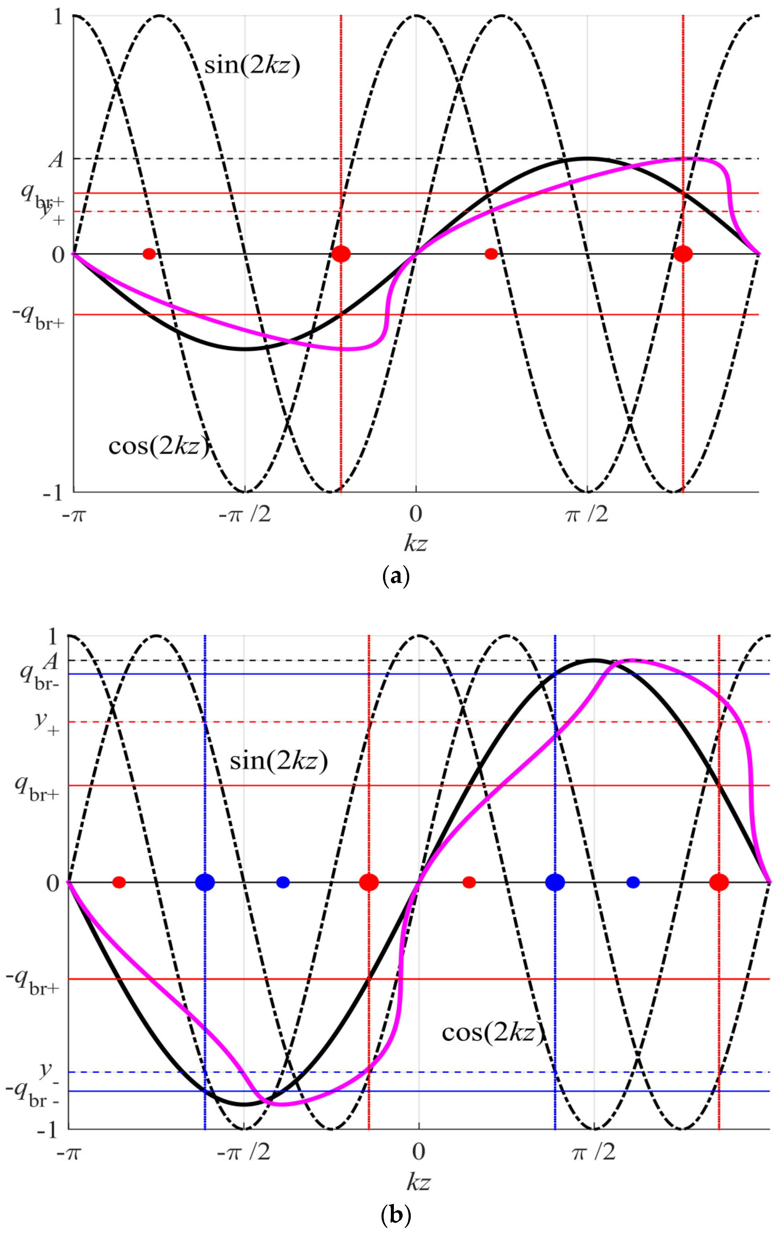
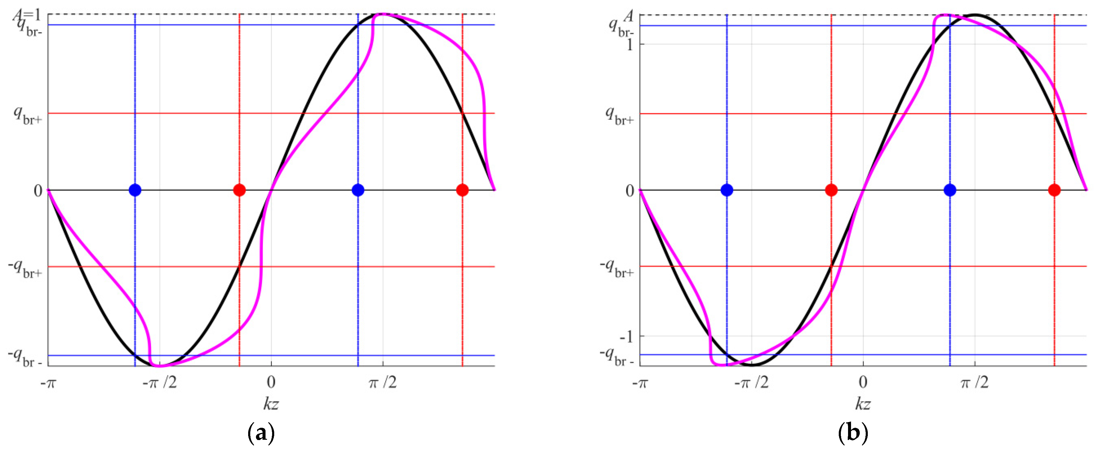
To determine the points where the shock first occurs on the Riemann wave profile, it is necessary to find the values of kz_br from relations (19) and (20) using y_± from Equation (18) for the given amplitude A. The ordinates q_br in the initial wave profile corresponding to these abscissas give us the level at which the gradient catastrophe will first occur at time moment θ = θ_br. Breaking level q_br+ is closer to the zero level, while q_br− is a larger level located closer to the crest/trough. The described algorithm for constructing points and levels of breaking is illustrated in Figure 3a for amplitude A < A*, where the only level, ±q_br+, exists, and in Figure 3b for amplitude A ∈(A*; 1), when breaking at level ±q_br− occurs later than at level ±q_br+ (θ_br− > θ_br+). Riemann waves (13) for θ = θ_br+ are also demonstrated. Wave shapes for case A = 1 (simultaneous breaking at the levels ±q_br±, θ_br− = θ_br+) and A > 1 (breaking at level ±q_br− occurs earlier than at level ±q_br+, θ_br− < θ_br+) are illustrated in Figure 4a,b.

All these features of the purely nonlinear solutions (14) are clearly observed in the numerical simulation described in Section 4 at the initial stages of wave evolution in the framework of Equation (11).

4. Numerical Simulations and Results

The study of nonlinear dynamics in the framework of Equation (11) with the initial condition (13) was carried out using numerical integration based on an implicit pseudo-spectral scheme [31] using periodic boundary conditions and including control over the numerical domain of the conservation of “mass” (I₁ = 0) and “momentum” (I₁ = A²L/2) and Hamiltonian H integrals mentioned above (Equations (3), (4), and (7), respectively). The spatial domain was chosen to equal the length of the sine wave. The numerical scheme was tested on the exact soliton solutions of the mKdV equation and stationary solutions (Equation (8)), of (2+4) KdV (in nondimesional variables, Equation (12)). In addition, the results were compared to those obtained with a doubled number of resolving points.

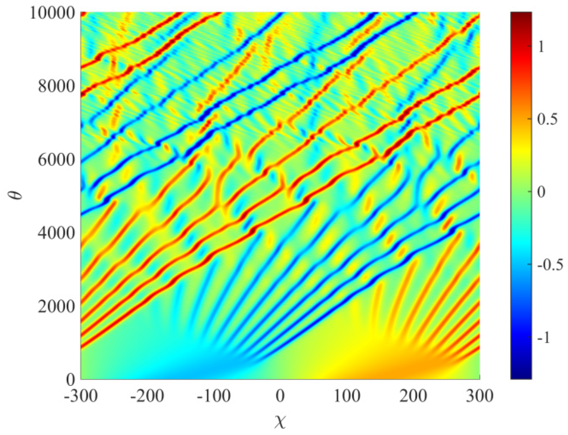
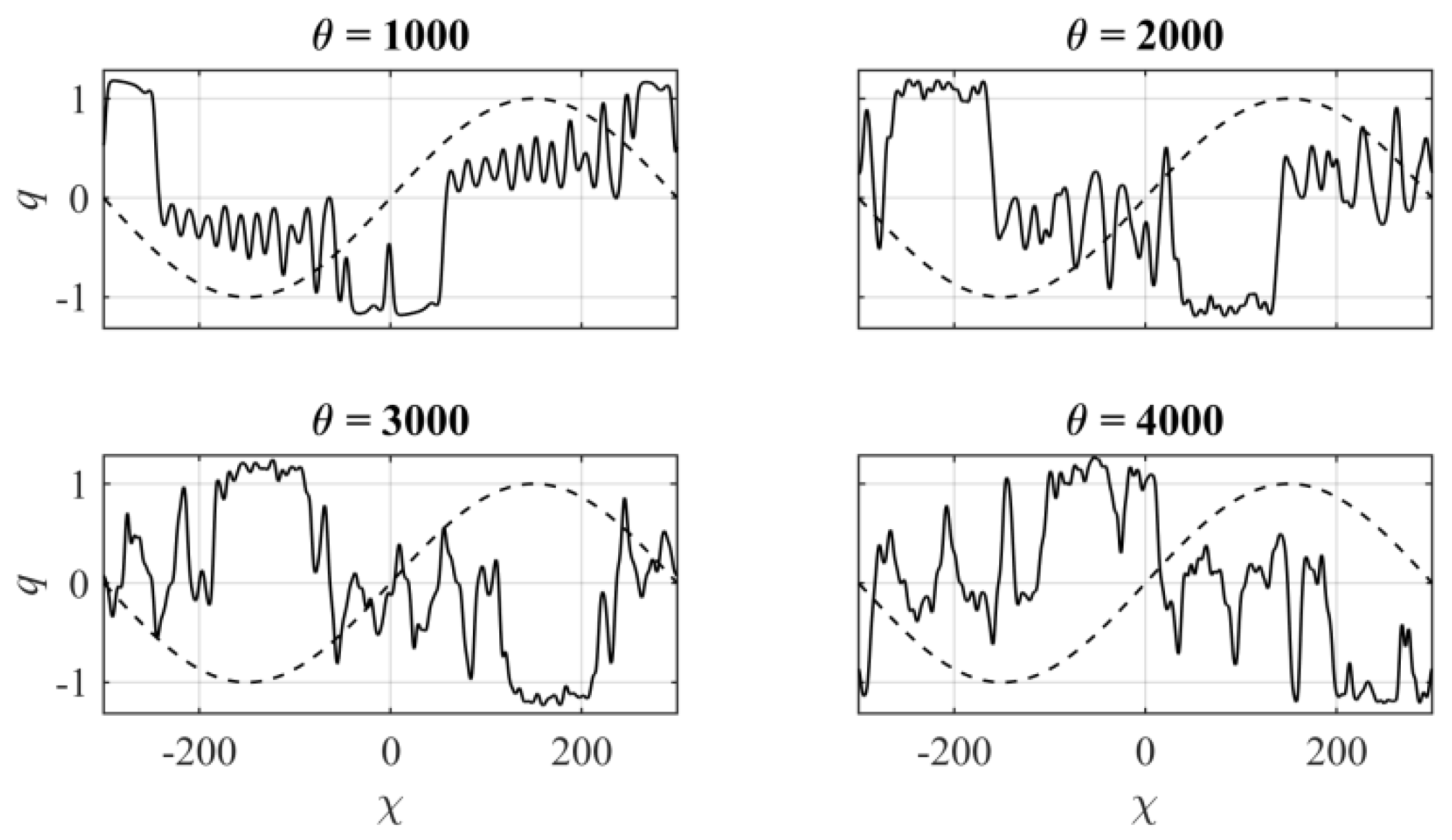
The first numerical run was performed for the initial wave of moderate amplitude (A = 0.5). From the point of view of the previous section, this case is A < A*, and steepening occurs at small times kθ < kθ_br≈ 5, most intensively on the levels of ±q_br+ ≈ 0.32 at the face slope of the wave. The initial stages of the evolving wave field at different time moments are displayed in Figure 5. The evolution scenario is similar to the scenario within the mKdV equation; the wave field is completely vertically symmetrical, but the changes within the higher-order (2+4) KdV equation occur faster. The initial harmonic wave steepens at short times due to nonlinearity; then, short-period localized perturbations of positive and negative polarities are generated. A fully undular bore was formed for θ > 2000 (kθ > 21) for this run, and due to periodicity, the collisions of solitary impulses from two neighbor periods were observed.

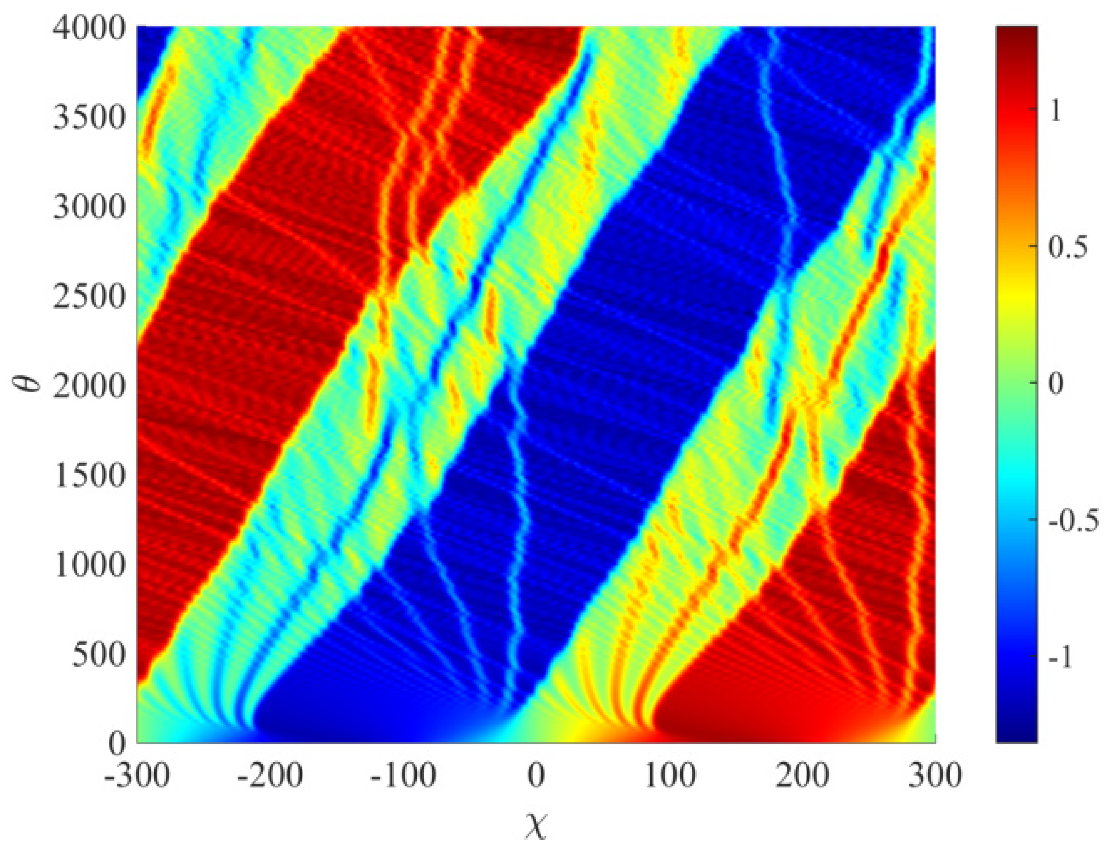
This process is also illustrated in the spacetime diagram (Figure 6), where the trajectories of the local extrema of the wave field and the phase shifts between the soliton-like waves are clearly visible. In this case, it is clearly visible that small-amplitude solitons move backward when they interact with larger-amplitude solitons. The effect of changing the direction of propagation for small solitons in the framework of the KdV-hierarchy equations was noted in [32]. Further evolution for θ ≥ 4000 in the form of snapshots is displayed in Figure 7, which illustrates how the resulting wave pattern loses symmetry and becomes irregular since many small dispersion tails appear due to nonintegrability. Inelasticity is the most pronounced in the interaction of unipolar pulses.

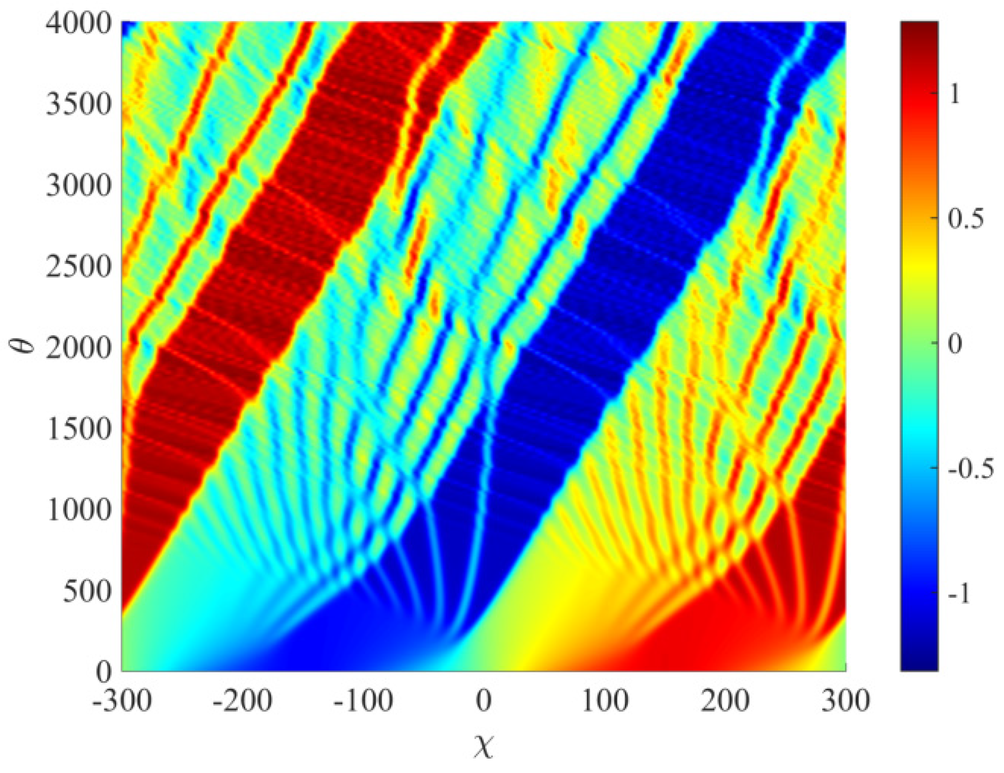
The effects of fifth-degree nonlinearity in the (2+4) KdV equation, Equation (11), become more noticeable when the amplitude of the initial wave increases. The calculation results for A = 1 are displayed in Figure 8, Figure 9 and Figure 10. A special feature of early-stage wave dynamics here (Figure 8) is the appearance of extra breaking points and, accordingly, the formation of four wave bores. This is the case when shock occurs simultaneously (at the moment θ_br± ≈ 191, kθ_br± ≈ 2) on both the back and face slopes of each half wave on the nonzero levels of ±q_br−, with q_br− ≈ 0.94, and ±q_br+, with q_br+ ≈ 0.42, respectively. Conversely, the value of the initial harmonic wave amplitude A = 1 is less than the limiting amplitude of a wide soliton q_lim ≈ 1.118, but the “thick” solitons of both polarities were generated here with amplitudes tending to (but less in absolute value than) q_lim. One can observe these “thick” solitary waves as wide red and blue stripes on the spatiotemporal plots (Figure 9). Their widths are comparable to the length, L, of the initial harmonic wave. Simultaneously, narrow solitons are generated and begin to propagate along the crests of wide solitons with a change of polarity, which is clearly visible in Figure 8, Figure 9 and Figure 10. Due to multiple collisions, the band trajectories of wide solitons deviate from linear and appear to be “trembling”.

Let us also consider the case A = 1.2 for the initial sine wave amplitude, which is larger than the limiting amplitude q_lim of the wide solitary wave. This run is illustrated by Figure 11, Figure 12 and Figure 13. Here, four breaking points are also formed (two for each of positive and negative half waves) at the levels of ±q_br−, with q_br− ≈ 1.13, and ±q_br+, with q_br+ ≈ 0.62 on the back (earlier, at θ_br− ≈ 63) and face (later, at θ_br+ ≈ 155) slopes, respectively (Figure 11). With an increase in the initial wave amplitude, the width of the “thick” solitons turns out to be larger, and for the case where A = 1.2, the total width of both positive and negative “thick” solitons exceeds half of the spatial domain (Figure 12); they occupy more than half of the length of the initial sine wave. Here, most of the interactions that small-scale solitons have with each other, and with dispersive wave “tails,” occur on the crests of the “thick” solitons as on the pedestals.

Figure 10 and Figure 13 demonstrate an increase in the number of small-scale perturbations arising and accumulating due to the inelasticity of pair and multiple interactions of solitons. Over a longer period of time, this effect can lead to the slow damping of solitary waves.

5. Conclusions

The transformation of the initial long perturbation of a sinusoidal shape in the framework of the nonintegrable version of the mKdV equation, so-called (2+4) KdV equation, which includes a combination of cubic and quintic nonlinearities, is considered. The reasonable combinations of the signs of the coefficients for nonlinear and dispersive terms were used, provided by the physical context of hydrodynamics: internal gravity waves in a fluid with symmetric vertical density stratification.

For the dispersionless version of the (2+4) KdV equation, we studied the features of the Riemann wave profile. The time for the shock to occur (breaking time), depending on the amplitude of initial sine wave, was derived in the implicit analytical form. It decreases nonlinearly with increasing wave amplitude A. The shock appears only on the face slopes for the small amplitudes (A <$\sqrt{2}/2$), while for larger amplitudes, breaking occurs at different levels on both face and back slopes. Generally, it happens at different time moments, except for A = 1, when the gradient catastrophes are simultaneous for both slopes.

Our numerical calculations within the (2+4) KdV equation demonstrate the features of the development of undular bores/solibores from the initial sine wave. As a result of its evolution, symmetric solitons of both polarities are formed, and they propagate and interact, forming a complex wave pattern. If the wave amplitude is large enough, two “thick” solitons of both negative and positive polarities are formed, in addition to bipolar groups of small-amplitude solitons passing through them. The nonlinear interactions between soliton-like pulses results in a decrease in the velocity of small-amplitude waves and, sometimes, to a change in the direction of their propagation. Multiple inelastic collisions of solitons of different polarities are accompanied by the appearance of weak irregular short waves. For longer evolutions, this effect becomes more significant and results in a distortion of trajectories and the slow damping of the solitons, breaking the symmetry of the wave field.

References

- Johnson, R.S. Water waves and Korteweg–de Vries equations. J. Fluid Mech. 1980, 97, 701–719. [Google Scholar] [CrossRef]
- Kano, T.; Nishida, T. A mathematical justification for Korteweg-de Vries equation and Boussinesq equation of water surface waves. Osaka J. Math. 1986, 23, 389–413. [Google Scholar]
- Grimshaw, R. (Ed.) Internal Solitary Waves. In Environmental Stratified Flows; Kluwer: Dordrecht, The Netherlands, 2002; pp. 1–27. [Google Scholar]
- Watanabe, S. Ion acoustic soliton in plasma with negative ion. J. Phys. Soc. Jpn. 1984, 53, 950–956. [Google Scholar] [CrossRef]
- Ruderman, M.S.; Talipova, T.; Pelinovsky, E. Dynamics of modulationally unstable ion-acoustic wave packets in plasmas with negative ions. J. Plasma Phys. 2008, 74, 639–656. [Google Scholar] [CrossRef] [Green Version]
- El-Tantawy, S.A.; Salas, A.H.; Albalawi, W. New Localized and Periodic Solutions to a Korteweg–de Vries Equation with Power Law Nonlinearity: Applications to Some Plasma Models. Symmetry 2022, 14, 197. [Google Scholar] [CrossRef]
- Demler, E.; Maltsev, A. Semiclassical solitons in strongly correlated systems of ultracold bosonic atoms in optical lattices. Ann. Phys. 2011, 326, 1775–1805. [Google Scholar] [CrossRef] [Green Version]
- Ablowitz, M.; Segur, H. Solitons and the Inverse Scattering Transform; SIAM: Philadelphia, PA, USA, 1981; 438p. [Google Scholar]
- Ablowitz, M.J.; Clarkson, P.A. Solitons, Nonlinear Evolution Equations and Inverse Scattering; Cambridge University Press: New York, NY, USA, 1991; 513p. [Google Scholar]
- Ostrovsky, L.A.; Potapov, A.I. Modulated Waves: Theory and Applications; Johns Hopkins University Press: Baltimore, MD, USA, 2002; 392p. [Google Scholar]
- Ostrovsky, L.; Pelinovsky, E.; Shrira, V.; Stepanyants, Y. Beyond the KDV: Postexplosion development. Chaos 2015, 25, 0976. [Google Scholar] [CrossRef] [PubMed]
- Kamchatnov, A.M.; Kuo, Y.H.; Lin, T.C.; Horng, T.L.; Gou, S.C.; Clift, R.; Grimshaw, R.H. Undular bore theory for the Gardner equation. Phys. Rev. E 2012, 86, 036605. [Google Scholar] [CrossRef] [PubMed] [Green Version]
- Kurkina, O.; Rouvinskaya, E.; Talipova, T.; Kurkin, A.; Pelinovsky, E. Nonlinear disintegration of sine wave: Gardner framework. Phys. D Nonlinear Phenom. 2016, 333, 222–234. [Google Scholar] [CrossRef]
- Holloway, P.; Pelinovsky, E.; Talipova, T. A generalized Korteweg–de Vries model of internal tide transformation in the coastal zone. J. Geophys. Res. 1999, 104, 18333–18350. [Google Scholar] [CrossRef] [Green Version]
- Helfrich, K.R.; Grimshaw, R.H.J. Nonlinear disintegration of the internal tide. J. Phys. Oceanogr. 2008, 38, 686–701. [Google Scholar] [CrossRef] [Green Version]
- Kurkina, O.E.; Kurkin, A.A.; Soomere, T.; Pelinovsky, E.N.; Rouvinskaya, E.A. Higher-order (2+4) Korteweg–de Vries–like equation for interfacial waves in a symmetric three-layer fluid. Phys. Fluids 2011, 23, 116602. [Google Scholar] [CrossRef]
- Kurkina, O.E.; Kurkin, A.A.; Ruvinskaya, E.A.; Pelinovsky, E.N.; Soomere, T. Dynamics of solitons in a nonintegrable version of the modified Korteweg-de Vries equation. JETP Lett. 2012, 95, 91–95. [Google Scholar] [CrossRef]
- Pelinovsky, D.E.; Grimshaw, R.H.J. An asymptotic approach to solitary wave instability and critical collapse in long-wave KdV-type evolution equations. Phys. D Nonlinear Phenom. 1996, 98, 139–155. [Google Scholar] [CrossRef]
- Zahibo, N.; Slunyaev, A.; Talipova, T.; Pelinovsky, E.; Kurkin, A.; Polukhina, O. Strongly nonlinear steepening of long interfacial waves. Nonlinear Processes Geophys. 2007, 14, 247–256. [Google Scholar] [CrossRef]
- Kartashova, E.; Pelinovsky, E.; Talipova, T. Fourier spectrum and shape evolution of an internal Riemann wave of moderate amplitude. Nonlinear Processes Geophys. 2013, 20, 571–580. [Google Scholar] [CrossRef] [Green Version]
- Pelinovsky, E.; Shurgalina, E. KDV soliton gas: Interactions and turbulence. In Advances in Dynamics, Patterns, Cognition; Aranson, I.S., Pikovsky, A., Rulkov, N.F., Tsimring, L.S., Eds.; Springer: Cham, Switzerland, 2017; pp. 295–306. [Google Scholar]
- Didenkulova, E.G. Numerical modeling of soliton turbulence within the focusing Gardner equation: Rogue wave emergence. Phys. D Nonlinear Phenom. 2019, 399, 35–41. [Google Scholar] [CrossRef]
- Marchant, T.R.; Smyth, N.F. Soliton interaction for the extended Korteweg-de Vries equation. IMA J. Appl. Math. 1996, 56, 157–176. [Google Scholar] [CrossRef]
- Martel, Y.; Merle, F. Inelastic interaction of nearly equal solitons for the quartic gKdV equation. Invent. Math. 2011, 183, 563–648. [Google Scholar] [CrossRef]
- Kodama, Y. Normal forms for weakly dispersive wave equations. Phys. Lett. A 1985, 112, 193–196. [Google Scholar] [CrossRef]
- Fokas, A.S. On a class of physically important integrable equations. Phys. D Nonlinear Phenom. 1995, 87, 145–150. [Google Scholar] [CrossRef]
- Khusnutdinova, K.R.; Stepanyants, Y.A.; Tranter, M.R. Soliton solutions to the fifth-order Korteweg–de Vries equation and their applications to surface and internal water waves. Phys. Fluids 2018, 30, 022104. [Google Scholar] [CrossRef] [Green Version]
- Hirota, R. Exact solution of the modified Korteweg-de Vries equation for multiple collisions of solitons. J. Phys. Soc. Jpn. 1972, 33, 1456–1458. [Google Scholar] [CrossRef]
- Pelinovsky, D.; Pelinovsky, E.; Kartashova, E.; Talipova, T.; Giniyatullin, A. Universal power law for the energy spectrum of breaking Riemann waves. JETP Lett. 2013, 98, 237–241. [Google Scholar] [CrossRef] [Green Version]
- Whitham, G.B. Linear and Nonlinear Waves; Wiley-Interscience Publ.: New York, NY, USA, 1974; 629p. [Google Scholar]
- Fornberg, B. A Practical Guide to Pseudospectral Methods; Cambridge University Press: Cambridge, UK, 1998; 229p. [Google Scholar]
- Shurgalina, E.G.; Pelinovsky, E.N.; Gorshkov, K.A. The effect of the negative particle velocity in a soliton gas within Korteweg–de Vries-type equations. Mosc. Univ. Phys. Bull. 2017, 72, 441–448. [Google Scholar] [CrossRef]
Figure 1.
Roots y±(A), Equation (18), providing the extrema of p(z); Equation (16) as functions of the initial wave amplitude, A.
Figure 2.
Two branches of max p(z) (a) and breaking time (b) versus initial sine wave amplitude A. The red solid curves correspond to y+ and the change of variables (19), and the blue dashed curves are computed for y− and the change of variables (20). Vertical dashed lines mark the characteristic amplitudes A = A* = , where y− starts, and A = 1, where both branches intersect.
Figure 3.
Points kzbr± (large markers, red for “+” and blue for “−”) and levels of breaking ±qbr± (solid horizontal lines, red for “+” and blue for “−”) for the Riemann wave (14) for cases A < A* (a) and A* < A < 1 (θbr− > θbr+) (b). Solid black line corresponds to initial wave , and solid magenta line corresponds to nonlinearly deformed wave . Complementary components are also illustrated; they include functions cos(2kz) and sin(2kz) (dash-dot black lines), levels of y+ (dotted lines, red for “+” and blue for “−”), and coordinates providing the minima of p(z) (small markers).
Figure 4.
Riemann waves (14) for cases A = 1 (θbr− = θbr+) (a) and A > 1 (θbr− < θbr+) (b). All notations are the same as for Figure 3, but is colored magenta in panel (b).
Figure 5.
Initial stages of the evolution of the initial disturbance, Equation (13), with A = 0.5 within the (2+4) KdV in dimensionless form (Equation (11)—black line) compared to purely nonlinear wave deformation (Equation (14)—red dashed line).
Figure 6.
Spatiotemporal evolution q(χ, θ) (values of q are illustrated in color) of the same initial wave field, Equation (13), for the case A = 0.5 in the framework of Equation (11).
Figure 7.
Snapshots of the late stage of the evolution process for A = 0.5 (the initial waveform is given by the dashed line).
Figure 8.
The same as Figure 5, but for A = 1.0.
Figure 9.
The same as Figure 6, but for A = 1.0.
Figure 10.
The same as Figure 7, but for A = 1.0.
Figure 11.
The same as Figure 5, but for A = 1.2.
Figure 12.
The same as Figure 6, but for A = 1.2.
Figure 13.
The same as Figure 7, but for A = 1.2.
Publisher’s Note: MDPI stays neutral with regard to jurisdictional claims in published maps and institutional affiliations. |
© 2022 by the authors. Licensee MDPI, Basel, Switzerland. This article is an open access article distributed under the terms and conditions of the Creative Commons Attribution (CC BY) license (https://creativecommons.org/licenses/by/4.0/).
Share and Cite
MDPI and ACS Style
Kurkina, O.; Pelinovsky, E. Nonlinear Transformation of Sine Wave within the Framework of Symmetric (2+4) KdV Equation. Symmetry 2022, 14, 668. https://0-doi-org.brum.beds.ac.uk/10.3390/sym14040668
AMA Style
Kurkina O, Pelinovsky E. Nonlinear Transformation of Sine Wave within the Framework of Symmetric (2+4) KdV Equation. Symmetry. 2022; 14(4):668. https://0-doi-org.brum.beds.ac.uk/10.3390/sym14040668
Chicago/Turabian StyleKurkina, Oxana, and Efim Pelinovsky. 2022. "Nonlinear Transformation of Sine Wave within the Framework of Symmetric (2+4) KdV Equation" Symmetry 14, no. 4: 668. https://0-doi-org.brum.beds.ac.uk/10.3390/sym14040668
Note that from the first issue of 2016, this journal uses article numbers instead of page numbers. See further details here.