Rapid Electromagnetic Modeling and Simulation of Eddy Current NDE by MLKD-ACA Algorithm with Integral Kernel Truncations

Abstract

In this article, a novel hybrid method of multilevel kernel degeneration and adaptive cross approximation (MLKD-ACA) algorithm with integral kernel truncations is proposed to accelerate solving integral equations using method of moments (MoM), and to simulate the 3D eddy current nondestructive evaluation (NDE) problems efficiently. The MLKD-ACA algorithm with an integral kernel-truncations-based fast solver is symmetrical in the sense that: (1) the impedance matrix, which is generated by the MoM representing the interactions among the field and source basis functions, is symmetrical; (2) the factorized form of the integral kernel (Green’s function) resulted from degenerating it by the Lagrange polynomial interpolation is symmetrical; (3) the structure of the truncated integral kernel for the interactions among the blocks, which ignores the trivial ones of the far block pairs, is symmetrical using the integral kernel truncations technique. The impedance variations predicted by the proposed symmetrical eddy current NDE solver are compared with other methods in benchmarks to show the remarkable accuracy and efficiency.

1. Introduction

In the field of electromagnetic nondestructive testing (EMNDT), eddy current testing (ECT) is applied widely in industry due to its sensitivity to the small discontinuities created by the defects near the surface of the conductor [1,2]. Efficient electromagnetic modeling and simulation of ECT become critical because it gives a better understanding of the involved physics and also increases the defect analysis reliability [3]. Integral equation methods are preferred for modeling and simulating the ECT problems due to their high computation precision with small number of discretized unknowns. CIVA, which is based on the volume integral equation method using the Green’s dyadic formalism, is a fast and powerful multi-technique platform [4]. The surface integral equation method is also an efficient tool to model and simulate the ECT problems with the help of method of moments (MoM) [5].

However, the main drawback of MoM is the quadratic complexity for memory requirement and cubical complexity for CPU time with direct solvers, which is a huge cost for the multiscale ECT problems [6]. Fast algorithms have been applied to alleviate the computational burden of MoM, such as the multilevel fast multipole algorithm (MLFMA) [7,8], the adaptive cross approximation algorithm (ACA) [9,10,11], fast Fourier transform method (FFT) [12], and $\mathscr{H}$ matrix algorithm [13,14,15]. MLFMA is one of the most successful fast algorithms, which is based on the addition theorem for spherical harmonics, with $O\left(N\log N\right)$ complexity [7,8]. ACA algorithm draws lots of attention due to its feature of being purely algebraic and is easy to implement into the existing codes [9,10,11]. For a low-rank matrix Z with dimension m × n, ACA algorithm generates the U and V matrices with dimensions m × r and r × n, which resulting in the computational cost to be $r^2\left(m+n\right)$, here r is the rank to approximate Z necessarily with a predefined tolerance. FFT projects the current basis functions to regular grids by interpolation to produce the same fields as the original currents [12]. $\mathscr{H}$ matrix algorithm provides an efficient mathematical framework to categorize the blocks into admissible and inadmissible ones. The inadmissible blocks are computed by full matrices and the admissible blocks are approximated by the low rank matrix compression techniques [13,14,15].

In [11], only the MLACA algorithm is applied to accelerate solving the BEM model of EMNDT; however, for the planar case, this solver lacks user friendliness [15]. In [15], a single-level kernel degeneration algorithm is proposed, while a multilevel one with a kernel truncation technique is proposed here. In this article, the novel and symmetrical hybrid method of MLKD-ACA algorithm with integral kernel truncations is proposed to model and simulate the ECT problems. The robust Stratton–Chu formulation with low frequency and high conductivity approximations are selected as the integral equations [2]. The discretized impedance matrix is symmetrical, which represents the interactions between field and source points. To apply the fast algorithm, the entire object being analyzed is enclosed in a cube and then partitioned into smaller ones recursively until the number of unknowns in each one satisfies the requirement. The block pairs are categorized into far, near and diagonal block ones symmetrically decided by the distance between blocks across the levels. Due to the nature of the integral kernel function, the far block pair interactions at each level are the low-rank matrices which can be compressed by the MLKD-ACA algorithm with kernel truncations. The interactions at leaf level are truncated, which ensures that only part of them need to be computed and stored permanently, while the ones at higher levels can be achieved with the help of the transfer matrices. Numerical experiments show both the accuracy and efficiency of the proposed fast solver.

The remainder of this article is organized as follows: in Section 2, the proposed MLKD-ACA algorithm with kernel truncations is discussed in detail. Numerical experiments are presented to demonstrate the accuracy and efficiency of the proposed fast solver to deal with the ECT problems in Section 3. The conclusion is drawn in Section 4.

2. Description of MLKD-ACA with Kernel Truncations

The Stratton–Chu formulation can be found in [16]

$$\mathbf{E}(\mathbf{r})={\mathbf{E}}^{inc}(\mathbf{r})+{\displaystyle \underset{S}{\oint }\left\{\left[\hat{\mathbf{n}}·\mathbf{E}({\mathbf{r}}^{\prime })\right]{\nabla }^{\prime }G(\mathbf{r},{\mathbf{r}}^{\prime })+\left[\hat{\mathbf{n}}\times \mathbf{E}({\mathbf{r}}^{\prime })\right]\times {\nabla }^{\prime }G(\mathbf{r},{\mathbf{r}}^{\prime })-j\omega \mu G(\mathbf{r},{\mathbf{r}}^{\prime })\left[\hat{\mathbf{n}}\times \mathbf{H}({\mathbf{r}}^{\prime })\right]\right\}}d{S}^{\prime },$$

(1)

$$\mathbf{H}(\mathbf{r})={\mathbf{H}}^{inc}(\mathbf{r})+{\displaystyle \underset{S}{\oint }\left\{j\omega \epsilon G(\mathbf{r},{\mathbf{r}}^{\prime })\left[\hat{\mathbf{n}}\times \mathbf{E}({\mathbf{r}}^{\prime })\right]+\left[\hat{\mathbf{n}}·\mathbf{H}({\mathbf{r}}^{\prime })\right]{\nabla }^{\prime }G(\mathbf{r},{\mathbf{r}}^{\prime })+\left[\hat{\mathbf{n}}\times \mathbf{H}({\mathbf{r}}^{\prime })\right]\times {\nabla }^{\prime }G(\mathbf{r},{\mathbf{r}}^{\prime })\right\}}d{S}^{\prime },$$

(2)

where ${\mathbf{E}}^{inc}$ and ${\mathbf{H}}^{inc}$ are the incident electromagnetic fields, $\mathbf{r}$ and ${\mathbf{r}}^{\prime }\in S$ are the field and source points in the domain of interest, respectively. ${\nabla }^{\prime }$ is the gradient with respect to ${\mathbf{r}}^{\prime }$. The Green function $G(\mathbf{r},{\mathbf{r}}^{\prime })=e^{-jk\left|\mathbf{r}-{\mathbf{r}}^{\prime }\right|}/\left(4\pi \left|\mathbf{r}-{\mathbf{r}}^{\prime }\right|\right)$ is the integral kernel of Stratton–Chu formulation. $k=\omega \sqrt{\mu \epsilon }$ is the wavenumber, where $\omega$, $\mu$ and $\epsilon$ are the angular frequency, permeability, and permittivity, respectively.

2.1. Multilevel Partition

The impedance matrix represents the interactions between the field and source basis functions. The whole impedance matrix is full rank, while the well-separated far block interactions are low-rank matrices, which is due to the nature of the kernel function, and they can be decomposed. Thus, the impedance matrix is represented in an approximated form which can be used for fast matrix vector multiplication in iterative solvers such as the generalized minimal residual algorithm (GMRES) or conjugate gradient (CG) [17,18].

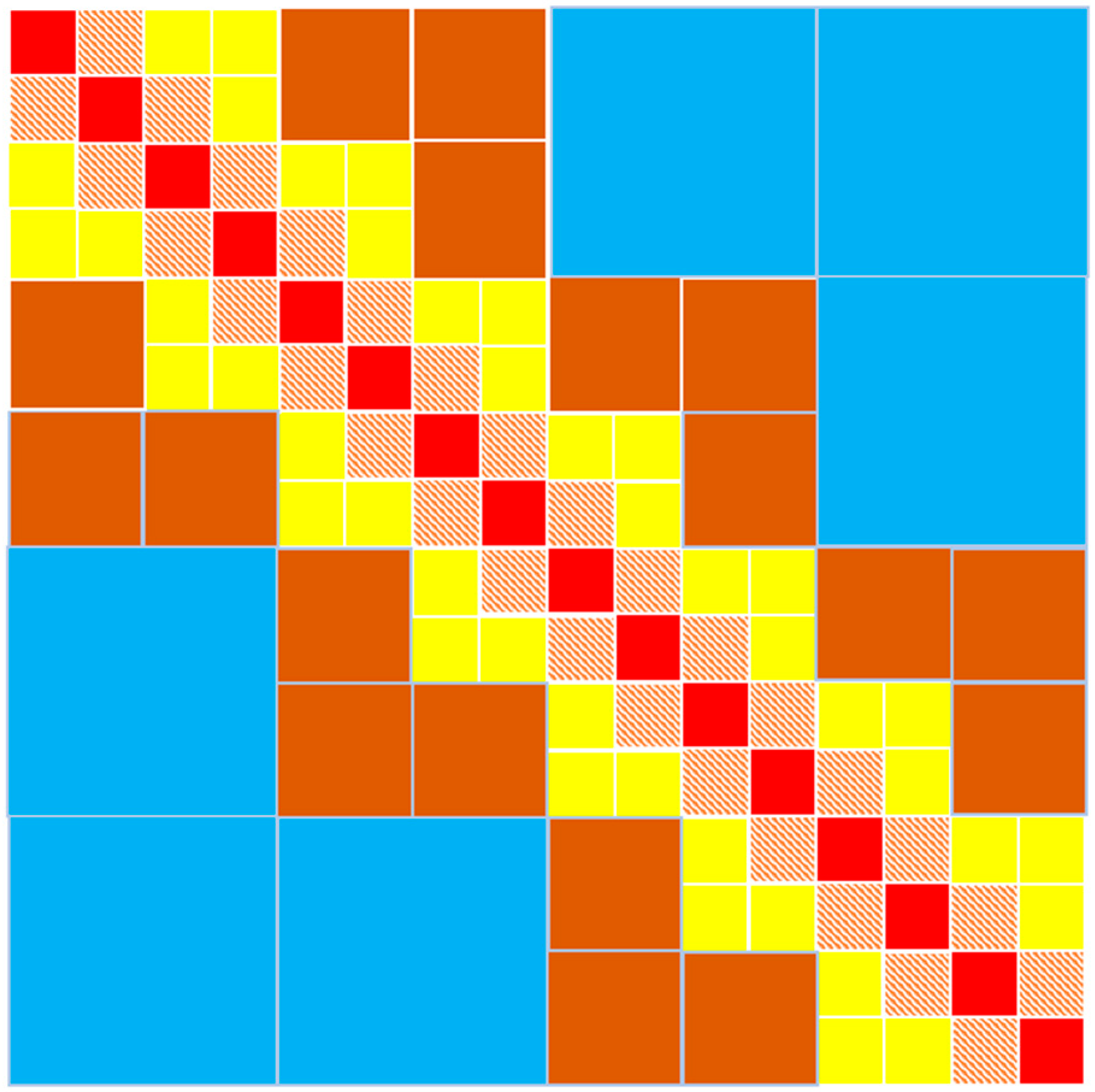
To find the well-separated blocks, the object being analyzed needs to be subdivided into blocks hierarchically. A cube is used to wrap the entire object with dimension dim, and it is subdivided recursively into $2^{l\times \dim }$ cubes at level l. At the peer level, block pairs are classified into diagonal, near, and far pairs based on the relative position of the blocks. The diagonal block pairs are the overlapped blocks, the near ones are the adjacent blocks, and the far ones are the rest of the pairs. The schematic diagram of the block pairs across the levels is shown in Figure 1. It can be found that the diagram is symmetrical with respect to the diagonal block pairs marked in red. The red shaded blocks are the near block pairs adjacent to the diagonal ones. The yellow, orange, and blue blocks are the far block pairs across the levels. The MLKD-ACA algorithm with kernel truncations can be applied to compress the far block pairs across the levels efficiently.

2.2. MLKD Algorithm

Consider the interaction of far block pair t and s, the Green function can be degenerated as [15]

$$G_{}^{t,s}\left(\mathbf{r},{\mathbf{r}}^{\prime }\right)={\displaystyle \sum _{\upsilon \in K^t}{\displaystyle \sum _{\mu \in K^s}{L}_{\upsilon }^t\left(\mathbf{r}\right)G\left({\xi }_{\upsilon }^t,{\xi }_{\mu }^s\right)}}{L}_{\mu }^s\left({\mathbf{r}}^{\prime }\right),$$

(3)

where $K:={\left\{1,2,\dots ,p\right\}}^3$ for 3D problems and p represents the interpolation points in each dimension. ${\xi }_{\upsilon }^t$ and ${\xi }_{\mu }^s$ are the families of interpolations. L is the Lagrange interpolation polynomials for field and source points, is symmetrically respect to $G\left({\xi }_{\upsilon }^t,{\xi }_{\mu }^s\right)$. The kernel degeneration algorithm owns the advantages that it separates the double integral of field and source points into two single integrals and also the Green function is represented in an accurate factorized form.

In the discretized impedance matrix, K, L and R operators shown in Equations (1) and (2) relate to the Green function [10]

$$\mathbf{K}\left(\mathbf{X}\right)=P.V.{\displaystyle \underset{S}{\oint }\nabla G\left(\mathbf{r},{\mathbf{r}}^{\prime }\right)\times \mathbf{X}\left({\mathbf{r}}^{\prime }\right)}d{S}^{\prime },$$

(4)

$$\mathbf{L}\left(\mathbf{X}\right)={\displaystyle \underset{S}{\oint }G\left(\mathbf{r},{\mathbf{r}}^{\prime }\right)\mathbf{X}\left({\mathbf{r}}^{\prime }\right)}d{S}^{\prime },$$

(5)

$$\mathbf{R}\left(X_n\right)=P.V.{\displaystyle \underset{S}{\oint }\nabla G\left(\mathbf{r},{\mathbf{r}}^{\prime }\right)X_n\left({\mathbf{r}}^{\prime }\right)}d{S}^{\prime }.$$

(6)

where P.V. stands for the principal value of the integral. The kernel functions of the K, L and R operators for the far block interactions in the submatrices ${\mathbf{R}}_1^{\times }$, $-{\mathbf{R}}_2^n$, $-{\mathbf{K}}_1^{\times }$, ${\mathbf{K}}_2^{\times }$, ${\mathbf{K}}_2^n{\mu }_2/{\mu }_1$, ${\mathbf{L}}_2^{\times }{\mu }_2/{\mu }_1$, and $-k_2^2{\mathbf{L}}_2^n$ can be degenerated accordingly [10].

The interaction of far block pair t and s in the submatrix ${\mathbf{R}}_1^{\times }$ is

$$R_{1mn}^{\times }={\displaystyle \underset{S_m}{\int }dS}\left[{\mathsf{\Lambda }}_m\left(\mathbf{r}\right)\times \hat{\mathbf{n}}\right]·{\displaystyle \underset{T_n}{\int }\nabla G_1\left(\mathbf{r},{\mathbf{r}}^{\prime }\right)b_n\left({\mathbf{r}}^{\prime }\right)d{S}^{\prime }},$$

(7)

where ${\mathsf{\Lambda }}_m\left(\mathbf{r}\right)$ is the RWG basis function [19] defined on $S_m$ for edge m, $b_n\left(\mathbf{r}\right)$ is the pulse basis function defined on $T_n$ for patch n, m is the certain edge-based basis function, and n is the certain patch-based basis functions, $\hat{\mathbf{n}}$ is the unit normal vector. $R_{1mn}^{\times }$ at the leaf level can be approximated as [15]

$${\mathbf{R}}_1^{\times }\approx {\mathbf{c}}^{a\times }·{\mathbf{g}}_1{d}_{}^{b\mathbf{T}},$$

(8)

where

$${\mathbf{c}}_{m\upsilon }^{a\times }={\displaystyle \underset{S_m}{\int }{\mathsf{\Lambda }}_m\left(\mathbf{r}\right)\times \hat{\mathbf{n}}{L}_{\upsilon }^t\left(\mathbf{r}\right)dS},$$

(9)

$${\mathbf{g}}_1=\nabla G_1\left({\xi }_{\upsilon }^t,{\xi }_{\mu }^s\right),$$

(10)

$$d_{n\mu }^b={\displaystyle \underset{T_n}{\int }{b}_n\left({\mathbf{r}}^{\prime }\right)L_{\mu }^s\left({\mathbf{r}}^{\prime }\right)dS}.$$

(11)

Because number of interpolation points is much smaller than that of the basis functions in the field and source blocks, computational costs can be decreased instead of computing the full matrix.

At coarser levels, only coupling and transfer matrices need to be calculated. The L at coarser levels can be represented by the transfer matrices

$$L_{{\upsilon }^{\prime }}^{t^{\prime }}\left(\mathbf{r}\right)={\displaystyle \sum _{\upsilon \in K^t}{E}_{{\upsilon }^{\prime }\upsilon }^t}{L}_{\upsilon }^t\left(\mathbf{r}\right),$$

(12)

$$L_{{\mu }^{\prime }}^{s^{\prime }}\left({\mathbf{r}}^{\prime }\right)={\displaystyle \sum _{\mu \in K^s}{E}_{{\mu }^{\prime }\mu }^s}{L}_{\mu }^s\left({\mathbf{r}}^{\prime }\right),$$

(13)

where $E_{{\upsilon }^{\prime }\upsilon }^t=L_{{\upsilon }^{\prime }}^{t^{\prime }}\left({\xi }_{\upsilon }^t\right)$, $E_{{\mu }^{\prime }\mu }^s=L_{{\mu }^{\prime }}^{s^{\prime }}\left({\xi }_{\mu }^s\right)$, t′ and s′ are the parents of t and s, v′ is the family of interpolation points in t′, and ${\mu }^{\prime }$ is the family of interpolation points in s′.

c and d at coarser levels can be accessed by those at leaf level and the transfer matrices

$$\begin{array}{ll}{\mathbf{c}}_{m{\upsilon }^{\prime }}^{a\times }& ={\displaystyle \underset{S_m}{\int }{\mathsf{\Lambda }}_m\left(\mathbf{r}\right)\times \hat{\mathbf{n}}{L}_{{\upsilon }^{\prime }}^{t^{\prime }}\left(\mathbf{r}\right)dS}\\ & ={\displaystyle \sum _{\upsilon \in K^t}{E}_{{\upsilon }^{\prime }\upsilon }^t{\displaystyle \underset{S_m}{\int }{\mathsf{\Lambda }}_m\left(\mathbf{r}\right)\times \hat{\mathbf{n}}{L}_{\upsilon }^t\left(\mathbf{r}\right)dS}}\\ & ={\displaystyle \sum _{\upsilon \in K^t}{E}_{{\upsilon }^{\prime }\upsilon }^t{\mathbf{c}}_{m\upsilon }^{a\times }},\end{array}$$

(14)

$$\begin{array}{ll}{d}_{n{\mu }^{\prime }}^b& ={\displaystyle \underset{S_n}{\int }{b}_n\left({\mathbf{r}}^{\prime }\right)L_{{\mu }^{\prime }}^{s^{\prime }}\left({\mathbf{r}}^{\prime }\right)d{S}^{\prime }}\\ & ={\displaystyle \sum _{\mu \in K^s}{E}_{{\mu }^{\prime }\mu }^s}{\displaystyle \underset{S_n}{\int }{b}_n\left({\mathbf{r}}^{\prime }\right)L_{\mu }^s\left({\mathbf{r}}^{\prime }\right)d{S}^{\prime }}\\ & ={\displaystyle \sum _{\mu \in K^s}{E}_{{\mu }^{\prime }\mu }^s{d}_{n\mu }^a}.\end{array}$$

(15)

The MLKD algorithm is applied to submatrices of $-k_2^2{\mathbf{L}}_2^n$, $-{\mathbf{R}}_2^n$, $-{\mathbf{K}}_1^{\times }$, and ${\mathbf{K}}_2^{\times }$. For other three submatrices, the MLACA algorithm with kernel truncations is applied.

2.3. MLACA Algorithm with Kernel Truncations

Suppose the interaction matrix Z of far block pair t and s is with dimension T by S. Application of the ACA algorithm yields the following approximate factorization [9,10,11,20,21,22,23,24,25]

$${\mathbf{Z}}_{t,s}=\mathbf{U}\times \mathbf{V}.$$

(16)

Unlike the LU decomposition, only the selected rows and columns of Z are calculated in ACA. The dimensions of U and V matrices are T by rank and rank by S, respectively. Since the rank is much smaller than T or S, only rank × (T + S) elements need to be computed and stored instead of T × S.

It should be noticed that the integral kernel functions decay exponentially in the metal. This is because k has an imaginary part in the Green’s function. Thus, the interactions among far block pairs are decreasing as the distance increases. It can be found that in the Green’s function, the interactions are inverse proportional to the distance among blocks. They would be trivial at the certain distance of two far blocks or satisfy the required accuracy and could be ignored or truncated, which yields the reduction in CPU time.

The threshold value to weigh the trivial interactions can be defined as

$${\Delta }_1=\frac{\left|{\mathbf{Z}}_{ba}\right|}{\left|{\mathbf{Z}}_{aa}\right|},$$

(17)

where ${\mathbf{Z}}_{aa}$ denotes block a’s self-interaction and ${\mathbf{Z}}_{ba}$ denotes the interaction of block a and its far interaction block b.

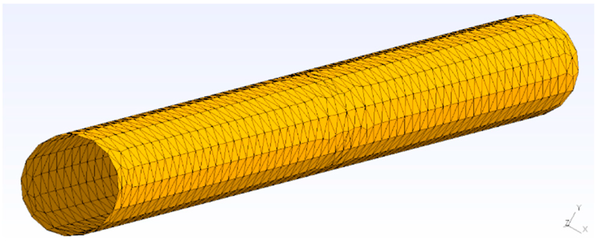
A cylinder, as shown in Figure 2, is tested numerically to show how the integral kernel truncation algorithm works. The radius of the cylinder is 1 m with the height 30 m. The object is divided into 11 non-empty blocks. With the mesh size 0.5 m, there are around 270 edge-based basis functions, and 180 patch-based basis functions in each block.

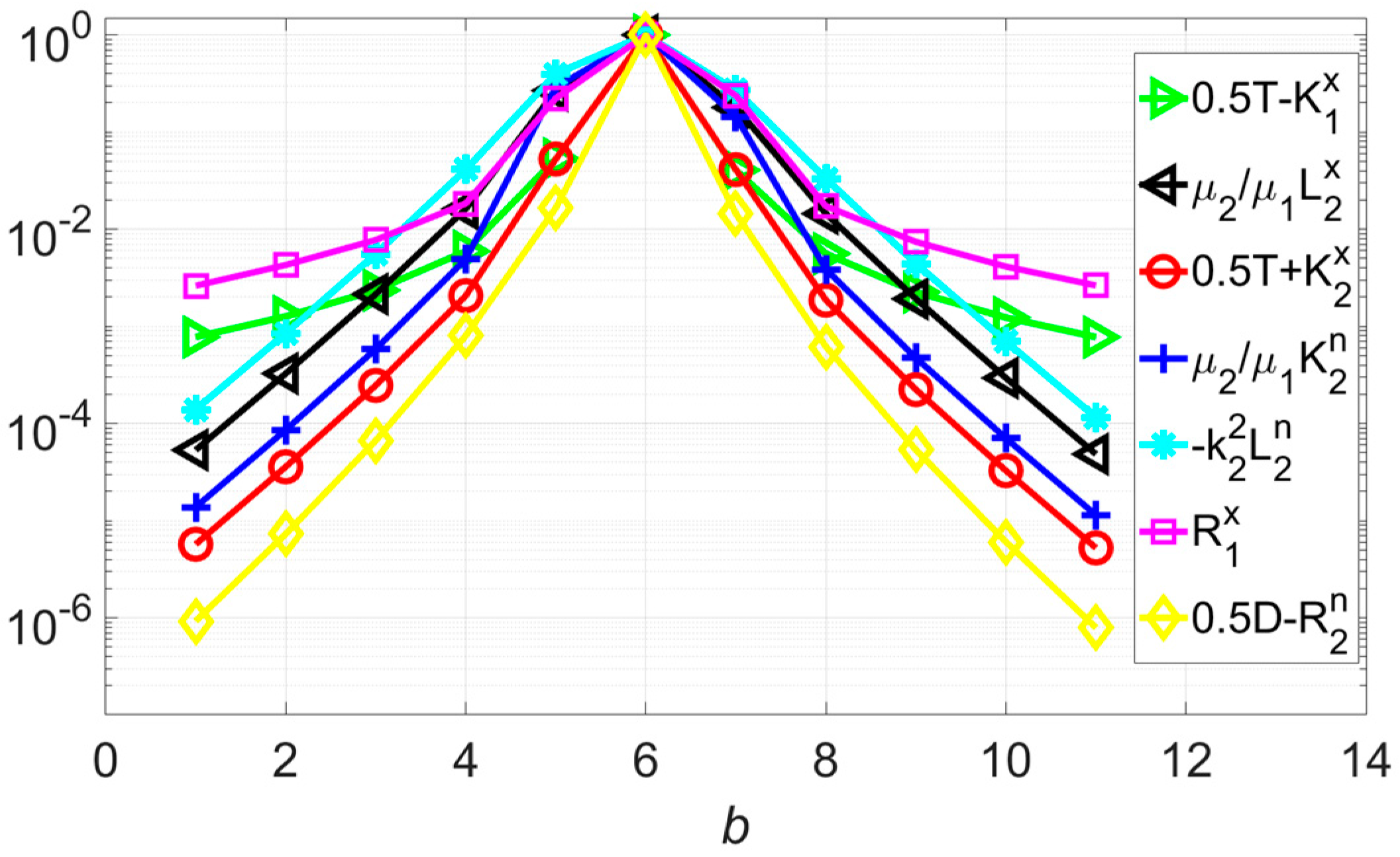
Figure 3 shows the ratios between block 6′s diagonal, near and far block interactions, and its diagonal interactions of seven submatrices. All the ratios are symmetrical with respect to b = 6 as can be seen in the figure. It can be found that for the far block pairs of block 6, as the relative distance increases, the interactions become smaller and smaller as compared with its diagonal interaction. With the required accuracy, the threshold value can be selected. At this time the trivial far block interactions can be ignored, maintaining the same solution accuracy. For example, with ${\Delta }_1={10}^{-4}$, in the submatrix related to ${\mathbf{R}}_2^n$, the interactions among block 6 and blocks 1 to 3 and 9 to 11 can be ignored. Only the interactions between block 6 and far blocks 4 and 8 need to be kept. Here, the block interactions among block 6 and block 5, 7 are near interactions and are kept. For the submatrix related to ${\mathbf{K}}_2^{\times }$, the interactions among block 6 and blocks 1, 2, 10, and 11 would be waived. Similarly, the integral kernel truncation algorithm can be applied successfully to other submatrices.

It should also be noticed that the curves associated with ${\mathbf{K}}_1^{\times }$ and ${\mathbf{R}}_1^{\times }$ operators decrease as $1/r^2$. This is because of the static behavior of the integral kernels in the air, while in the metal the curves associated with ${\mathbf{R}}_2^n$, ${\mathbf{K}}_2^{\times }$, ${\mathbf{K}}_2^n$, ${\mathbf{L}}_2^{\times }$, and ${\mathbf{L}}_2^n$ operators are decaying exponentially. To apply the kernel truncation algorithm in MLACA [11,20,21], in the first step, each interaction between the basis functions in sub-block of the source block and the field block is approximated by an ACA algorithm with kernel truncations. The maintained matrix is sent to next steps for further decomposition. The MLACA algorithm with kernel truncations accelerates the MoM solver well. This especially works for ECT problems, which usually require a large solution domain.

3. Numerical Experiments

In this section, the MLKD-ACA algorithm with integral kernel truncations is applied and implemented to solve the ECT benchmark problems. The Auld’s formulation is used to calculate the impedance variations [26]. The GMRES iterative method is used to solve the system of equations. All computations are performed in double precision on an AMD Workstation with a clock speed of 3.7 GHz. The number of levels in the multilevel algorithm is determined to maintain the certain box size at the leaf level.

3.1. Coil with Finite Cross Section Placing above a Conductive Plate

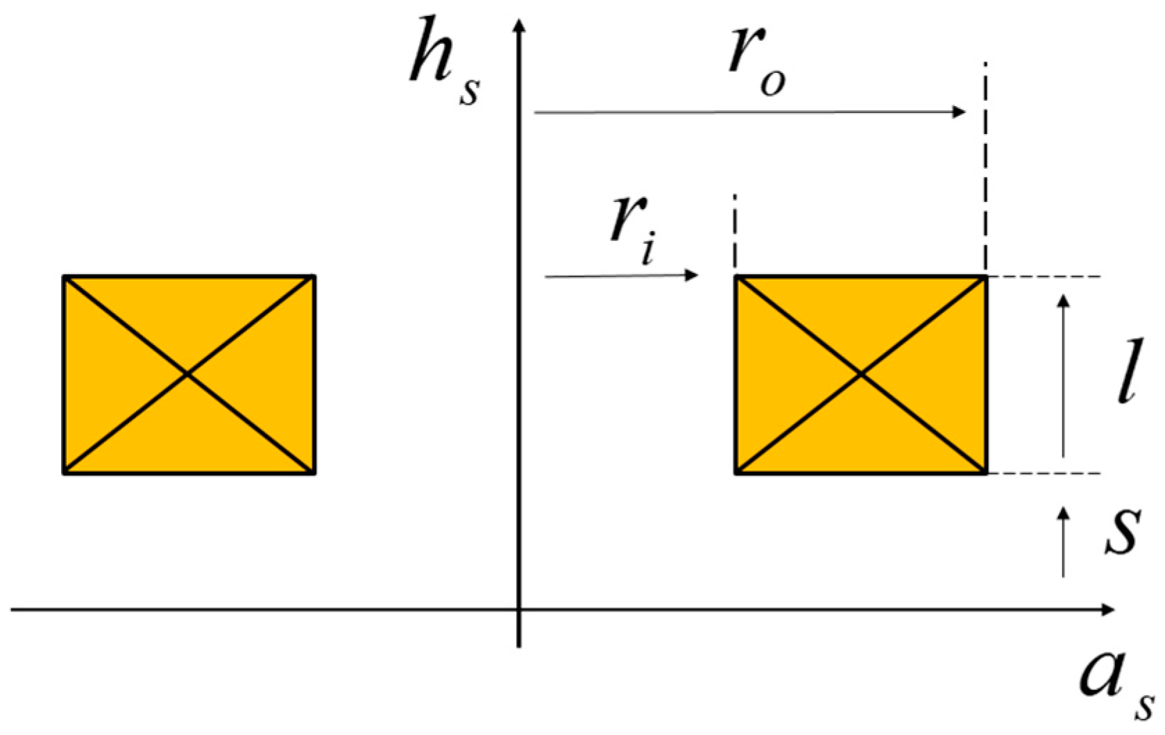
As a canonical case, the planar ECT problem is discussed first. Placing coil C5 with inner radius 9.33 mm, outer radius 18.04 mm, 1910 turns, above a healthy (no surface slot) conductive plate with conductivity 25.5 MS/m, thickness 10.05 mm and lift off 3.32 mm [27]. The coil with finite cross section is shown in Figure 4.

Four level MLKD-ACA algorithm is applied with ACA tolerance ${10}^{-2}$ and p = 1 in each block at level 2, 3, and 4. The impedance variations predicted by the MLKD-ACA algorithm with integral kernel truncations of different threshold values are compared with other solvers or methods as shown in

Table 1. Impedance variations achieved by different solvers for placing coil C5, operating at 850 Hz, above a conductive plate.

Solver or Method	$\mathbf{Impedance}\mathbf{Variation}\left(\mathsf{\Omega }\right)$
$\mathrm{MLKD}\text{-}\mathrm{ACA}\mathrm{with}{\Delta }_1={10}^{-2}$	$22.054-69.312j$
$\mathrm{MLKD}\text{-}\mathrm{ACA}\mathrm{with}{\Delta }_1={10}^{-3}$	$22.237-70.437j$
$\mathrm{MLKD}\text{-}\mathrm{ACA}\mathrm{with}{\Delta }_1={10}^{-4}$	$22.141-70.431j$
$\mathrm{MLKD}\text{-}\mathrm{ACA}\mathrm{with}{\Delta }_1={10}^{-5}$	$22.143-70.428j$
MoM [10]	$22.153-70.409j$
Experiment [27]	$20.00-70.5j$
Theodoulidis and Bowler [27]	$22.25-70.45j$
Dodd and Deeds [28]	$22.20-70.49j$

operating at 850 Hz. The agreements among the MLKD-ACA algorithm with kernel truncations solver, the MoM solver, analytical, semi-analytical methods, and experiment are good.

It can be found in Table 1 that as the threshold value decreases (${\Delta }_1={10}^{-2},{10}^{-3},{10}^{-4},{10}^{-5}$), the accuracy increases (relative differences to MoM solver are decreasing as: 1.5%, 1.2%, 0.0034%, 0.0029%); however, the efficiency is worsened: the memory requirements of the far blocks, which are truncated and tuned by ${\Delta }_1$, are increasing as can be seen in Figure 5. The savings of the far block pairs relative to MLKD-ACA algorithm without truncations are decreasing as: 79.4%, 56.1%, 38.1% and 30.5%. The threshold value can be selected for satisfying the required accuracy to ensure the best performance. In this case, MLKD-ACA with ${\Delta }_1={10}^{-4}$ is selected with the relative difference of impedance variations smaller than 1% compared with the MoM solver. In MoM, the total memory requirement is 3.36 GB and the CPU time per iteration is 0.43 s. For the performance, the proposed solver just needs 4.45% in memory and 9.2% CPU time of MoM which shows both the accuracy and efficiency.

For the case of placing coil C27 with inner radius 7.04 mm, outer radius 12.4 mm, 556 turns, above a conductive plate with conductivity 21.8 MS/m, thickness 5.04 mm, and lift off 3.43 mm. Four level MLKD-ACA algorithm is applied with ACA tolerance ${10}^{-2}$ and p = 1 in each block at level 2, 3, and 4. The impedance variations predicted by the MLKD-ACA algorithm with integral kernel truncations of different threshold values are compared with other solvers or methods as shown in

Table 2. Impedance variations achieved by different solvers for placing coil C27, operating at 20 kHz, above a conductive plate.

Solver or Method	$\mathbf{Impedance}\mathbf{Variation}\left(\mathsf{\Omega }\right)$
$\mathrm{MLKD}\text{-}\mathrm{ACA}\mathrm{with}{\Delta }_1={10}^{-1}$	$10.583-127.438j$
$\mathrm{MLKD}\text{-}\mathrm{ACA}\mathrm{with}{\Delta }_1={10}^{-2}$	$12.825-124.837j$
$\mathrm{MLKD}\text{-}\mathrm{ACA}\mathrm{with}{\Delta }_1={10}^{-3}$	$12.721-124.992j$
$\mathrm{MLKD}\text{-}\mathrm{ACA}\mathrm{with}{\Delta }_1={10}^{-4}$	$12.721-124.990j$
$\mathrm{MLKD}\text{-}\mathrm{ACA}\mathrm{with}{\Delta }_1={10}^{-5}$	$12.722-124.989j$
MoM [10]	$12.734-124.98j$
Experiment [27]	$12.650-125.1j$
Theodoulidis and Bowler [27]	$12.801-125.329j$
Dodd and Deeds [28]	$12.801-125.388j$

operating at 20 kHz. Again, good agreements among the MLKD-ACA algorithm with kernel truncations solver, the MoM solver, analytical, semi-analytical methods and experiment can be observed.

Table 2 shows that as the threshold value decreases (${\Delta }_1={10}^{-1},{10}^{-2},{10}^{-3},{10}^{-4},{10}^{-5}$), the accuracy increases (relative differences as compared with MoM solver are increasing as: 2.6%, 0.13%, 0.014%, 0.013%, 0.012%) with the worsening efficiency, as shown in Figure 6: the savings of the far block pairs relative to MLKD-ACA algorithm without truncations are decreasing as: 76.0%, 64.5%, 61.0%, and 49.9%. In this case, to ensure the best performance for the desired accuracy, the MLKD-ACA with ${\Delta }_1={10}^{-2}$ is chosen with at least two digits in agreement of the impedance variation with the one predicted by the MoM solver. In MoM, the total memory requirement is 3.43 GB and the CPU time per iteration is 0.45 s. MLKD-ACA with ${\Delta }_1={10}^{-2}$ just needs 3.2% in memory and 8.8% CPU time of MoM, which again shows the robustness and efficiency of the proposed solver.

3.2. Single Turn Coil Placing above a Conductive Sphere

After testing the planar-shaped ECT problem, the spherical one is considered. The coil operating at 500 Hz with radius 0.1 m is placed above a conducting sphere with a radius of 0.2 m and conductivity of 2.53 MS/m, as shown in Figure 7. 3 level MLKD-ACA algorithm is applied with ACA tolerance ${10}^{-2}$ and p = 1 in each block at level 2 and 3. The impedance variations predicted and memory of far block pairs required by the MLKD-ACA algorithm with integral kernel truncations of different threshold values are compared with other solvers or methods as shown in

Table 3. Impedance variations predicted, and memory of far block pairs required, by different solvers for placing single turn coil, operating at 500 Hz, above a conductive sphere.

Solver or Method	$\mathbf{Impedance}\mathbf{Variation}\left(\mathsf{\mu }\mathsf{\Omega }\right)$	Memory Requirement for Far Block Pairs (MB)
$\mathrm{MLKD}\text{-}\mathrm{ACA}\mathrm{with}{\Delta }_1={10}^{-2}$	$0.2293-1.497j$	24.8
$\mathrm{MLKD}\text{-}\mathrm{ACA}\mathrm{with}{\Delta }_1={10}^{-3}$	$0.2431-1.478j$	104.3
$\mathrm{MLKD}\text{-}\mathrm{ACA}\mathrm{with}{\Delta }_1={10}^{-4}$	$0.2422-1.478j$	151.3
$\mathrm{MLKD}\text{-}\mathrm{ACA}\mathrm{with}{\Delta }_1={10}^{-5}$	$0.2421-1.480j$	190.3
MoM [30,31]	$0.2416-1.484j$	NA
Analytical method [29]	$0.2425-1.489j$	NA

.

The good agreements among the MLKD-ACA algorithm with kernel truncations solver, the MoM solver, and the analytical method are observed in Table 3. The relative differences of the impedance variations among the MLKD-ACA algorithm with different thresholds (${\Delta }_1={10}^{-2},{10}^{-3},{10}^{-4},{10}^{-5}$) and the MoM are 1.19%, 0.41%, 0.4%, 0.27%, respectively. As the threshold increases, the memory requirements of the far block pairs decrease to 53.4%, 63.1%, 74.6%, and 93.4% compared with that of the MLKD-ACA algorithm without truncations. In MoM, it requires 17.3 GB in memory and 1.78 s in CPU time per iteration. To ensure the two-digit accuracy, the MLKD-ACA algorithm with ${\Delta }_1={10}^{-3}$ solver is selected; it only requires 4.6% and 10.1% of memory and CPU time in MoM, respectively.

3.3. Coil with Finite Cross Section Placing above a Conductive Plate with Surface Slot

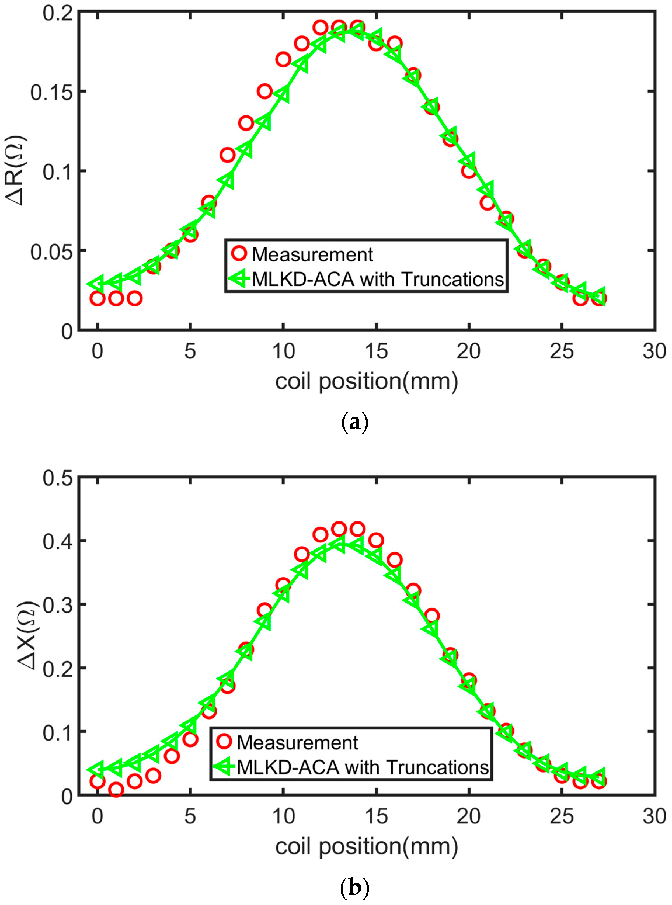
Consider the multiscale ECT problem, TEAM WORKSHOP 15 [32], as shown in Figure 8. The coil, operating at 7 kHz with 408 turns, an inner radius of 9.34 mm, an outer radius of 18.4 mm, placing above a conductive plate, with thickness of 9 mm and liftoff distance of 2.03 mm, with a surface slot of 12.6 mm in length, 5 mm in depth, and 0.28 mm in width.

In the MoM solver, the memory requirement is 614 GB which cannot be handled by our server. Thus, it goes to the MLKD-ACA algorithm with kernel truncations solver. The impedance variations, both in real and imaginary parts, when scanning the coil across the surface slot, predicted by the MLKD-ACA algorithm with kernel truncations are compared with the measurements [32] as shown in Figure 9. Excellent agreements can be found with ${\Delta }_1={10}^{-4}$ to ensure the best efficiency.

4. Conclusions

In this paper, a MLKD-ACA algorithm with an integral kernel truncations solver was proposed for simulating and modeling ECT problems. The symmetrical schematic diagram of the impedance matrix was categorized into diagonal, near, and far block pairs. The far block interactions were approximated by degenerating the integral kernel function by the Lagrange polynomials into the symmetrical factorized form. Additionally, those interactions were truncated symmetrically by applying a threshold, which costs less CPU time and has trivial influences on accuracy. The proposed solver was tested in several benchmarks and showed both remarkable robustness and efficiency. By tuning the threshold and truncating the integral kernels, the proposed solver improves the overall efficiency of the MLKD-ACA algorithm solver.

In future work, the overall performance could be further optimized through parallelization. Other kernel degeneration methods with merits should be analyzed and applied to optimize the performance of the model. With the proposed fast and efficient forward solver for ECT problems, inverse problems which aim at determining the shape and size of the flaw can be studied. Statistical learning can also be applied to construct the efficient model to relieve the computational burden of the forward solver.

References

- Lu, M.; Meng, X.; Huang, R.; Chen, L.; Tang, Z.; Li, J.; Peyton, A.; Yin, W. Determination of surface crack orientation based on thin-skin regime using triple-coil drive–pickup eddy-current sensor. IEEE Trans. Instrum. Meas. 2020, 70, 1–9. [Google Scholar] [CrossRef]
- Bao, Y.; Song, J.M. Analysis of electromagnetic non-destructive evaluation modelling using Stratton-Chu formulation-based fast algorithm. Philos. Trans. R. Soc. A 2020, 378, 20190583. [Google Scholar] [CrossRef] [PubMed]
- Pichenot, G.; Buvat, F.; Hristoforou, E. Eddy current modelling for nondestructive testing. J. Nondestruct. Test. 2003, 8, 1–5. [Google Scholar]
- Gilles-Pascaud, C.; Pichenot, G.; Premel, D.; Reboud, C.; Skarlatos, A. Modelling of eddy current inspections with CIVA. In Proceedings of the 17th World Conference on Nondestructive Testing, Shanghai, China, 25 October 2008. [Google Scholar]
- Yang, M. Efficient Method for Solving Boundary Integral Equation in Diffusive Scalar Problem and Eddy Current Nondestructive Evaluation. Ph.D. Dissertation, Iowa State University, Ames, IA, USA, 2010. [Google Scholar]
- Chew, W.C.; Tong, M.S.; Hu, B. Integral Equation Methods for Electromagnetic and Elastic Waves, 1st ed.; Morgan & Claypool: London, UK, 2008; pp. 107–160. [Google Scholar]
- Rubinacci, G.; Tamburrino, A.; Ventre, S.; Villone, F. A fast 3-D multipole method for eddy-current computation. IEEE Trans. Mag. 2004, 40, 1290–1293. [Google Scholar] [CrossRef]
- Song, J.M.; Lu, C.-C.; Chew, W.C. Multilevel fast multipole algorithm for electromagnetic scattering by large complex objects. IEEE Trans. Antennas Propag. 1997, 45, 1488–1493. [Google Scholar] [CrossRef] [Green Version]
- Bebendorf, M. Approximation of boundary element matrices. Numer. Math. 2000, 86, 565–589. [Google Scholar] [CrossRef]
- Bao, Y.; Liu, Z.W.; Song, J. Adaptive cross approximation algorithm for accelerating BEM in eddy current nondestructive evaluation. J. Nondestruct. Eval. 2018, 37, 68. [Google Scholar] [CrossRef]
- Bao, Y.; Liu, Z.W.; Bowler, J.R.; Song, J. Multilevel adaptive cross approximation for efficient modeling of 3D arbitrary shaped eddy current NDE problems. NDTE Int. 2019, 104, 1–9. [Google Scholar] [CrossRef]
- Tamburrino, A.; Ventre, S.; Rubinacci, G. A FFT integral formulation using edge-elements for eddy current testing. Int. J. Appl. Electromag. Mech. 2000, 11, 141–162. [Google Scholar] [CrossRef]
- Hackbusch, W. A sparse matrix arithmetic based on H-matrices. Part I: Introduction to H-matrices. Computing 1999, 62, 89–108. [Google Scholar] [CrossRef]
- Chai, W.W.; Jiao, D. An H2-matrix-based integral-equation solver of reduced complexity and controlled accuracy for solving electrodynamic problems. IEEE Trans. Antennas Propag. 2009, 57, 3147–3159. [Google Scholar] [CrossRef]
- Bao, Y.; Wan, T.; Liu, Z.; Bowler, J.R.; Song, J. Integral equation fast solver with truncated and degenerated kernel for computing flaw signals in eddy current non-destructive testing. NDT E Int. 2021, 124, 102544. [Google Scholar] [CrossRef]
- Stratton, J.A. Electromagnetic Theory; McGraw-Hill: New York, NY, USA, 1941. [Google Scholar]
- Saad, Y.; Schultz, M.H. GMRES: A generalized minimal residual algorithm for solving nonsymmetric linear systems. SIAM J. Sci. Stat. Comp. 1986, 7, 856–869. [Google Scholar] [CrossRef] [Green Version]
- Smith, C.F.; Peterson, A.F.; Mittra, R. A conjugate gradient algorithm for the treatment of multiple incident electromagnetic fields. IEEE Trans. Antennas Propag. 1989, 37, 1490–1493. [Google Scholar] [CrossRef]
- Rao, S.M.; Wilton, D.R.; Glisson, A. Electromagnetic scattering by surfaces of arbitrary shape. IEEE Trans. Antennas Propag. 1982, 30, 409–428. [Google Scholar] [CrossRef] [Green Version]
- Tamayo, J.M.; Heldring, A.; Rius, J.M. Multilevel adaptive cross approximation (MLACA). IEEE Trans. Antennas Propag. 2011, 59, 4600–4608. [Google Scholar] [CrossRef] [Green Version]
- Chen, X.L.; Gu, C.Q.; Ding, J.; Li, Z.; Niu, Z. Multilevel fast adaptive cross approximation algorithm with characteristic basis functions. IEEE Trans. Antennas Propag. 2015, 63, 3994–4002. [Google Scholar] [CrossRef]
- Gibson, W.C. Efficient solution of electromagnetic scattering problems using multilevel adaptive cross approximation and LU factorization. IEEE Trans. Antennas Propag. 2020, 68, 3815–3823. [Google Scholar] [CrossRef]
- Nel, B.A.P.; Botha, M.M. An efficient MLACA-SVD solver for superconducting integrated circuit analysis. IEEE Trans. Appl. Supercond. 2019, 29, 1303301. [Google Scholar] [CrossRef]
- Heldring, A.; Ubeda, E.; Rius, J.M. Improving the accuracy of the adaptive cross approximation with a convergence criterion based on random sampling. IEEE Trans. Antennas Propag. 2021, 69, 347–355. [Google Scholar] [CrossRef]
- Liu, Y.; Sid-Lakhdar, W.; Rebrova, E.; Ghysels, P.; Li, X.S. A parallel hierarchical blocked adaptive cross approximation algorithm. Int. J. High Perform. Comput. Appl. 2022, 34, 394–408. [Google Scholar] [CrossRef]
- Auld, B.A.; Moulder, J.C. Review of advances in quantitative eddy current nondestructive evaluation. J. Nondestruct. Eval. 1999, 18, 3–36. [Google Scholar] [CrossRef]
- Theodoulidis, T.P.; Bowler, J.R. Eddy current coil interaction with a right-angled conductive wedge. Proc. R. Soc. 2005, 461, 3123–3139. [Google Scholar] [CrossRef]
- Dodd, C.V.; Deeds, W.E. Analytical solutions to eddy-current probe-coil problems. J. Appl. Phys. 1968, 39, 2829–2838. [Google Scholar] [CrossRef] [Green Version]
- Antimirov, M.Y.; Kolyshkin, A.A.; Vaillancourt, R. Mathematical Models for Eddy Current Testing; Les Publications CRM: Montreal, QC, Canada, 1997; pp. 107–114. [Google Scholar]
- Bao, Y.; Song, J.M. Multilevel kernel degeneration–adaptive cross approximation method to model eddy current NDE problems. J. Nondestruct. Eval. 2022, 41, 17. [Google Scholar] [CrossRef]
- Bao, Y.; Liu, Z.W.; Bowler, J.R.; Song, J. Nested kernel degeneration-based boundary element method solver for rapid computation of eddy current signals. NDTE Int. 2022, 128, 102633. [Google Scholar] [CrossRef]
- Sabbagh, H.A.; Burke, S.K. Benchmark problems in eddy-current NDE. In Proceedings of the Review of Progress in Quantitative Nondestructive Evaluation, Brunswick, ME, USA, 2 August 1992. [Google Scholar]
Figure 1.
Symmetrical schematic diagram of the block pairs across the levels.
Figure 2.
A cylinder with flat triangle meshes.
Figure 3.
The ratios between block 6′s diagonal, near and far interactions, and its diagonal interactions of seven submatrices.
Figure 4.
A coil with finite cross section. and represent the inner and outer radii of the coil, respectively. S is the lift-off distance between the coil and the conducting plate. l is the thickness of the coil. and are the continuous variables in the radial and vertical directions, respectively [2].
Figure 5.
Case of placing coil C5 above the conductive plate. Memory requirements for total and far block interactions of MLKD-ACA algorithm with threshold values of kernel truncations.
Figure 6.
Case of placing coil C27 above the conductive plate. Memory requirements for total and far block interactions of MLKD-ACA algorithm with threshold values of kernel truncations.
Figure 7.
Problem description of placing single turn coil above a conducting sphere [29]. R0 and R1 represent the free space and conducting sphere. The radius of the single turn coil is with lift-off distance h between the coil and the sphere with radius . is the distance between the origin of the sphere and the edge of the coil.
Figure 8.
A coil with finite cross section placing above a conducting plate with a surface slot.
Figure 9.
Impedance variations of scanning the coil above the conductive plate with surface slot predicted and measured by the MLKD-ACA algorithm with kernel truncations solver and measurements: (a) Resistance variations; (b) reactance variations.