All articles published by MDPI are made immediately available worldwide under an open access license. No special
permission is required to reuse all or part of the article published by MDPI, including figures and tables. For
articles published under an open access Creative Common CC BY license, any part of the article may be reused without
permission provided that the original article is clearly cited. For more information, please refer to
https://0-www-mdpi-com.brum.beds.ac.uk/openaccess.
Feature papers represent the most advanced research with significant potential for high impact in the field. A Feature
Paper should be a substantial original Article that involves several techniques or approaches, provides an outlook for
future research directions and describes possible research applications.
Feature papers are submitted upon individual invitation or recommendation by the scientific editors and must receive
positive feedback from the reviewers.
Editor’s Choice articles are based on recommendations by the scientific editors of MDPI journals from around the world.
Editors select a small number of articles recently published in the journal that they believe will be particularly
interesting to readers, or important in the respective research area. The aim is to provide a snapshot of some of the
most exciting work published in the various research areas of the journal.
Evaluation of Coastal Zone Construction Based on Theories of the Combination of Empowerment Judgment and Neural Networks: The Example of the Putian Coastal Zone
Coastal engineering construction suitability evaluation methods are too empirical and difficult to quantify. Considering these weaknesses, in order to determine the weight of each factor reasonably, and to analyze the suitability of coastal zone construction comprehensively, the theory of establishing a coastal zone construction suitability evaluation model based on a Rough Set (RS) and an Analytic Hierarchy Process (AHP) is proposed. In total, 20 typical coastal areas of Putian are selected, and the main impact factors are determined according to a port dock, pollution-prone industry, and an electric power plant. The contribution rate and weight of each factor for the construction of a coastal zone are analyzed by the combination evaluation model, and the final evaluation result is consistent with the actual investigation situation. Finally, 52 evaluation units of the Putian coastal zone are evaluated by Neural Networks (NNs). The weight of the impact factors is made more objective by using the training sample set of the combination evaluation model as the sample set of the neural network. The learning speed and accuracy of the network are improved, and the and the evaluation result is consistent with the actual investigation situation. In a word, it is effective to perform the suitability evaluation of the coastal zone construction using the RS-AHP-NN proposed model, and it can be applied in practical engineering.
The coastal zone is a transition zone between the ocean and a specific collection of land and marine spaces; it is a mutual transition zone between the lithosphere, hydrosphere, atmosphere and biosphere, with the most frequent exchanges. It has a wealth of resources and services that are vital to human social and economic development [1]. In the world, coastal cities tend to be the most developed areas in the country. But at the same time, the coastal zone has disasters and fragile ecological characteristics. Given this, how can we realize a scientific and objective coastal construction suitability evaluation, which is the basic problem of the port area and the surrounding coastal zone in the planning and construction layout [2]? Especially at present, China’s “The Belt and Road Initiative” plan has been proposed to become a major strategic initiative of national revival development and one of the major opportunities of global development; coastal zone development and engineering construction are important parts of the planning. As such, the science of the coastal zone construction suitability evaluation method and system research are more urgent and important.
In recent years, a variety of methods and models have been applied to the evaluation of engineering construction. For example, Tie et al. used AHP to give weight to different assessment indicators, and established the assessment model of disaster emergency response capabilities in urban settings [3].Yang analyzed the probability distribution rule of the strain ratio using the random signal analysis theory and statistical technology, and Gong summarized the impact on environment quality in the process of relocation according to the statistical analysis of the environmental monitoring data [4,5]. As the conventional prediction methods for the production of water flooding reservoirs have some drawbacks, a production forecasting model based on an artificial neural network was proposed [6]. Chen proposed a construction quality evaluation model based on the genetic algorithm, and Qi combined the genetic algorithm and analytic hierarchy process in view of the lack of objectiveness and the low credibility of the results of current construction quality evaluation [7,8]. Chen by applying hierarchical analysis and fuzzy mathematical theory, thus providing a comprehensive evaluation of the mine environment [9]; Liang et al. fully considered the fuzziness and uncertainty of data, and the fusion evaluation of cracks was proposed based on an improved cloud-evidence theory [10]. Wu analyzed the main factors affecting the expansion of urban land in Zhumadian City, and established an evaluation index system for the urban expansion of the city; Xie used an extended multi-factor assessment method to construct an assessment model that accurately reflects the service quality of urban public transportation [11,12]. However, on the one hand, coastal engineering construction is a subject of engineering geological conditions, terrain conditions and some unstable factors to control the extremely complex geological processes, such as special rock and soil. This paper carried out geological survey work involving active faults, groundwater, and 12 other kinds of factors, including a lot of uncertainty and hidden factors. The methods mentioned above do not consider the factors affecting the construction of the coastal zone in a comprehensive way, and can only be semi-quantitative, or only consider the qualitative and quantitative, and cannot handle the relationship between them very well. On the other hand, in the study of natural science and engineering construction, there is a lot of uncertain information, and the evaluation of coastal engineering construction involves many variables (quantitative, semi-quantitative, and qualitative) and a large amount of data. These variables and the evaluation’s conclusion often have a highly nonlinear relationship. At present, there are some weaknesses in the approach mentioned above.
In view of this situation, this paper concerns more than 1 year of the study area of 364 square kilometers with regard to complex and uncertain factors, and determined the geological survey. The paper puts forward the analytic hierarchy process and rough set combined weight judgment matrix theory with a comprehensive evaluation method for the neural network. By this method, a model was developed for the integrated evaluation of a great deal of complex and uncertain information, and the problem of weighting the impact factors is solved. Then, the NN method is used to give full play to its great advantages of massively parallel processing, self-learning, and real-time processing to provide a new method for the engineering construction of complex coastal suitability evaluation.
In the coastal zone representative unit in the study area, this paper carried out 20 typical field investigations of coastal zone units to provide basic data for the theory. At the same time, through the 20 units of the typical coastal zone field and the comprehensive evaluation results, we obtained 52 units of full-area coastal engineering construction evaluation results.
2. Venue and Method
2.1. Overview of the Study Area
The study area is located in Putian City, Fujian Province, in the southeast coastal region, including Meizhou Bay and Xinghua Bay; the port shoreline is rich in resources. The location is shown in Figure 1. The area is high in the northwest and low in the southeast, facing the sea, with hills as the background, with mountains in the northwest, hills in the middle, and a vast plain in the southeast. It is surrounded by land on three sides, and is a semi-enclosed inland narrow bay with superior natural conditions.
The basement rocks in this area are metamorphic rocks of the former Devonian Ezhai formation and Cretaceous volcanic rocks in the cap-rock group. They mainly include quartz schist, granulite, tuff, acid pyroclastic rock, and so on. The rock overlying the quaternary overburden layer is relatively thin, with a low mountain’s gentle slope and a slope at the eluvial slope distribution, with a thickness of 1.0~12.5 m, and mountain vegetation development; the mountain ditch slope is of Proluvium distribution, with a thickness of 0.5~8.5 m; the coastal area for the sea layer has a thickness of 5.0~20.5 m.
There are three major faults in the study area, which are the northeast of the Changle-Nan’ao Fault Zone, the Binhai Fault Zone, and the northwest of the Shaxian–Nabri Island Fault zone. Although the activity is not strong, the construction should pay attention to the slow-motion fault “creep”, especially in order to deal with possible tsunami disasters such as earthquake fortification.
The groundwater types in the study area are mainly loose-rock-type pore water, weathering network pore fissure water, and bedrock fissure water. The aquifer of the gravel and rock fracture aquifer is more abundant, and has salt water, which is corrosive.
This coastal zone belongs to the strong tidal area of our country, and the tidal nature is the normal semi-day tide type. Due to the topography, the tidal day inequality is more obvious than high tide. The maximum difference between low and high tide can reach up to 1.0 m, and the maximum difference is 0.5 m. The high and low tides in and around Mekong Bay are almost uniform, and the ebb and flow of the tide leads to fluctuating changes in groundwater levels, which occur regularly in both submerged and confined waters.
2.2. RS-AHP-NNs Comprehensive Evaluation Method
2.2.1. Rough Sets Theory
Rough set theory is a mathematical theory of data analysis proposed by the Polish mathematician, Pawlak, in 1982 as a new objective data analysis method; there is nothing comparable in the main influencing factors of parsimony for the determination of the contribution rate of each factor to the system and the weight of calculation factors [13,14,15]. In solving complex geological problems, there is no need to know a priori knowledge in advance; only the objective data of the decision itself are needed. Its application in coastal geological engineering is mainly reflected in the two aspects of knowledge reduction and attribute importance analysis.
A judgment matrix can be obtained by comparing each item in an analogical analytic hierarchy process:
That is,
The formula is as follows: C is the evaluation of experts’ decision factors (the attribute of a standard layer or the scheme of a program layer), is the evaluation of experts’ decision factor , and the importance of decision attribute D can be calculated by rough set theory.
The objective judgment matrix constructed by the importance of attributes avoids the influence of subjective factors, and reflects the inherent objective relations between things. This paper calls this an “objective judgment matrix”.
2.2.2. Analytic Hierarchy Process
The AHP was put forward by the famous American scientist T.L. Satty in the 1970s. Its basic idea is the hierarchical decision-making process according to certain rules, quantifications, and multiple objectives and guidelines; otherwise, no structural characteristics of a complex decision problem provide an easy decision method. The AHP is especially suitable when it is difficult to accurately measure, directly, the result of the decision situation [16,17]. However, expert experience is used to determine the weights, which is called the “subjective judgment matrix”:
The formula is as follows: is the relative importance of the factors relevant to this level.
2.2.3. Combination Weighting Judgment Matrix Theory
If is an information system, assuming that A is the analysis of the subjective judgment matrix method derived by level, B is the objective judgment matrix by rough sets theory, and C is a combination of two matrices. The idea is as follows: the weighted combination matrix C is the weighted sum of matrices A and B, making C as close as possible to matrices A and B.
The optimization model was built:
Theorem 1 [17] holds that the optimization model type (5) has a unique solution in the feasible region , and the solution is
As proof, make Lagrange function:
Draw
Here, , , and are matrixes , , as a normalized weight vector, and there are
The problem of decision making by the calculation of the weight combination judgment matrix can take full advantage of the hierarchical analysis of subjective and objective factors in rough set theory. This facilitates the application to the analysis of complex geological data containing multiple related or unrelated variables. Eventually, the weights of each factor can be determined based on the quantitative criteria of the identified influencing factors. In the process of impact factor analysis, it not only reflects the subjective role, but also dissolves the objective and subjective weights together to give more realistic weight values, reduce errors, and make the results more reasonable, thus improving the accuracy of the decision making.
2.2.4. Neural Network Model
There are many kinds of neural network models. At present, the BP (Back Propagation) model is the most widely used [18]. The BP model is a model of guided training with the structure shown in Figure 2. By adjusting the connection weights between layers and layers, i.e., the network “memory” of each training group (example), each training group consists of the input and output pairs , and the basic method of optimization is the gradient descent method. Through a large number of training group learning, it can adaptively obtain highly nonlinear mapping relationship between input and output, and it has a strong adaptive recognition ability for deterministic causality. The theory has proved that a three-layer BP network with an node transport layer [19], the node’s hidden layer, and an n output node can be accurately expressed as a continuous function . As a result of the BP network from this instance or test data, the process of knowledge is consistent with the core of the project evaluation methods (investigation, statistics, and analysis). Therefore, its use for engineering construction suitability analysis is appropriate [20].
At present, the application and evaluation of BP is relatively mature [21,22,23]. In this paper, the three-layer model is used as a sample learning model for typical coastal zone construction suitability, as shown above.
It is assumed that the numbers of nodes in the input layer, the intermediate layer (hidden layer), and the output layer are , respectively. The input sample is , the output of the intermediate layer is , and the output layer is ; the expected output is ; is the connection weight between node of the input layer and the intermediate layer node ; is the connection weight between the intermediate layer node and the output layer node , is the offset of the intermediate layer node
, and is the offset of the output layer node .
3. Results
3.1. Suitability Evaluation Index System of Coastal Zone Construction
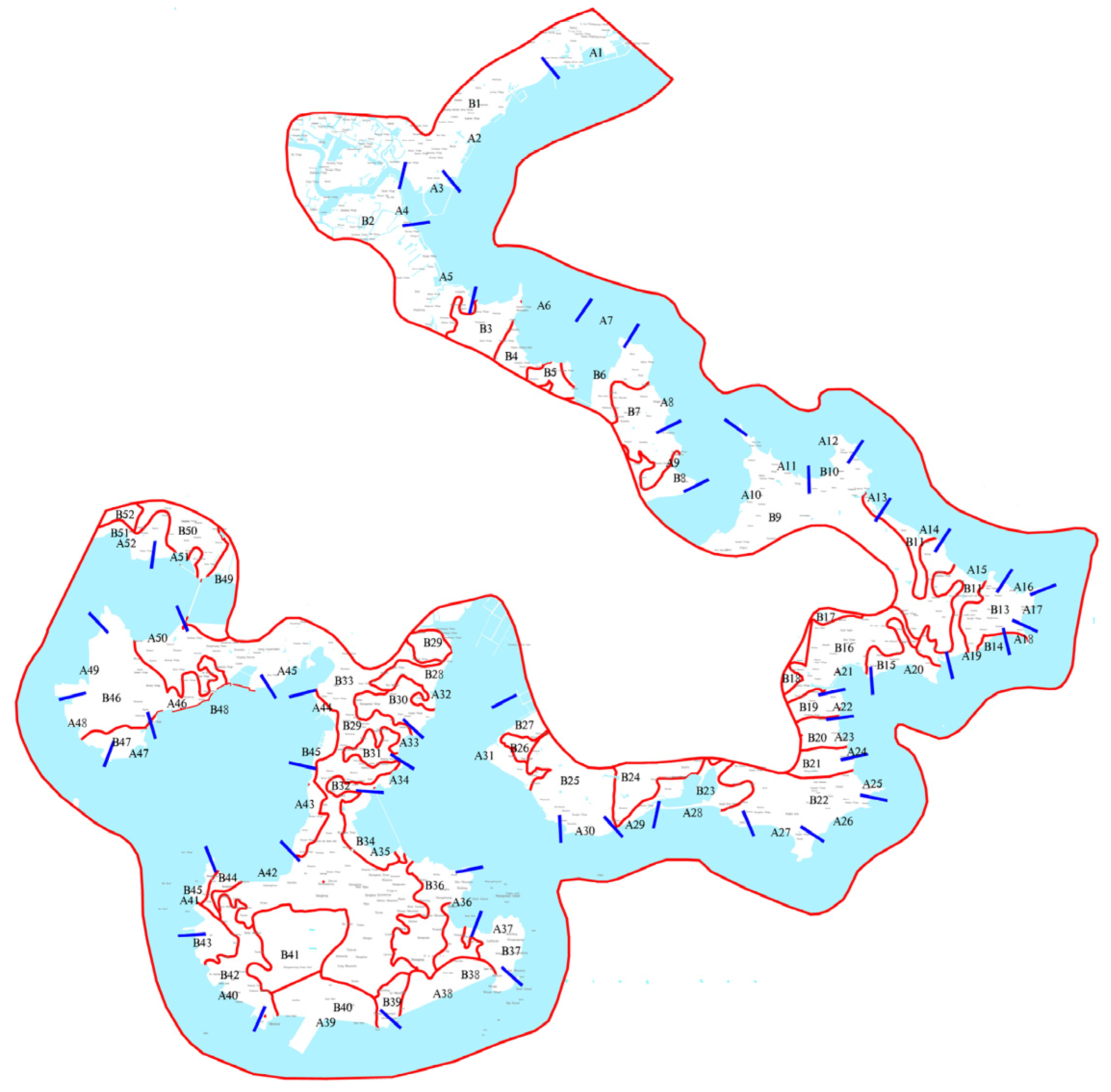
The coastal zone engineering in the study area is mainly based on the port, the port industry, and a suitability evaluation of coastal zone construction, namely, a suitability evaluation of port, wharf and pollution-prone industry and power plant construction [24,25]. From a comprehensive study of geological conditions for engineering and previous work experience, the coastal zone was divided into 52 evaluation units as shown in Figure 3, and we selected 20 typical units for the field investigation. On the basis of the principle of the simple and easy determination of influencing factors, 10 and 12 influencing factors were selected as evaluation indexes for port, wharf and pollution prone industry and power plants, respectively (refer to Appendix A, Table A1). Impact factor parameter values are shown in Table 1 and Table 2 (which list only 10 typical units): the qualitative indicators are based on expert ratings (due to textual limitations, the scoring criteria are not listed in detail). According to previous studies, the suitability of engineering construction is divided into four grades, namely good (I), better (II), poor (III) and bad (IV); for the classification criteria of each factor, refer to Appendix A, Table A2 and Table A3.
3.2. Determination of the Weight Coefficient of AHP
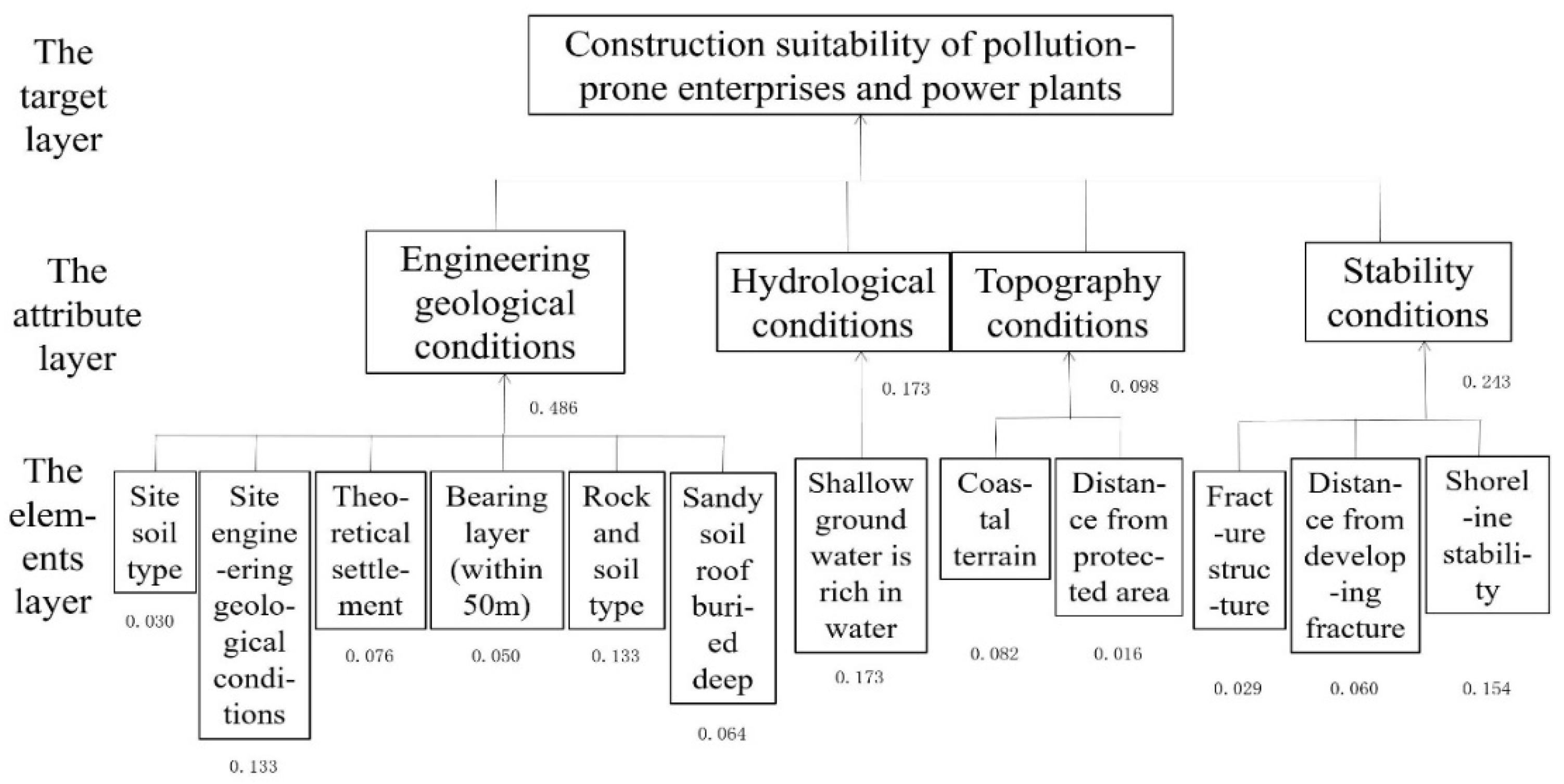
Through the analysis of geological factors for coastal engineering construction, the hierarchy structure model of the suitability evaluation of the port terminal, pollution-prone industry, and the power plant construction is constructed. The analytic hierarchy structure is divided into three layers—the object layer, the attribute layer, and the factor layer—calculated by the evaluation index weights, as shown in Figure 4 and Figure 5.
3.2.1. Raw Data Intensive Reduction
First, the consistency of the sample data was checked, and the results show that the 20 samples are compatible. Then, the attribute reduction was carried out according to the expression of the theory reduction process; the index factors could not be reduced, and all of them were kernels.
3.2.2. Calculate the Weight Coefficient of Each Index Factor
The collection of the typical areas of the evaluation system is regarded as the domain of information system U. According to the formula, the conditional attribute set C of the terminal and condition set B of the polluting enterprise and the power plant are respectively classified according to the conditional attributes and the decision attribute D, respectively:
For the positive field,
Among these,
The following is a classification of the domains after the removal of a conditional attribute:
3.2.3. Determination of the Weighting Factor
As calculated by the original data of the index factor,
The weight coefficient of the influence factor is
The weight factors X1, X2, ……X10 for port terminal evaluation are 0.041, 0.337, 0.048, 0.049, 0.017, 0.039, 0.032, 0.121, 0.018, and 0.298. The evaluation factor weight coefficients Y1, Y2, ……Y12 for pollution enterprises and power plants are 0.041, 0.121, 0.068, 0.049, 0.067, 0.059, 0.102, 0.091, 0.081, 0.055, 0.062, and 0.204.
3.3. Construct the Combination Weighting Judgment Evaluation Matrix
According to Theorem 1 [17], the combination judgment matrix is constructed, and the combination weighting value is calculated. We made a decision to meet the tendency of expert experience, i.e., to meet the . When the decision is to meet the tendency of objective data, . For decision making expert experience, we meet 0.5 ≤≤ 1, and when using objective decision making data, we meet . Here, is 0.38, and makes the subjective and objective matrix coefficients ratio the golden number; then, . By constructing the combination judgment matrix C, the weight coefficients of each index combination can be calculated, as shown in Table 3. X2, X10, Y4, and Y12 have a large combination weight coefficient, which indicates that the shore waters before width, site category, shoreline stability, fracture structure have a greater influence on the evaluation system. Special care should be taken for these factors in conducting the evaluation.
We can then use Equation (22) and Table 3 for the engineering construction suitability evaluation, according to the comprehensive evaluation of the adaptability zoning classification—good adaptability (level I, F ≥ 0.6), preferably adaptability (level II, 0.4 ≤ F < 0.6), poor adaptability (level III, 0.2 ≤ F < 0.4), and poor adaptability (level IV, F < 0.2)—and the actual construction suitability evaluation; comparison results are shown in Table 4 and Table 5, with visible evaluation results.
Among them, is the normalized value of the evaluation index, and is the combination weight coefficient.
3.4. Results of the Suitability Evaluation of Coastal Zone Engineering Construction Based on a Combined Weighted Judgment Matrix
Through the analysis of a typical coastal zone and a large-scale engineering survey, an engineering geological model, and information of engineering construction examples reflecting the current situation of engineering construction and affecting the dynamic environment, and considering the requirements of major coastal engineering ports, pollution-prone enterprises and power plants’ on-site conditions, 10 and 12 indicators were finally selected to be combined with the combined judgment matrix evaluation method for the comprehensive evaluation of coastal construction, as shown in Table 4 and Table 5. In this paper, the three-layer NNs model was constructed based on the impact factor indexes of Table 1 and Table 2 and the comprehensive evaluation of engineering construction suitability. The model is composed of 10 nodes and 12 nodes, and the outputs are four nodes. In total, 20 typical examples were used as learning samples of NNs. After learning convergence, 52 evaluation units of the coastal zone were predicted by using convergent network structure and parameters. The prediction results are shown in Table 6 and Table 7.
4. Discussion
4.1. Validation and Limitations of the RS-AHP-NNs Model
In order to verify the accuracy of the RS-AHP-NNs evaluation model, the raw data were processed using the AHP method alone (listing only 10 typical units). Finally, the predicted results of the AHP model, the predicted results of the RS-AHP-NNs model, and the actual results were compared, so as to verify the superiority and accuracy of the comprehensive evaluation model proposed in the article.
Based on the results calculated in Section 3.2, the AHP weighting factors were obtained. The results of the AHP evaluation of the suitability of engineering construction were obtained using Equation (23), and the comparison results are shown in Table 8.
Among them, is the normalized value of the evaluation index, and is the AHP weight coefficient.
From the above table, we can see that the predicted results of the RS-AHP-NNs integrated evaluation model and the actual engineering evaluation results are consistent. In contrast, the accuracy of the prediction results using the AHP analysis model alone is only 50%. The comparison of the three clearly shows that the RS-AHP-NNs comprehensive evaluation model is more consistent with the actual results, and is more accurate than the traditional AHP model. This indicates that the RS-AHP-NNs comprehensive evaluation model proposed in this paper can accurately reflect the actual situation of the suitability of coastal zone construction, and that it has some practical significance.
Although the RS-AHP-NNs comprehensive evaluation model analysis procedure provides an effective and convenient method, it is important to note that the model itself is still subject to some limitations. First, the resolution of impact factors is limited by the accuracy of the data measurement and grid generation. This means that the accuracy of the evaluation grid and measurement data can affect the authenticity and objectivity of the overall evaluation results. Secondly, the multi-level comparison in the RS-AHP-NNs model needs to give a comparison of its consistency. The method loses its usefulness if the consistency index requirement is not met during the hierarchical comparison.
4.2. Analysis Based on the RS-AHP-NN Model
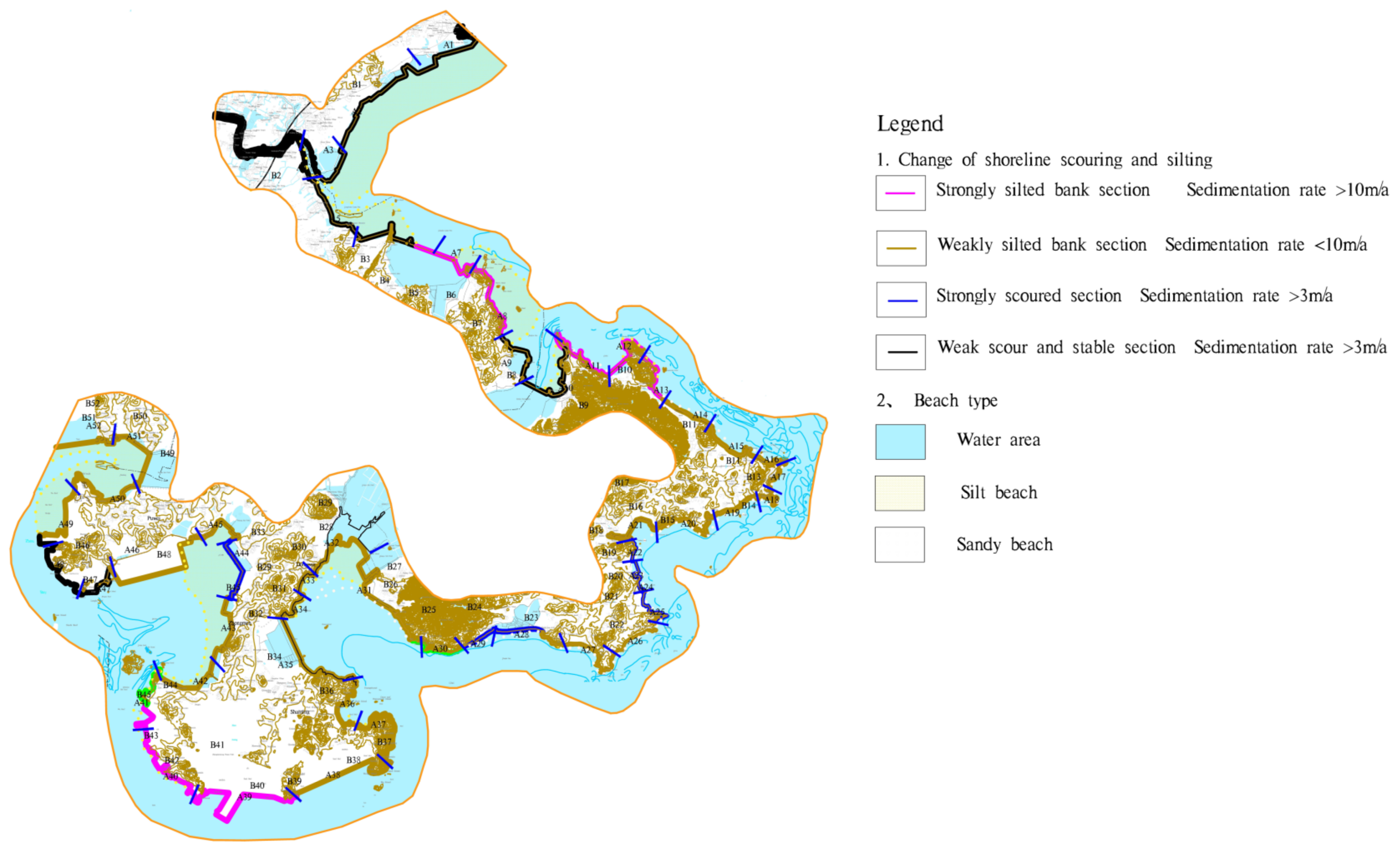
According to the comprehensive evaluation results of the RS-AHP-NN model, as can be seen from Table 6 and Figure 6, there are eights ections with good adaptability (level I), 19 sections in preferable condition (level II), 14 sections in poor condition (level III), and 11 sections in bad condition (level IV). The length and ratio of each shoreline are shown in Table 9. The evaluation results show that good or better locations belong to the bedrock or sandy areas along seashores, the scouring and silting in the shoreline change is not significant, there are no soft-soil or sandy-soil liquefaction phenomena, the coastal topography is flat and wide, and the width of the waterfront is wide, which is beneficial to the construction of the port terminal. The evaluation results show that the poor or poorer areas are mainly distributed in sandy or silty coast, have a shoreline deposition status, have a speed of 1–10 m/a, have groundwater salinity greater than 3 g/L, and have corrosion resistance in the building foundations; the thickness of the soft soil is great, and the buried depth of the roof is less than 5 m. It is easy to cause the seismic subsidence of soft soil, and the width of the intertidal zone is 1~2 km. This is not conducive to the construction of ship berthing and port terminal.
As can be seen from Table 7 and Figure 7, there are five zones with good adaptability (level I, preferable ones with 23 areas (level II), poor ones with four districts (level III) and 20 districts with bad areas (level IV) and ratios, as shown in Table 10. Among them, the area with the evaluation results of good or better belong to the flat and open terrain; moreover, the lithology is mainly intrusive rock and residual soil, the engineering geological condition is good, and the bearing capacity is high. The neural network evaluation structure is poor or bad, and the geological condition is usually a double-layer or multi-layer structure. The lithology is mainly composed of marine sediment, silty soil and sandy soil. The compressibility of the rock soil layer is higher, the bearing capacity is lower, and the groundwater level is shallow. It is easy to cause the uneven settlement of the foundation. The groundwater in the coastal section is salty water, and has strong corrosiveness.
5. Conclusions
(1) Based on the combination of a rough set and an analytical hierarchy process, a new evaluation method of a combined weighted judgment matrix was proposed. The RS-AHP-NN comprehensive evaluation model was used to analyze the contribution of each factor to the construction of the coastal zone, and the results are consistent with the actual survey results. The model was improved by introducing the combined judgment matrix and neural network to make the weights of the influencing factors more objective, which excluded the interference information and obtained the real and objective conclusion.
(2) In this paper, the engineering and geological conditions and previous work experience were studied comprehensively, and the coastal zone was divided into 52 evaluation units. According to the principle of simple and easy to implement impact factors, 10 and 12 impact factors of ports, docks and pollution-prone industries and power plants were selected as evaluation indexes, respectively. Based on the RS-AHP-NN coastal zone construction suitability analysis model, the weighting results of the impact factors were obtained. The weight factors X1, X2, ……X10 for port terminal evaluation were 0.057, 0.259, 0.059, 0.049, 0.062, 0.049, 0.086, 0.106, 0.017, and 0.256. The evaluation factor weight coefficients Y1, Y2, ……Y12 for pollution-prone enterprises and power plants were 0.048, 0.134, 0.064, 0.155, 0.063, 0.058, 0.070, 0.071, 0.034, 0.052, 0.045, and 0.206. Among them, the shore waters before the width, site category, shoreline stability, and fracture structure had a greater impact on the evaluation system.
(3) According to the validation, the RS-AHP-NNs comprehensive evaluation model had higher accuracy compared to the AHP evaluation model. The predicted results of the RS-AHP-NNs model were in full agreement with the actual findings, while the AHP model had only 50 percent accuracy. This shows that the comprehensive evaluation model proposed in this paper can reflect the real situation of the suitability of coastal zone construction, and it is a very effective method.
Author Contributions
Conceptualization, Y.L.; methodology, L.H. and Y.L.; formal analysis, Q.Z.; investigation, W.G.; data curation, Z.C.; writing—review and editing, T.M. All authors have read and agreed to the published version of the manuscript.
Funding
This research received no external funding.
Institutional Review Board Statement
Not applicable.
Informed Consent Statement
Not applicable.
Data Availability Statement
The manuscript data used to support the findings of this study are available from the corresponding author upon request.
Conflicts of Interest
The authors declare that they have no known competing financial interest or personal relationships that could have appeared to influence the work reported in this paper.
Appendix A
Table A1.
The referential relationship of the influence factors.
Table A1.
The referential relationship of the influence factors.
Character
Influence Factor
Character
Influence Factor
X1 (m)
channel depth
Y2 (m)
the theory of settlement
X2
shore waters before width
Y3
bearing layer
X3 (m)
shoreline stability
Y4 (m/a)
shoreline stability
X4 (m)
land for width
Y5
rock and soil types
X5
coastal zone type
Y6
sand roof depth
X6 (m)
undersea terrain
Y7 (m3/d)
shallow groundwater enrichment
X7 (m)
tidal range
Y8
the coastal terrain
X8 (m)
intertidal zone width
Y9 (m)
culture area of safe distance
X9
site engineering geological conditions
Y10 (m)
the seismogenic fault distance
X10
site category
Y11
site category
Y1
engineering conditions
Y12
fracture structure
Table A2.
Suitability classification standard of the port wharf.
Table A2.
Suitability classification standard of the port wharf.
Suitability Standard
X1 (m)
X2 (m)
X3
X4 (m)
X5
X6 (m)
X7 (m)
X8 (m)
X9
X10
good
≥10
≥426
8
≥2000
8
≤5
≤4.8
≤200
8
8
better
[5, 10)
[324, 426]
6
[1000, 2000)
6
[5, 10)
[4.8, 5)
[200, 500)
6
6
poor
[3, 5)
[200, 324)
4
[500, 1000)
4
[10, 15)
[5, 5.2)
500, 1000
4
4
bad
<3
<200
2
<500
2
>15
>5.2
>1000
2
2
Table A3.
Suitability classification standard of pollution-prone industry and power plants.
Table A3.
Suitability classification standard of pollution-prone industry and power plants.
Suitability Standard
Y1
Y2 (m)
Y3
Y4 (m/a)
Y5
Y6
Y7 (m3/d)
Y8
Y9 (m)
Y10 (m)
Y11
Y12
good
8
≤0.1
8
≤5
8
8
≤10
4
≥1000
≥1000
4
4
better
6
(0.1, 0.3]
6
(5, 10]
6
6
(10, 100]
3
[500, 1000)
[500, 1000)
3
3
poor
4
(0.3, 0.5]
4
(10, 30]
4
4
(100, 1000]
2
[200, 500)
[300, 500)
2
2
bad
2
>0.5
2
>30
2
2
>1000
1
<200
<300
1
1
References
Fan, X.Z.; Yuan, L.; Dai, X.Y.; Zhang, L.Q. The integrated coastal zone management (ICZM) and its progress. Acta Ecol. Sin.2010, 10, 2756–2765. [Google Scholar]
Xue, X.Z.; Hong, H.S.; Charles, A.T. Cumulative environmental impacts and integrated coastal management: The case of Xiamen, China. J. Environ. Manag.2004, 71, 271–281. [Google Scholar] [CrossRef] [PubMed]
Tie, Y.B.; Tang, C.; Zhou, C.H. The application of AHP to emergency response capability assessment in urban disaster. J. Geol. Hazards Environ. Preserv.2005, 43, 45–53. [Google Scholar]
Yang, S.R.; Ding, S. A method for bridge damage identification and evaluation based on strain ratio. J. Highw. Transp. Res. Dev.2021, 38, 87–96. [Google Scholar]
Gong, Y. The environmental monitoring data statistical analysis and evaluation of chongqing steel environmental air quality. CISC Technol.2018, 61, 54–57. [Google Scholar]
Negash, B.M. Artificial neural network based production forecasting for a hydrocarbon reservoir under water injection. Pet. Explor. Dev.2020, 47, 357–365. [Google Scholar]
Chen, Y. Construction engineering quality evaluation model based on genetic algorithm. Mod. Electron. Tech.2020, 43, 126–128. [Google Scholar]
Qi, J.K. Research on comprehensive evaluation model of engineering safety of large pumping station based on genetic algorithm. Heilongjiang Hydraul. Sci. Technol.2020, 48, 39–42. [Google Scholar]
Chen, Z.F.; Wu, J.; Guo, Y.B.; Lin, T. Application of AHP and fuzzy mathematics in comprehensive assessment of mine environment. East China Geol.2018, 39, 305–310. [Google Scholar]
Liang, J.; Zhou, L.T.; Liu, Z.K. Hazard assessment of concrete dam fracture based on the improved cloud-evidence theory. J. Shandong Agric. Univ. (Nat. Sci. Ed.)2020, 51, 547–552. [Google Scholar]
Wang, Z.W.; Li, D.Y.; Wang, X.G. Application of evidence right method in landslide risk zonation. Chin. J. Geotech. Eng.2007, 29, 1268–1273. [Google Scholar]
Xie, Q.H.; Zhang, X.W.; Lv, W.G.; Cheng, S.Y. Public Transport Scheme Optimized by Election Campaign Algorithm and Extension Theory. Adv. Intell. Syst. Res.2016, 130, 143–147. [Google Scholar]
Ma, M.; Qu, X. Risk Evaluation of Gas Pipeline Based on Rough Set. Appl. Mech. Mater.2014, 443, 256–258. [Google Scholar]
Liu, M.; Shao, M.; Zhang, W.; Wu, C. Reduction method for concept lattices based on rough set theory and its application. Comput. Math. Appl.2007, 53, 1390–1410. [Google Scholar] [CrossRef] [Green Version]
Song, X.X. Rough sets theory and its applications. J. Xianyang Norm. Univ.2005, 20, 29–31. [Google Scholar]
Pan, M.M.; Huang, T.; Xiao, Z.X. Analysis of the analysis of the influence factors of the influence factors of the water inflow in the tunnel of the tunnel. J. Hydraul. Archit. Eng.2010, 8, 132–134. [Google Scholar]
Sun, Q.; Zhang, T.L.; Wu, J.B.; Wang, H.S. Landslide risk assessment of the Longxi river basin based on GIS and AHP. East China Geol.2018, 39, 227–233. [Google Scholar]
Galushkin, A.I. Neural Network Theory; Springer: New York, NY, USA, 2007. [Google Scholar]
Wang, M.W.; Luo, G.Y.; Zhang, G. Application of neural network to regional stability evaluation of Yang Qiao bridge project. Geol. Explor.2001, 37, 80–82. [Google Scholar]
Zhang, J.L. Application of BP neural network. J. Shijiazhuang Vocat. Technol. Inst.2015, 27, 34–36. [Google Scholar]
Xiang, M.S.; Chen, J.; Liu, R. Assessment of the Bridge Technical State Based on the BP Neural Network. Transp. Sci. Technol.2011, 5, 547–552. [Google Scholar]
Peng, K.; Chen, L. Evaluation of County New Urbanization Quality Based on BP Neural Network. J. Jialing Univ.2017, 35, 42–46. [Google Scholar]
Deakin, M.; Reid, A. Sustainable urban development: Use of the environmental assessment methods. Sustain. Cities Soc.2014, 10, 39–48. [Google Scholar] [CrossRef]
Tong, J.; Chai, B. Geological environment risk assessment for residential land and public facilities land at Caofeidain newly-developed areas. J. Eng. Geol.2013, 21, 501–507. [Google Scholar]
Figure 1.
Putian location information map.
Figure 1.
Putian location information map.
Figure 2.
Configuration of the BP network.
Figure 2.
Configuration of the BP network.
Figure 3.
The coast is divided into 52 evaluation units.
Figure 3.
The coast is divided into 52 evaluation units.
Figure 4.
Suitability evaluation index hierarchy model of port wharf engineering construction.
Figure 4.
Suitability evaluation index hierarchy model of port wharf engineering construction.
Figure 5.
Suitability evaluation index hierarchy model of pollution-prone industrial and power plant engineering construction.
Figure 5.
Suitability evaluation index hierarchy model of pollution-prone industrial and power plant engineering construction.
Figure 6.
Suitability evaluation diagram for the engineering construction of a port wharf.
Figure 6.
Suitability evaluation diagram for the engineering construction of a port wharf.
Figure 7.
Suitability evaluation map of pollution-prone enterprises and power plant construction.
Figure 7.
Suitability evaluation map of pollution-prone enterprises and power plant construction.
Table 1.
Each influence factor index of the port wharf.
Table 1.
Each influence factor index of the port wharf.
Evaluation Units
X1 (m)
X2 (m)
X3
X4 (m)
X5
X6 (m)
X7 (m)
X8 (m)
X9
X10
A1
2.5
216
4
498
2
15.7
4.6
1100
4
4
A3
3
220
4
510
2
14.5
4.6
1000
4
4
A8
4.5
310
4
820
4
11.2
4.7
810
4
4
A9
7
412
6
1700
6
4.7
4.6
420
6
6
A13
7.2
420
6
1680
6
4.5
4.6
413
6
6
A14
11
458
8
2100
6
4.1
4.5
198
8
8
A16
4.3
321
4
837
4
10.3
4.7
823
4
4
A20
4.4
331
4
790
4
7.6
4.6
795
4
4
A22
3.4
321
4
498
4
10.3
4.6
578
4
6
A25
11.3
473
8
2300
8
3.8
4.6
157
8
8
Table 2.
Each influence factor index of pollution-prone industries and power plants.
Table 2.
Each influence factor index of pollution-prone industries and power plants.
Evaluation Units
Y1
Y2 (m)
Y3
Y4 (m/a)
Y5
Y6
Y7 (m3/d)
Y8
Y9 (m)
Y10(m)
Y11
Y12
A1
2
0.6
2
32.2
2
2
600
1
180
267
1
3
A3
6
0.2
6
8.2
6
6
70
3
750
860
3
3
A8
6
0.3
6
3.1
6
6
78
3
800
970
3
3
A9
8
0.1
8
3.3
8
8
13
4
1200
1100
4
3
A13
2
0.8
2
34.1
2
4
700
2
400
260
1
3
A14
6
0.2
6
6.3
6
4
86
3
660
800
3
3
A16
6
0.1
6
7.2
6
6
90
3
700
900
3
3
A20
6
0.2
6
8.1
4
4
86
3
680
850
3
3
A22
2
0.7
2
34.5
2
4
750
1
450
280
1
3
A25
6
0.2
6
5.7
6
6
80
3
860
900
3
3
Table 3.
Each factor of the combination empowerment value.
Table 3.
Each factor of the combination empowerment value.
Impact Factor
Combination Weight Coefficient
X1
0.057
X2
0.259
X3
0.059
X4
0.049
X5
0.062
X6
0.049
X7
0.086
X8
0.106
X9
0.017
X10
0.256
Y1
0.048
Y2
0.134
Y3
0.064
Y4
0.155
Y5
0.063
Y6
0.058
Y7
0.070
Y8
0.071
Y9
0.034
Y10
0.052
Y11
0.045
Y12
0.206
Table 4.
Suitability evaluation grades of port wharf engineering construction.
Table 4.
Suitability evaluation grades of port wharf engineering construction.
Evaluation Unit
Comprehensive Score F
Order of Suitability Evaluation
Actual Grade
A1
0.113
IV
IV
A3
0.121
IV
IV
A8
0.273
III
III
A9
0.457
II
II
A13
0.428
II
II
A14
0.611
I
I
A16
0.334
III
III
A20
0.291
III
III
A22
0.273
III
III
A25
0.753
I
I
A27
0.476
II
II
A28
0.490
II
II
A31
0.540
II
II
A32
0.143
IV
IV
A34
0.284
III
III
A36
0.346
III
III
A40
0.419
II
II
A43
0.524
II
II
A44
0.653
I
I
A48
0.878
I
I
Table 5.
Suitability evaluation grades of pollution-prone industrial and power plant engineering construction.
Table 5.
Suitability evaluation grades of pollution-prone industrial and power plant engineering construction.
Evaluation Unit
Comprehensive Score F
Order of Suitability Evaluation
Actual Grade
B1
0.123
IV
IV
B3
0.433
II
II
B8
0.587
II
II
B9
0.649
I
I
B13
0.046
IV
IV
B14
0.484
II
II
B16
0.467
II
II
B20
0.362
II
II
B22
0.079
IV
IV
B25
0.488
II
II
B27
0.210
III
III
B28
0.438
II
II
B31
0.468
II
II
B32
0.683
I
I
B34
0.457
II
II
B36
0.565
II
II
B40
0.473
II
II
B43
0.154
IV
IV
B44
0.431
II
II
B48
0.631
I
I
Table 6.
Suitability neural network evaluation results of port wharf engineering construction.
Table 6.
Suitability neural network evaluation results of port wharf engineering construction.
Evaluation Unit
Suitability Level
Evaluation Unit
Suitability Level
Evaluation Unit
Suitability Level
Evaluation Unit
Suitability Level
A1
IV
A14
I
A27
II
A40
II
A2
IV
A15
II
A28
II
A41
II
A3
IV
A16
III
A29
IV
A42
II
A4
IV
A17
II
A30
III
A43
II
A5
IV
A18
II
A31
II
A44
I
A6
IV
A19
II
A32
IV
A45
II
A7
IV
A20
III
A33
III
A46
III
A8
III
A21
III
A34
III
A47
I
A9
II
A22
III
A35
III
A48
I
A10
IV
A23
I
A36
III
A49
II
A11
IV
A24
I
A37
II
A50
II
A12
II
A25
I
A38
III
A51
III
A13
II
A26
II
A39
II
A52
III
Table 7.
Suitability neural network evaluation results of pollution-prone industrial and power plant engineering construction.
Table 7.
Suitability neural network evaluation results of pollution-prone industrial and power plant engineering construction.
Evaluation Unit
Suitability Level
Evaluation Unit
Suitability Level
Evaluation Unit
Suitability Level
Evaluation Unit
Suitability Level
B1
IV
B14
II
B27
III
B40
II
B2
IV
B15
II
B28
II
B41
IV
B3
II
B16
II
B29
II
B42
I
B4
IV
B17
II
B30
II
B43
IV
B5
II
B18
I
B31
II
B44
II
B6
IV
B19
II
B32
I
B45
I
B7
II
B20
II
B33
II
B46
II
B8
II
B21
II
B34
II
B47
IV
B9
I
B22
IV
B35
IV
B48
I
B10
IV
B23
IV
B36
II
B49
IV
B11
IV
B24
II
B37
I
B50
I
B12
IV
B25
II
B38
IV
B51
IV
B13
IV
B26
II
B39
II
B52
II
Table 8.
Comparison of the AHP and RS-AHP-NNs evaluation results.
Table 8.
Comparison of the AHP and RS-AHP-NNs evaluation results.
Evaluation Unit
Grade of AHP Evaluation
Grade of RS-AHP-NNs Evaluation
Actual Grade
A1
IV
IV
IV
A3
III
IV
IV
A8
III
III
III
A9
III
II
II
A13
III
II
II
A14
III
I
I
A16
III
III
III
A20
III
III
III
A22
III
III
III
A25
III
I
I
Table 9.
Suitability of the coastline length and its percentage of port wharf.
Table 9.
Suitability of the coastline length and its percentage of port wharf.
Suitability Level
Good (I)
Preferably (II)
Poor (III)
Bad (IV)
Length (km)
24.5
97.9
70.4
67.7
Percentage
9.4%
37.6%
27%
26%
Table 10.
Suitability of the coastline length and its percentage of pollution-prone industrial and power plant engineering construction.
Table 10.
Suitability of the coastline length and its percentage of pollution-prone industrial and power plant engineering construction.
Suitability Level
Good (I)
Preferably (II)
Poor (III)
Bad (IV)
Area (km2)
59.7
130.7
13.5
164.7
Percentage
16.2%
35.5%
3.7%
44.6%
Publisher’s Note: MDPI stays neutral with regard to jurisdictional claims in published maps and institutional affiliations.
Li, Y.; Hou, L.; Zhang, Q.; Ge, W.; Chen, Z.; Meng, T.
Evaluation of Coastal Zone Construction Based on Theories of the Combination of Empowerment Judgment and Neural Networks: The Example of the Putian Coastal Zone. Symmetry2022, 14, 1028.
https://0-doi-org.brum.beds.ac.uk/10.3390/sym14051028
AMA Style
Li Y, Hou L, Zhang Q, Ge W, Chen Z, Meng T.
Evaluation of Coastal Zone Construction Based on Theories of the Combination of Empowerment Judgment and Neural Networks: The Example of the Putian Coastal Zone. Symmetry. 2022; 14(5):1028.
https://0-doi-org.brum.beds.ac.uk/10.3390/sym14051028
Chicago/Turabian Style
Li, Yunfeng, Lili Hou, Qing Zhang, Weiya Ge, Zongfang Chen, and Tianyu Meng.
2022. "Evaluation of Coastal Zone Construction Based on Theories of the Combination of Empowerment Judgment and Neural Networks: The Example of the Putian Coastal Zone" Symmetry 14, no. 5: 1028.
https://0-doi-org.brum.beds.ac.uk/10.3390/sym14051028
Note that from the first issue of 2016, this journal uses article numbers instead of page numbers. See further details here.
Article Metrics
No
No
Article Access Statistics
For more information on the journal statistics, click here.
Multiple requests from the same IP address are counted as one view.
Li, Y.; Hou, L.; Zhang, Q.; Ge, W.; Chen, Z.; Meng, T.
Evaluation of Coastal Zone Construction Based on Theories of the Combination of Empowerment Judgment and Neural Networks: The Example of the Putian Coastal Zone. Symmetry2022, 14, 1028.
https://0-doi-org.brum.beds.ac.uk/10.3390/sym14051028
AMA Style
Li Y, Hou L, Zhang Q, Ge W, Chen Z, Meng T.
Evaluation of Coastal Zone Construction Based on Theories of the Combination of Empowerment Judgment and Neural Networks: The Example of the Putian Coastal Zone. Symmetry. 2022; 14(5):1028.
https://0-doi-org.brum.beds.ac.uk/10.3390/sym14051028
Chicago/Turabian Style
Li, Yunfeng, Lili Hou, Qing Zhang, Weiya Ge, Zongfang Chen, and Tianyu Meng.
2022. "Evaluation of Coastal Zone Construction Based on Theories of the Combination of Empowerment Judgment and Neural Networks: The Example of the Putian Coastal Zone" Symmetry 14, no. 5: 1028.
https://0-doi-org.brum.beds.ac.uk/10.3390/sym14051028
Note that from the first issue of 2016, this journal uses article numbers instead of page numbers. See further details here.


