
Topological Study of 6.82 D Carbon Allotrope Structure

School of Advanced Sciences, Vellore Institute of Technology University, Vellore 632014, Tamilnadu, India
*
Author to whom correspondence should be addressed.
Symmetry 2022, 14(5), 1037; https://0-doi-org.brum.beds.ac.uk/10.3390/sym14051037
Submission received: 4 April 2022
/
Revised: 5 May 2022
/
Accepted: 13 May 2022
/
Published: 18 May 2022
(This article belongs to the Section Mathematics)
Abstract
:Carbonallotropes are widely available and can be found in the atmosphere, the earth’s crust, and in living creatures in myriad forms. Allotropes are also used in several fields, including for medicinal and biological applications, due to their intriguing properties such as low resistance, high electron mobility, abnormal quantum hall effect, unconventional superconductivity in graphene, and so on. The theoretical analysis of carbon allotropes can hence be quite useful as it leads to a better understanding of the nature and behavior of these ubiquitous materials and also opens the door for even better applications. The objective of this research is to theoretically analyze the carbon allotrope by using four kinds of vertex degree based (VDB) topological indices (Tis), namely VDB multiplicative topological indices, VDB indices using M-Polynomial, VDB entropy measures, and irregularity indices. This analysis will extend the current body of knowledge available for this allotrope and help future researchers in the synthesis of new allotropes.
1. Introduction
Mathematical chemistry is a subfield of theoretical chemistry that uses graph theory to analyze molecule structure. In other words, it ensures the properties of the chemistry of this structure by specifying the vertices, edges, and degree vertices graph of the molecular structure using mathematical methods. Many chemistry problems can be solved using these strategies. The theory of chemical graphs is a branch of mathematical chemistry; in fact, graph theory connects chemistry with mathematics, and it uses graph theory to answer many of mathematical chemistry’s most challenging issues. The topologic index, also known as a connection index, characterizes the chemical makeup of a substance based on its molecular structure [1,2,3].
Tis of massive chemical structures, such as metal organic frameworks, can be particularly valuable in both characterization and computing physicochemical parameters that are difficult to compute for such vast networks in reticular chemistry [4,5,6]. In recent years, the synthesis of innovative reticular metal-organic frameworks and networks in which covalent fibers are braided into crystals has become more essential. Topological indices are numerical representations of molecule structural properties produced by the application of graph-theoretical principles to vast networks of interest in mystifying chemistry. Several degree-based indices have been developed to test the properties of compounds and drugs, and they are widely used in chemical and pharmacy engineering. Topological indices can be thought of as a collection of parameters on a molecular graph. This is crucial in theoretical physics and pharmacology science.
Carbon is a relatively common element that can be found in the atmosphere, the universe’s core, and living things in many forms. Under ambient conditions, carbon’s capacity to form sp, sp2, and sp3hybridised bonds results in the formation of diverse allotropes [7].Carbon atoms form a flat sheet known as graphene when they have no curve, while a positive curvature generates the soccer ball-like structure known as buckyballs. For decades, scientists have hypothesized that a third variety—a structure with negative curvature—should exist. In this study we discussed about one of the typical negatively curved carbon allotrope named as carbon allotrope structure [8].
6.82 D Carbon Allotrope
The carbon allotrope structure is typical negatively curved carbon allotrope and it can be obtained by the condensation of truncated-icosahedral C60 molecules. Twelve atoms, or six “double” bonds, are taken away from each C60 molecule in such a way that the remaining 48atoms, arranged as eight hexagons, maintain cubic symmetry. The truncated structure, thus obtained, is joined to six similar structures along the six cubic face directions, resulting in four eight sided rings at each juncture. This process results in an allotrope which has been predicted to possess remarkable stability, approximately 0.23 eV/atom more stable than C60. In relative terms, the smallest molecular fullerene known to have the same relative energy has 180 carbon atoms [7,9,10,11]. The carbon allotrope was also predicted to be an insulator. The spongy structure of the allotrope, that is, the large ordered hollows, could host alkali metal ions, similar to naturally occurring zeolite structures. In 2012, Szeflerand Diudea represented the structure in graph-theoretical terms, using the Omega polynomial [12,13,14,15]. The relatively high stability of this structure, as well as its numerous possible applications, prompted this study to conduct a structural theoretical examination of the allotrope. The structure is investigated at the molecular level in this article utilizing vertex degree based (VDB) and related indices.
There are currently no studies in the literature that look at this structure from a topological perspective. As a result, this research is unique, and it will contribute to a deeper knowledge of the allotrope as well as more precise predictions of its physical and chemical properties. The findings in this paper could be used to comparable allotropes that are designed and synthesized in the future. The basic mathematical terminology were covered in Section 2 of this article. The methodology was discussed in Section 3. VDB multiplicative Tis, VDB indices utilizing M-polynomial, VDB entropy measures, and VDB irregularity indices for the 6.82 Carbon Allotrope are computed in part 4 using edge-partitioning techniques. Section 6 concludes the paper by doing numerical analysis on the computed data.
2. Mathematical Terminologies
In this paper, represents a connected graph, and refer to the vertex set and the edge set, respectively. The degree of a vertex in a graph is the number of edges that are adjacent to that vertex [16]. We used edge-partition approaches to generate VDB Multiplicative Tis, VDB indices utilizing M-polynomial, VDB entropy measures, and VDB irregularity indices for the Carbon Allotrope.
2.1. Multiplicative Topological Indices
Some multiplicative topological indices have been researched in recent years, for example, in [17,18]. In Nano carbon Kwun et al. they computed the Multiplicative Degree-Based Topological Indices of Silicon-Carbon Si2C3-I[p,q] and Si2C3-II[p,q] [19].Yousaf, S.A. et al. discussed Carbon Nanotubes using degree based Tis [20].
The multiplicative topological index [21] is represented as
where denotes the product of the terms . The multiplicative version of the Wiener index was the first topological index investigated [22].
The first multiplicative hyper-Zagreb index is described [25] as
The multiplicative Harmonic index of a graph is defined as
Multiplicative ABC index, multiplicative GA index, and are defined as
and
The multiplicative augmented Zagreb index is defined as
2.2. VDB Indices Utilising M-Polynomial
There are currently many algebraic polynomials available in the literature that can be used to calculate distance-based Tis. Among them, the Hosoya polynomial has been the most widely employed, since several distance-based indices can be computed using a single polynomial. In 2015, Deutsch and Klavžar [28] made a similar breakthrough for VDB indices in the form of M-polynomial. Similar to the Hosaya polynomial, the M-polynomial can also be used in the computation of several VDB indices. JulietrajaandVenugopal studied the topological descriptors of coronoid systems and Benzenoid systems using M-polynomials [29,30]. Farkhanda et al., introduced some new degree based topological indices via M polynomial [31]. Rauf, A. et al., computed an algebraic polynomial based topological study of graphite carbon nitride (g–) molecular structure [32]. Guangyu, L. et al., carried out an analysis of carbon nanotube and polycyclic aromatic nanostar molecular structures [33].
The M-polynomial of is defined as
where and is the edge for which . Table 1 shows that the M-polynomial Topological Indices.
, ,
, , , , , , , .
2.3. VDB Entropy Measures for 6.82 Carbon Allotrope
Let be the order of a graph of size and is some meaningful information function. The Shannons entropy [34] of a graph is depicted as
Let and the degree of is represented by the information function that is, . Then the Equation (1) can be rewritten as
The fundamental theorem of graph theory is represented as . As a result, the above equation becomes
Chen et al. [35] introduced the entropy measure of an edge-weighted graph. If is an edge-weighted graph, where and represents vertex set, edge set and the edge weight of the edge of , then we have:
The Equations (1)–(3) are used to calculate the following entropy measures which are listed below in Table 2.
2.4. IrregularityIndices for 6.82 Carbon Allotrope
Irregularity indices are a quantitative measure of the irregularity of a graph. An irregularity index is a numerical quantity if it is non-zero for an irregular graph and becomes zero for a regular graph. The first index of this kind was proposed by Bell in [36]. The measure of irregularity of a molecular can be applied to a variety of open topics, including material chemistry and engineering. In QSPR investigations, the VDB irregularity index has been used to predict physical and chemical properties such as acentric factor (Acen Fac), entropy, standard enthalpy of vaporisation (DHVAP), and other significant chemical properties [37].Juliet Raja et al. studied the topology of the benzenoid system using distance-based descriptors. This paper mainly focuses on computing the degree-based and irregularity-based descriptors for Benzenoid systems [38,39]. Table 3 shows that the Irregularity based topological indices.
3. Methods
Graph theoretical approaches, the edge partition method, and analytical techniques are used in this study to complete the computations. Analytical expressions for the degree-based M-Polynomial, entropy measurements, and irregularity indices based on analytical expressions are all obtained using Maple. Chem Draw Ultra is used to describe the molecular structures of Carbon Allotrope, while Origin is used to visualize numerical findings.
4. Main Results
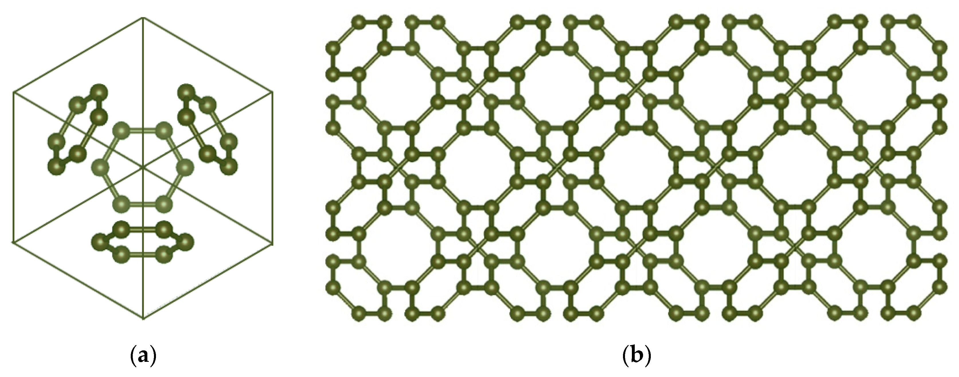
We give our most important findings in this part, which is separated into Four subcategories. Figure 1a illustrates 6.82 D 3D molecular graph. We used the following settings to characterize its molecular graph: The number of connected unit cells in a row (chain) is represented by , and the number of connected rows with number of cells is represented by . We demonstrated how cells join in a row (chain) and how one row relates to another in Figure 1b.The total number of vertices and edges of is depicted as and . In addition, there are three edge partitions in the edge set. Edges are contained in the first edge partition are , where . The second edge partition is made up of edges, and . Edges are contained in the thirdedge partitionare , where . The edge partition of the Structure is shown in below Table 4.
4.1. Numerical Aspects of 6.82 D Carbon Allotrope Structure: VDB Multiplicative Topological Indices
Theorem 1.
IfCarbon Allotrope, then the VDB multiplicative TIs are computed as
- (i)
- (ii)
- (iii)
- (iv)
- (v)
- (vi)
- (vii)
- (viii)
- (ix)
Proof.
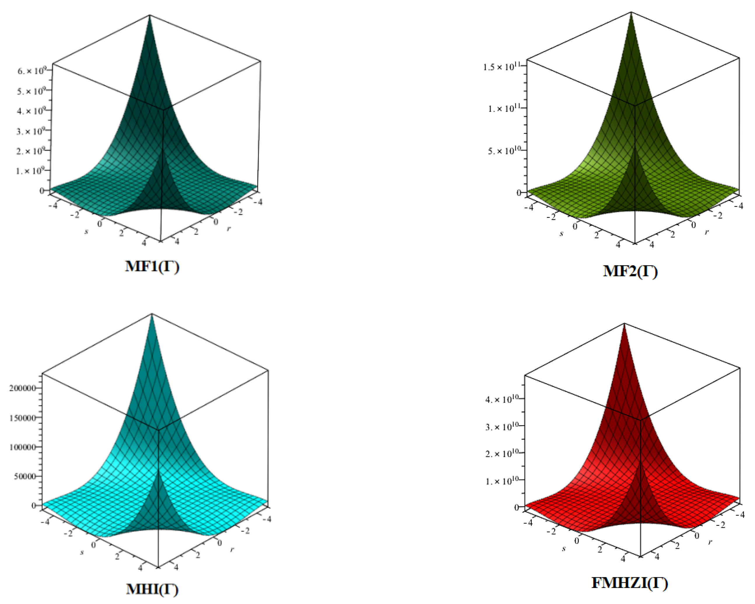
Let be a Carbon Allotrope. The total number of vertices and edges of is depicted as and . By using the definitions of VDB multiplicative TIs and the Edge partition, the following results are obtained as follows and Figure 2 shows the 3D plots of the Results.
- (i)
- (ii)
- (iii)
- (iv)
- (v)
- (vi)
- (vii)
- (viii)
- (ix)
Hence the proof. □

4.2. Numerical Aspects of 6.82 D Carbon Allotrope Structure: M-Polynomial Topological Indices
Theorem 2.
If Carbon Allotrope, then the M-polynomial is computed as
Proof.
Using the definition of M-polynomial and Table 1, the following result is obtained as
Hence the proof. □
Theorem 3.
If Carbon Allotrope, then the VDB indices using M-polynomial are computed as
Proof.
- ABC index
- GA index
- The first K-Banhatti index
- The second K-Banhatti index
- The first K-hyper Banhatti index
- The second K-hyper Banhatti index,,
- The Modified first K-Banhatti index,
- The Modified second K-Banhatti index,
- The Harmonic K-Banhatti index,
Hence the proof. □
4.3. Numerical Aspects of 6.82 D Carbon Allotrope Structure: Degree Based Entropy Measures
For this proof, we will utilize Table 2.
First Zagrebentropy
Second Zagreb entropy
Second modified Zagreb entropy
Reduced second Zagreb entropy
Hyper Zagreb entropy
The augmented Zagreb entropy
Atom bond connectivity entropy
Geometric arithmetic entropy
First redefined Zagreb entropy
Second redefined Zagreb entropy
Third redefined Zagreb entropy
The symmetric division deg (SDD) entropy
Arithmetic-geometric entropy
The forgotten entropy
Sum-connectivity entropy
4.4. Numerical Aspects of 6.82 D Carbon Allotrope Structure: Irregularity Indices for 6.82 Carbon Allotrope
Theorem 4.
IfCarbon Allotrope, then the irregularity-based indices are computed as
Proof.
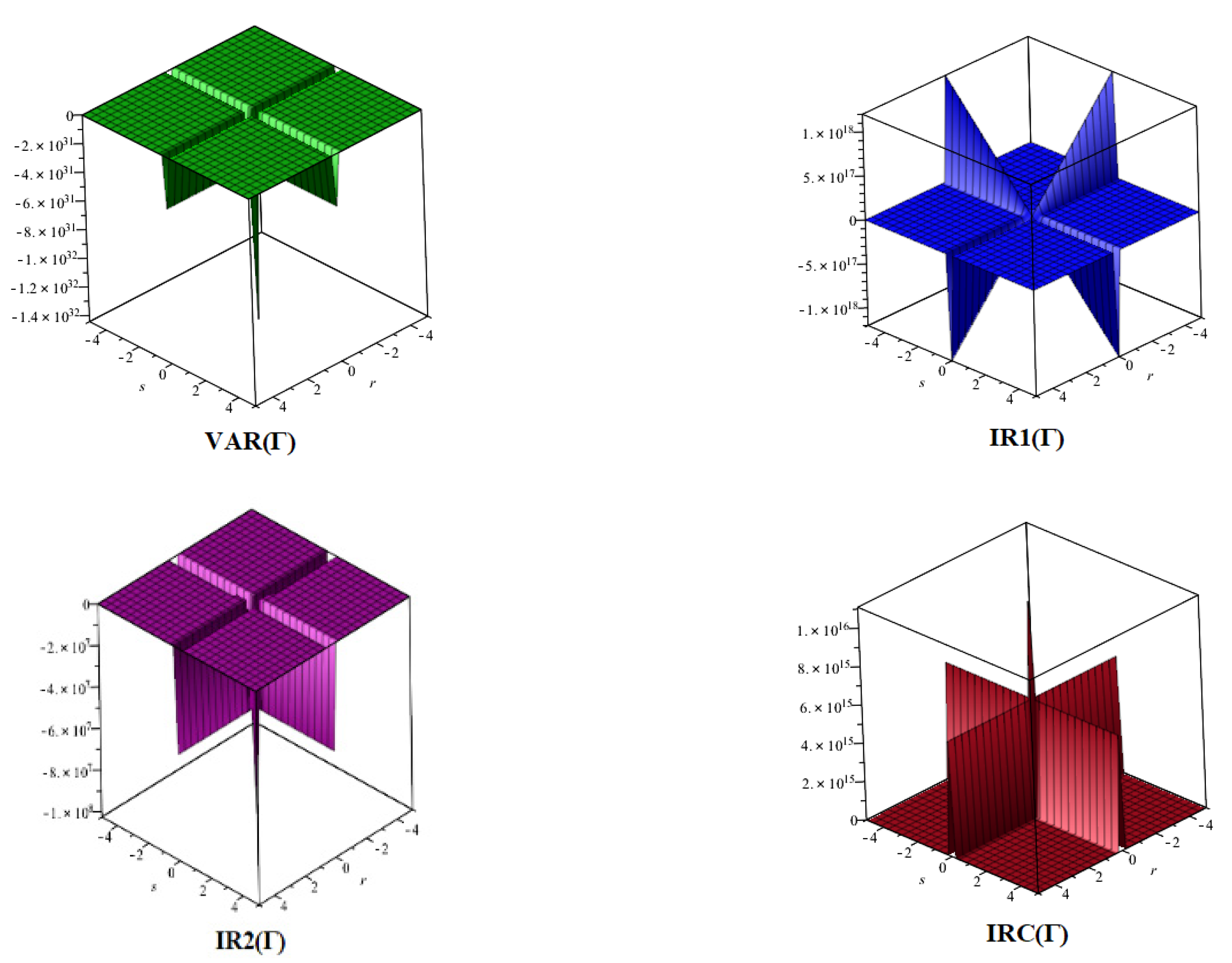
Let be a carbon allotrope. The cardinality of carbon allotrope is depicted as and . Using the definitions of irregularity-based indices and the Table 3, we get the following result as and Figure 4 shows the 3D plots of the Results.
Hence the proof. □
Figure 4.
3D plots for in Theorem 4.

5. Numerical Results
6. Conclusions
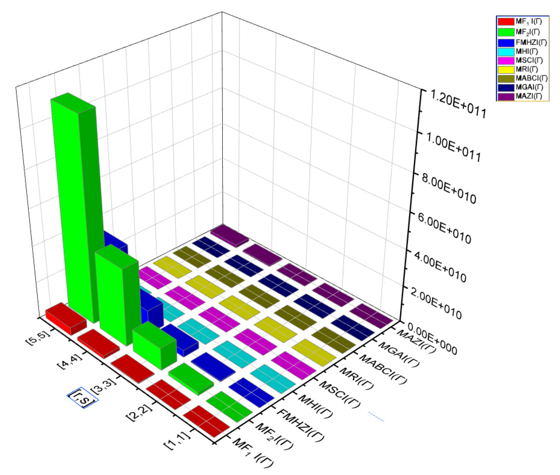
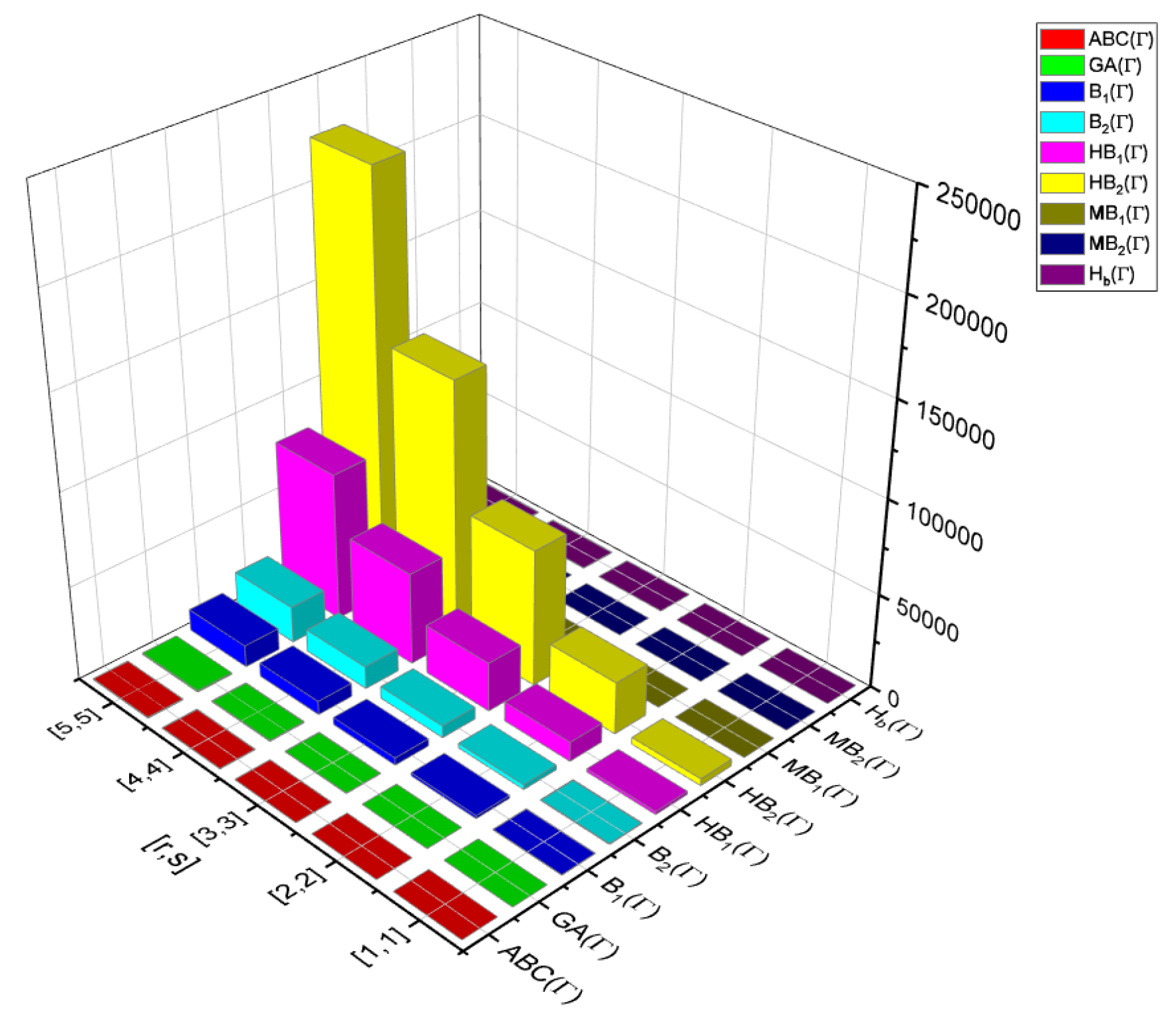
In this article, the closed expressions for VDB indices, irregularity indices, and VDB entropy measures have been computed using M-polynomial and edge-partition techniques. We have performed numerical comparisons for Multiplicative and M-polynomial topological indices, as well as irregularity and entropy metrics. Figure 5 shows that dominates the other indices among Multiplicative TIs, while Figure 6 shows that dominates the other indices among M-Polynomial TIs. In general, the 6.8 structure has the best heat conductivity property with impressive stability, a close theoretical analysis of this structure will lay the groundwork to design newer allotropes with the desired features based on the computed VDB indices.
Negatively curved carbon is difficult to visualize since, instead of bending outwards like a sphere, it bends inwards like a saddle. It has been extremely difficult to synthesize these negatively-curved carbons on their own. Due to their ability to transport high amounts of electrical charge, these carbons could be used in a variety of applications, including improved capacitors, in which the biological activity or other qualities of molecules are connected with their chemical structure, are one application of topological indices. It will give the different perspective to the researchers.
Author Contributions
L.R.M.G. contributes for conceptualization, software, methodology and writing original draft. D.G. contributes for supervision, validation, formal analysis, review and editing. All authors have read and agreed to the published version of the manuscript.
Funding
The research work is supported by Vellore Institute of Technology, Vellore-632014.
Institutional Review Board Statement
Not applicable.
Informed Consent Statement
Not applicable.
Data Availability Statement
Not applicable.
Acknowledgments
The authors wish to thank the management of Vellore Institute of Technology, Vellore-632014, for their continuous support and encouragement to carry out this research work.
Conflicts of Interest
The authors declare no conflict of interest.
References
- West, D.B. Introduction to Graph Theory; Prentice Hall: Upper Saddle River, NJ, USA, 2001. [Google Scholar]
- Mihalić, Z.; Trinajstić, N. A Graph-Theoretical Approach to Structure-Property Relationships. J. Chem. Educ. 1992, 69, 701. [Google Scholar] [CrossRef] [Green Version]
- Gutman, I.; Rušci´c, B.; Trinajsti´c, N.; Wilcox, C.F. Graph theory and molecular orbitals, XII. Acyclic polyenes. J. Chem. Phys. 1975, 62, 3399–3405. [Google Scholar] [CrossRef]
- Siddiqui, M.K.; Imran, M.; Ahmad, A. On Zagreb indices, Zagreb polynomials of some nanostardendrimers. Appl. Math. Comput. 2016, 280, 132–139. [Google Scholar] [CrossRef]
- García, I.; Fall, Y.; Gómez, G. Using Topological Indices to Predict Anti-Alzheimer and Anti-Parasitic GSK-3 Inhibitors by Multi-Target QSAR in Silico Screening. Molecules 2010, 15, 5408–5422. [Google Scholar] [CrossRef]
- Basak, S.C.; Mills, D.; Mumtaz, M.M.; Balasubramanian, K. Use of Topological Indices in Predicting Aryl Hydrocarbon Re-ceptor Binding Potency of Dibenzofurans: A Hierarchical QSAR Approach; IJC-A; NISCAIR-CSIR: New Delhi, India, 2003; Volume 42A, pp. 1385–1391. Available online: http://nopr.niscair.res.in/handle/123456789/20670 (accessed on 3 April 2022).
- Feng, X.; Mu, H.; Xiang, Z.; Cai, Y. Theoretical Investigation of Negatively Curved 6.82D Carbon Based on Density Functional Theory. Comput. Mater. Sci. 2020, 171, 109211. [Google Scholar] [CrossRef]
- Felix, L.C.; Woellner, C.F.; Galvao, D.S. Mechanical and Energy-Absorption Properties of Schwarzites. Carbon 2020, 157, 670–680. [Google Scholar] [CrossRef] [Green Version]
- Gibson, J.; Holohan, M.; Riley, H.L. Amorphous Carbon. J. Chem. Soc. 1946, 456–461. [Google Scholar] [CrossRef]
- Sabirov, D.S.; Ori, O.; Tukhbatullina, A.A.; Shepelevich, I.S. Covalently Bonded Fullerene Nano-Aggregates (C60)n: Digitalizing Their Energy-Topology-Symmetry. Symmetry 2021, 13, 1899. [Google Scholar] [CrossRef]
- Sabirov, D.S.; Ori, O. Skeletal Rearrangements of the C240 Fullerene: Efficient Topological Descriptors for Monitoring Stone-Wales Transformations. Mathematics 2020, 8, 968. [Google Scholar] [CrossRef]
- O’Keeffe, M.; Adams, G.B.; Sankey, O.F. Predicted New Low Energy Forms of Carbon. Phys. Rev. Lett. 1992, 68, 2325–2328. [Google Scholar] [CrossRef]
- Barborini, E.; Piseri, P.; Milani, P.; Benedek, G.; Ducati, C.; Robertson, J. Negatively Curved Spongy Carbon. Appl. Phys. Lett. 2002, 81, 3359–3361. [Google Scholar] [CrossRef]
- Baerlocher, C.; Mccusker, L.B.; Olson, B.; Meier, W.M.; Ebrary, I. Atlas of Zeolite Framework Types; Elsevier: Boston, MA, USA; Amsterdam, The Netherlands, 2007. [Google Scholar]
- Hoffmann, R.; Kabanov, A.A.; Golov, A.A.; Proserpio, D.M. Homo Citans and Carbon Allotropes: For an Ethics of Citation. Angew. Chem. Int. Ed. 2016, 55, 10962–10976. [Google Scholar] [CrossRef] [PubMed]
- West, D.B. Introduction to Graph Theory; Pearson Prentice Hall: Upper Saddle River, NJ, USA, 2018; (revised April 2018). [Google Scholar]
- Gutman, I.; Milovanovic, I.; Milovanovic, E. Relations between Ordinary and Multiplicative Degree-Based Topological Indices. Filomat 2018, 32, 3031–3042. [Google Scholar] [CrossRef] [Green Version]
- Hussain, Z.; Ijaz, N.; Tahir, W.; Butt, M.T.; Talib, S. Calculating Degree Based Multiplicative Topological Indices of Alcohol. SSRN Electron. J. 2018. [Google Scholar] [CrossRef]
- Jahanbani, A.; Shao, Z.; Sheikholeslami, S.M. Calculating Degree Based Multiplicative Topological Indices of Hyaluronic Acid-Paclitaxel Conjugates’ Molecular Structure in Cancer Treatment. J. Biomol. Struct. Dyn. 2020, 39, 5304–5313. [Google Scholar] [CrossRef]
- Kwun, Y.C.; Virk, A.U.R.; Nazeer, W.; Rehman, M.A.; Kang, S.M. On the Multiplicative Degree-Based Topological Indices of Silicon-Carbon Si2C3-I[P,Q] and Si2C3-II[P,Q]. Symmetry 2018, 10, 320. [Google Scholar] [CrossRef] [Green Version]
- Yousaf, S.; Bhatti, A.A.; Aslam, A. Study of Carbon Nanbotubes and Boron Nanotubes Using Degree Based Topological Indices. Polycycl. Aromat. Compd. 2021, 1–14. [Google Scholar] [CrossRef]
- Todeschini, R.; Consonni, V. New Local Vertex Invariants and Molecular Descriptors Based on Functions of the Vertex Degrees. MATCH Commun. Math. Comput. Chem. 2010, 64, 359–372. [Google Scholar]
- Das, K.C.; Gutman, I. On Wiener and Multiplicative Wiener Indices of Graphs. Discret. Appl. Math. 2016, 206, 9–14. [Google Scholar] [CrossRef]
- Sarkar, P.; De, N.; Pal, A. Correction to: On Some Multiplicative Version Topological Indices of Block Shift and Hierarchical Hypercube Networks. OPSEARCH 2021. [Google Scholar] [CrossRef]
- Todeschini, R.; Consonni, V. Handbook of Molecular Descriptors; Wiley-VCH: Weinheim, Germany, 2000. [Google Scholar]
- Kulli, V.R. Multiplicative hyper-Zagreb indices and coindices of graphs: Computing these indices of some nanostructures. Int. Res. J. Pure Algebra 2016, 6, 342–347. [Google Scholar]
- Gutman, I.; Furtula, B.; Katanić, V. Randić Index and Information. AKCE Int. J. Graphs Comb. 2018, 15, 307–312. [Google Scholar] [CrossRef]
- Kulli, V.R. General Multiplicative Zagreb Indices of TUC4C8[M,N] and TUC4[M,N] Nanotubes. Int. J. Fuzzy Math. Arch. 2016, 11, 39–43. [Google Scholar] [CrossRef]
- Deutsch, E.; Klavžar, S. M-Polynomial Revisited: Bethe Cacti and an Extension of Gutman’s Approach. J. Appl. Math. Comput. 2018, 60, 253–264. [Google Scholar] [CrossRef] [Green Version]
- Julietraja, K.; Venugopal, P.; Prabhu, S.; Liu, J.-B. M-Polynomial and Degree-Based Molecular Descriptors of Certain Classes of Benzenoid Systems. Polycycl. Aromat. Compd. 2021, 1–30. [Google Scholar] [CrossRef]
- Julietraja, K.; Venugopal, P. Computation of Degree-Based Topological Descriptors Using M-Polynomial for Coronoid Systems. Polycycl. Aromat. Compd. 2020, 1–24. [Google Scholar] [CrossRef]
- Afzal, F.; Hussain, S.; Afzal, D.; Razaq, S. Some New Degree Based Topological Indices via M-Polynomial. J. Inf. Optim. Sci. 2020, 41, 1061–1076. [Google Scholar] [CrossRef]
- Rauf, A.; Ishtiaq, M.; Muhammad, M.H.; Siddiqui, M.K.; Rubbab, Q. Algebraic Polynomial Based Topological Study of Graphite Carbon Nitride (G-) Molecular Structure. Polycycl. Aromat. Compd. 2021, 1–22. [Google Scholar] [CrossRef]
- Guangyu, L.; Hussain, S.; Khalid, A.; Ishtiaq, M.; Siddiqui, M.K.; Cancan, M.; Imran, M. Topological Study of Carbon Nanotube and Polycyclic Aromatic Nanostar Molecular Structures. Polycycl. Aromat. Compd. 2021, 1–21. [Google Scholar] [CrossRef]
- Shannon, C.E. A Mathematical Theory of Communication. Bell Syst. Tech. J. 1948, 27, 379–423. [Google Scholar] [CrossRef] [Green Version]
- Chen, Z.; Dehmer, M.; Shi, Y. A Note on Distance-Based Graph Entropies. Entropy 2014, 16, 5416–5427. [Google Scholar] [CrossRef]
- Réti, T.; Tóth-Laufer, E. On the Construction and Comparison of Graph Irregularity Indices. Kragujev. J. Sci. 2017, 39, 53–75. [Google Scholar] [CrossRef] [Green Version]
- Réti, T.; Tóth-Laufer, E. Graph Irregularity Indices Used as Molecular Descriptors in QSPR Studies. MATCH Commun. Math. Comput. Chem. 2018, 79, 509–524. [Google Scholar]
- Chu, Y.-M.; Julietraja, K.; Venugopal, P.; Siddiqui, M.K.; Prabhu, S. Degree- and Irregularity-Based Molecular Descriptors for Benzenoid Systems. Eur. Phys. J. Plus 2021, 136, 78. [Google Scholar] [CrossRef]
Figure 1.
(a) The unit cell of 6.82 D. (b) View from the top of a 6.82 D super cell.

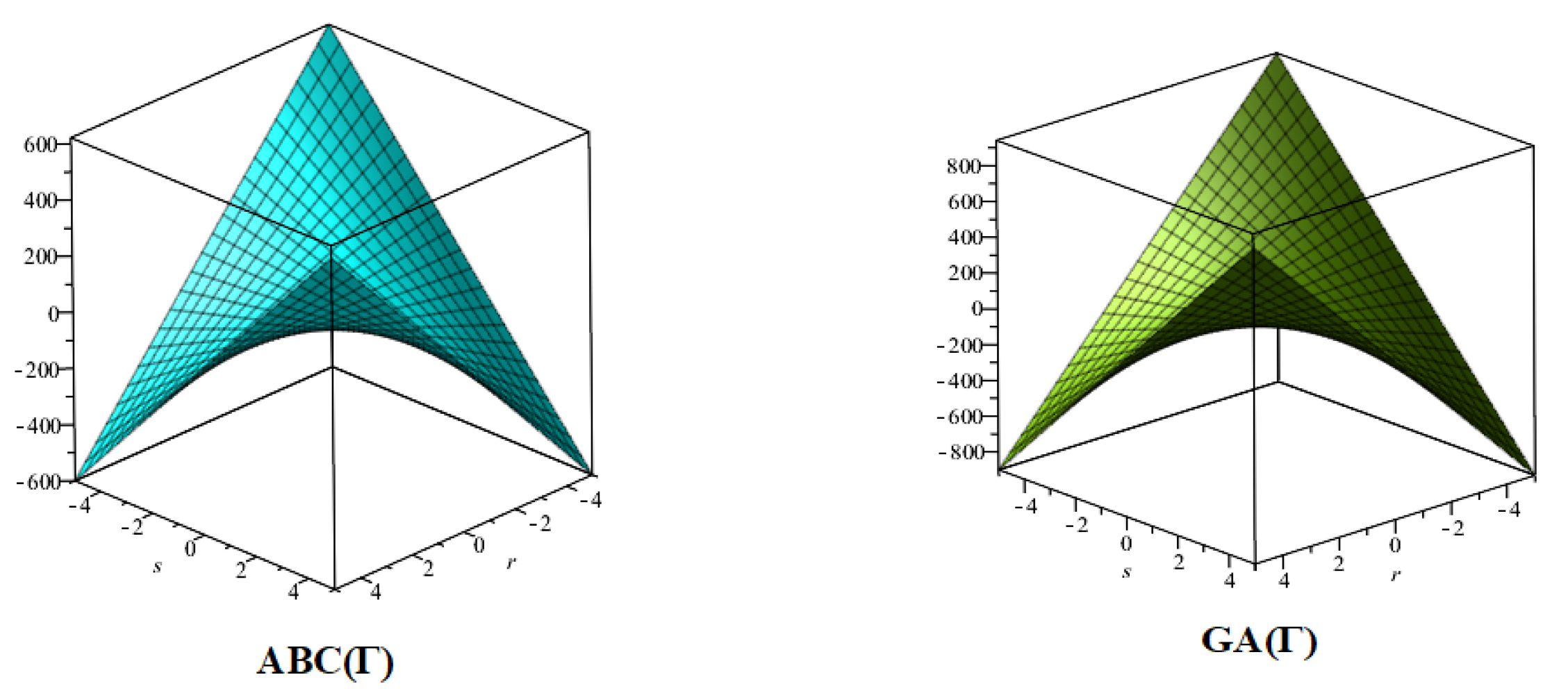
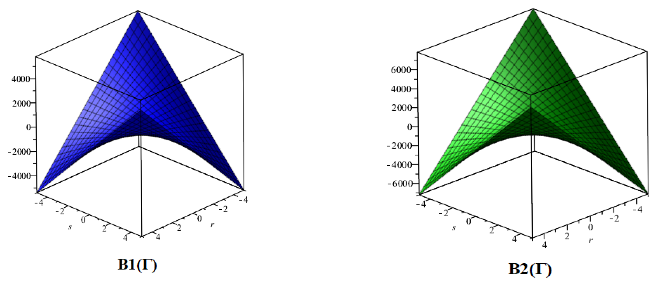
Figure 3.
3D plots for in Theorem 3.


Figure 5.
The comparison of multiplicative topological indices for 6.82 D carbon allotrope.

Figure 6.
The comparison ofM-polynomial topological indices for 6.82 D Carbon allotrope.


Table 1.
Degree based M-polynomials.
| S. No | |
|---|---|
| 1 | |
| 2 | |
| 3 | |
| 4 | |
| 5 | |
| 6 | |
| 7 | |
| 8 | |
| 9 |
Table 2.
Edge weight and VDB entropy.
| S. No | Degree Based Entropy | Mathematical Expressions |
|---|---|---|
| 1 | First Zagreb entropy | |
| 2 | Second Zagreb entropy | |
| 3 | Second modified Zagreb entropy | |
| 4 | Reduced second Zagreb entropy | |
| 5 | Hyper Zagreb entropy | |
| 6 | Augmented Zagreb entropy | |
| 7 | Atom bond connectivity entropy | |
| 8 | Geometric arithmetic entropy | |
| 9 | First redefined Zagreb entropy | |
| 10 | Second redefined Zagreb entropy | |
| 11 | Third redefined Zagreb entropy | |
| 12 | Symmetric division deg (SDD) entropy | |
| 13 | Arithmetic- geometric entropy | |
| 14 | Forgotten entropy | |
| 15 | Sum-connectivity entropy |
Table 3.
VDB irregularity indices.
| S. No | Mathematical Expressions |
|---|---|
| 1 | |
| 2 | |
| 3 | |
| 4 | |
| 5 | |
| 6 | |
| 7 | |
| 8 | |
| 9 | |
| 10 | |
| 11 | |
| 12 | |
| 13 | |
| 14 | |
| 15 |
Table 4.
Edge partition table of .
| Total Number of Edges | |
|---|---|
Table 5.
The computed VDB multiplicative topological indices of Theorem 1 are computed numerically in Table 5.
Table 5.
The computed VDB multiplicative topological indices of Theorem 1 are computed numerically in Table 5.
| [r,s] | |||||||||
|---|---|---|---|---|---|---|---|---|---|
| [1,1] | 1,437,696 | 35,831,808 | 11,059,200 | 51.0 | 70.110 | 52.2564 | 256.002 | 752.46 | 559,872 |
| [2,2] | 75,479,040 | 1,881,169,920 | 580,608,000 | 2677.5 | 3680.775 | 2743.4610 | 13,440.105 | 39,504.15 | 29,393,280 |
| [3,3] | 486,420,480 | 12,123,095,040 | 3,741,696,000 | 17,255.0 | 23,720.550 | 17,680.0820 | 86,614.010 | 25,458.23 | 189,423,360 |
| [4,4] | 1,705,826,304 | 42,514,440,192 | 13,121,740,800 | 60,511.5 | 83,185.515 | 62,002.2186 | 30,374.64 | 89,279.38 | 664,288,128 |
| [5,5] | 4,412,289,024 | 109,967,818,752 | 33,940,684,800 | 156,519 | 21,516.76 | 16,037.51 | 78,567.01 | 230,929.74 | 1,718,247,168 |
Table 6.
The M-polynomial topological indices of Theorem 2 are computed numerically in Table 6.
Table 6.
The M-polynomial topological indices of Theorem 2 are computed numerically in Table 6.
| [r,s] | |||||||||
|---|---|---|---|---|---|---|---|---|---|
| [1,1] | 19.475 | 27.838 | 296 | 408 | 1656 | 3624 | 11.219 | 9.5556 | 22.076 |
| [2,2] | 87.112 | 127.52 | 1600 | 2536 | 10336 | 27640 | 42.8 | 30.667 | 84.876 |
| [3,3] | 202.75 | 299.19 | 3912 | 6392 | 26072 | 72392 | 94.952 | 63.778 | 188.82 |
| [4,4] | 366.38 | 542.87 | 7232 | 11976 | 48864 | 137880 | 167.68 | 108.89 | 333.9 |
| [5,5] | 578.02 | 858.55 | 11560 | 19288 | 78712 | 224104 | 260.97 | 166 | 520.13 |
Publisher’s Note: MDPI stays neutral with regard to jurisdictional claims in published maps and institutional affiliations. |
© 2022 by the authors. Licensee MDPI, Basel, Switzerland. This article is an open access article distributed under the terms and conditions of the Creative Commons Attribution (CC BY) license (https://creativecommons.org/licenses/by/4.0/).
Share and Cite
MDPI and ACS Style
Gnanaraj, L.R.M.; Ganesan, D. Topological Study of 6.82 D Carbon Allotrope Structure. Symmetry 2022, 14, 1037. https://0-doi-org.brum.beds.ac.uk/10.3390/sym14051037
AMA Style
Gnanaraj LRM, Ganesan D. Topological Study of 6.82 D Carbon Allotrope Structure. Symmetry. 2022; 14(5):1037. https://0-doi-org.brum.beds.ac.uk/10.3390/sym14051037
Chicago/Turabian StyleGnanaraj, Leena Rosalind Mary, and Deepa Ganesan. 2022. "Topological Study of 6.82 D Carbon Allotrope Structure" Symmetry 14, no. 5: 1037. https://0-doi-org.brum.beds.ac.uk/10.3390/sym14051037
Note that from the first issue of 2016, this journal uses article numbers instead of page numbers. See further details here.