
A Method for Solving Approximate Partition Boundaries of Spatial Big Data Based on Histogram Bucket Sampling


1
Information Science and Technology College, Dalian Maritime University, Dalian 116026, China
2
Dalian Key Laboratory of Intelligent Software, Dalian 116026, China
*
Author to whom correspondence should be addressed.
Symmetry 2022, 14(5), 1055; https://0-doi-org.brum.beds.ac.uk/10.3390/sym14051055
Submission received: 2 May 2022
/
Revised: 13 May 2022
/
Accepted: 19 May 2022
/
Published: 20 May 2022
Abstract
:In recent years, the volume of spatial data has rapidly grown, so it is crucial to process them in an efficient manner. The level of parallel processing in big data platforms such as Hadoop and Spark is determined by partitioning the dataset. A common approach is to split the data into chunks based on the number of bytes. While this approach works well for text-based batch processing, in many cases, it is preferable to take advantage of the structured information contained in the dataset (e.g., spatial coordinates) to plan data partitioning. In view of the huge amount of data and the impossibility of quickly establishing partitions, this paper designs a method for approximate partition boundary solving, which divides the data space into multiple non-overlapping symmetric bins and samples each bin, making the probability density of the sampling set bounded by the deviation of the probability density of the original data. The sampling set is read into the memory at one time for calculation, and the established partition boundary satisfies the partition threshold-setting. Only a few boundary adjustment operations are required, which greatly shortens the partition time. In this paper, the method proposed in the paper is tested on the synthetic dataset, the bus trajectory dataset, and six common spatial partitioning methods (Grid, Z-curve, H-curve, STR, Kd-tree, and R*-Grove) are selected for comparison. The results show that the symmetric bin sampling method can describe the spatial data distribution well and can be directly used for partition boundary division.
1. Introduction
In recent years, the amount of spatial data generated by Internet of Things (IoT) sensors, social networks, and moving vehicles has significantly increased, which has led to many research efforts to develop processing frameworks that can handle spatial big data, e.g., JD Urban Spatio-Temporal (JUST) [1], Spatial In-Memory Big data Analytics (Simba) [2], SpatialHadoop [3] and others [4]. Regardless of their internal structure, all these systems have a common and necessary first step: spatial data partitioning. These systems partition data across machines and then process the partitions in parallel to scale out. Research shows that spatial data partitioning methods are critical to the performance of many spatial operations, such as load balancing, indexing, visualization, spatial join query, and k-NN join query.
In the MapReduce computing paradigm, partitioning a dataset into independent partitions is a critical operation, as the degree of parallelism and overall performance directly depends on the initial partitioning technique [3]. The basis of the MapReduce computing paradigm is to divide the input dataset into fixed-size chunks or slices, and execute the same map task in parallel on the chunks. If all map tasks can be executed in parallel, the total execution time depends on which map task takes longer. Therefore, when the map tasks are well balanced, the fastest parallel execution speed can be obtained. This means that dividing the data into chunks is the key to obtaining a well-balanced map task and ensuring faster execution. Common partitioning methods include hash partitioning, range partitioning and random partitioning [5]. Hash partitioning and random partitioning do not consider the content of the data; in the batch case the dataset is always analyzed in its entirety, so this solution is reasonable. However, this approach is not efficient if the dataset is analyzed using selective queries based on some attributes of the data (such as the spatial extent of the region). Range partitioning requires a predefined set of key ranges. However, in the big data environment, there is no set of key range statistics on the dataset, so it is challenging to solve the partition boundary in a low-cost and accurate way.
Data skew usually comes from the physical properties of objects (e.g., the height of a person follows a normal distribution) and hotspots in the spatial domain (e.g., urban structure spatial information follows a skewed distribution). The efficiency of these partitioning techniques depends on the characteristics and distribution of the dataset, so choosing an appropriate spatial partitioning technique for skewed data is an extremely challenging problem [3,6]. The main difficulty in building partitions is to quickly find the optimal size of each partition boundary to balance the amount of data that the partitions contain.
Obtaining precise partition boundaries requires calculating spatial datapoint locations and quantitative relationships. Although the MapReduce computing paradigm can analyze and process data in parallel, the huge amount of data cannot be read into memory for calculation at one time, and frequent I/O operations will greatly affect the speed of data partitioning; for example, the synthetic dataset is 3.26 GB in size and contains 100 million datapoints, and it takes 47 min to calculate its precise partition boundaries. The existing solution is to use sampling methods to randomly select small samples from the input data to represent the overall distribution of the data, e.g., SpatialHadoop [3] and SATO (Sample Analyze Tear Optimize) [7]. The processing step is to select a sample subset from the dataset based on a given sampling rate of . Then, the partition boundaries are obtained according to the data distribution of the subsets. Finally, the entire input records are scanned in parallel, and each record is allocated to a partition according to the spatial information of the record and the partition boundary. If the partition capacity exceeds the expected size and the partition boundary does not cover the datapoints, the partition boundary is adjusted. Random sampling can approximate the data distribution. However, the overall distribution description in the worst case cannot be guaranteed, resulting in excessive partition boundary adjustment operations, especially in the case of data skew and data hotspots. Aiming to solve the above problems, we propose an approximate partition boundary solution method based on histogram bucket sampling. In the sampling process, fully considering the data distribution characteristics, a sampling set with higher availability can be obtained, to more effectively perform fast partitioning for spatial big data. The main contributions of this paper are summarized as follows:
- A general sampling method is proposed for partition boundary solutions.
- A partition boundary calculation method based on histogram bucket sampling is proposed, and the rationality of this sampling method is proved. At the same time, a framework for the approximate estimation of histogram bucket size is proposed.
- The effectiveness of the proposed method is evaluated using six partitioning techniques on synthetic and real datasets. Compared with solutions based on random sampling, the proposed scheme can obtain approximate true partition boundaries.
The rest of this article is organized as follows. Section 2 shows the related research, Section 3 introduces histogram bucket sampling, in Section 4 we evaluate the effectiveness of the histogram bucket sampling method on synthetic and real datasets and, finally, the paper is summarized in Section 5.
2. Related Work
This section reviews the related work of solving the partition boundary of spatial big data. Partitioning is a basic operation for managing and processing big data on a cluster in a distributed system, and sampling is a necessary step for spatial big data partitioning operations [8]. When considering uniformly, spatially distributed data, spatial partitioning can be easily achieved using uniform random sampling over the entire spatial distribution to obtain the distribution of the input dataset; conversely, for skewed datasets, this may not be the right choice, and other sampling techniques must be applied [9]. Existing sampling techniques are mainly based on the expansion of statistical sampling [10,11]. Spatial Hadoop experiments with random sampling [12] on seven spatial partitioning techniques. Although the sampling time is about two minutes, due to the large number of unsampled points, a lot of partition boundary adjustment is required, so the fixed overhead of each map task in the MapReduce job is increased, and the efficiency is not high, especially in the case of data skew. ST-Hadoop [6] uses random sampling to estimate the spatial distribution of objects and how this distribution evolves over time, ST-Hadoop uses MapReduce to scan all data records to read samples, set the sampling rate to and the maximum size to 100MB, sort the samples in chronological order, and, within each time instance in the sample, amplify the size and number of data records associated with each time instance by . Kollios et al. [13] proposed a bias sampling technique based on local probability density. The local density function of each point is defined by the kernel function to calculate the sampling probability of each partition. Through the parameter , the sampling of uniformly distributed data or skewed distribution data can be realized; where dense or sparse regions are oversampled in skewed distribution data, this method facilitates clustering and outlier detection in large datasets. Yan et al. [14] proposed an error-bounded stratified sampling method to reduce data: by using buckets to cover data, the sampling rate of a small bucket value range is reduced, and the sampling rate of a large bucket value range is larger. This technology has a better performance when it is used for approximate query [15,16], and retains the characteristics of data aggregation, but there are two problems when using data partitioning: (1) The probability of scattered data being collected becomes low, the partition coverage rate is low, and a large number of partition boundary adjustment operations are generated; (2) The bucket sizes are different. If the skew of the dataset is large, some bucket sampling may have the same problem as Spatial Hadoop. To minimize data movement, Harsh et al. [17] use sampling and histogram-based techniques to partition keys, which combine sampling and iterative histograms to find high-quality partitions.
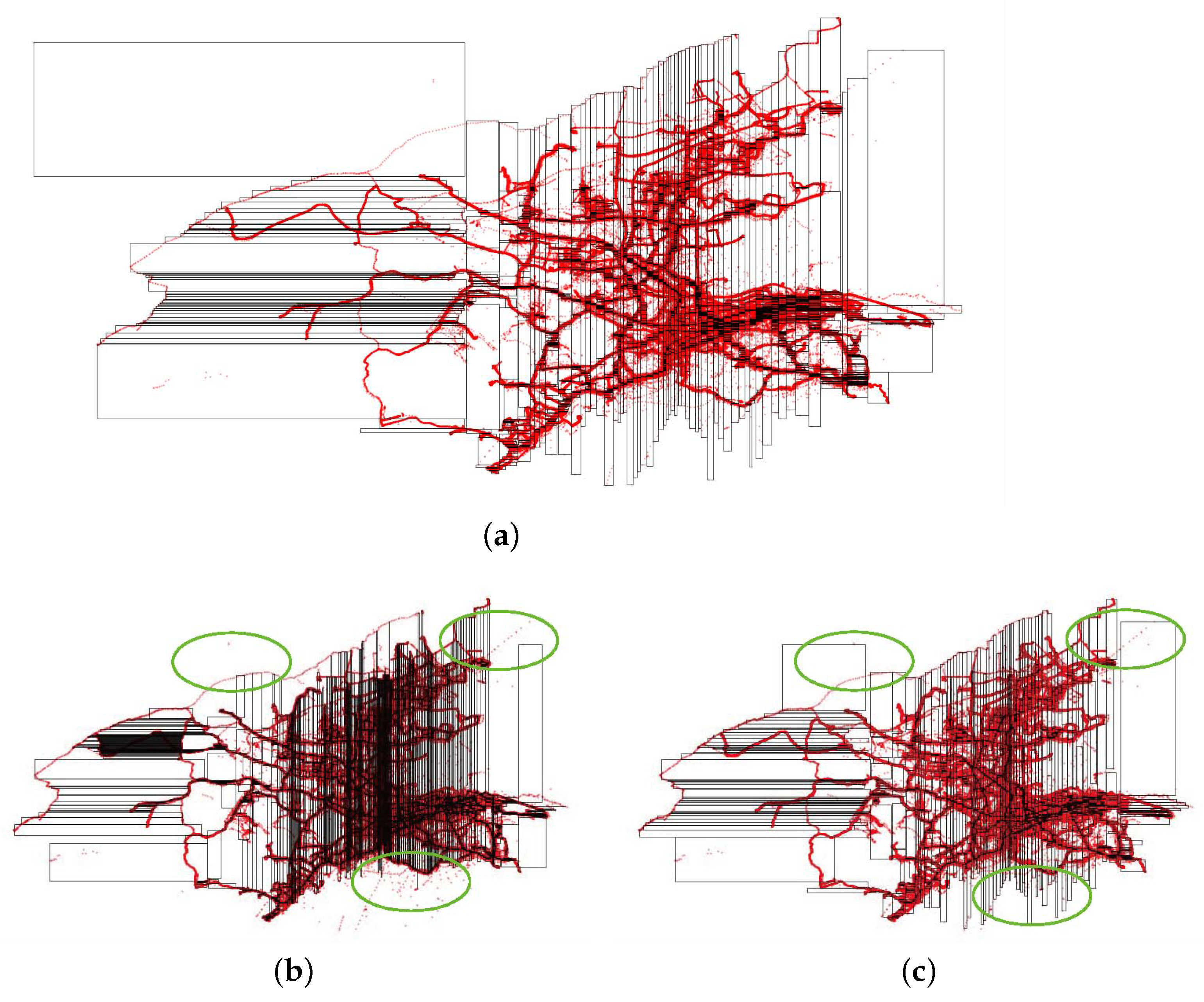
From the literature analysis, sampling-based methods are preferred because they are easy to implement and quickly obtain partitioning results, which facilitates the quick selection of suitable partitioning techniques. This is currently the most common choice for big data partitioning and is also integrated into most existing spatial data systems. However, due to the inherent instability of random sampling, as shown in Figure 1, the expression effect for sparse areas of skewed data is poor. It is obvious that random sampling does not capture elliptical region data, so there is a large gap between the calculation of partition boundaries and the actual partition. In this paper, we follow the sampling-based approach and propose a new histogram bucket sampling method for fast partitioning. The proposed histogram bucket sampling has three advantages over random sampling. First, its sampling set covers a wide range of partitions without generating new partition boundaries. Second, its sampling set cumulative distribution function and the original dataset cumulative distribution function error are bounded. Second, its sampling set cumulative distribution function and the original dataset cumulative distribution function error are bounded, this property can make the estimated spatial distribution of the sampling set approximately equal to the spatial distribution of the original dataset to a certain extent. Third, the partition boundaries obtained by its sampling set do not require excessive partition adjustment, reducing the fixed overhead of each map task in the MapReduce job. Histogram bucket sampling is a sampling method customized for the fast partitioning of spatial big data.
3. Symmetric Bin Sampling
In this section, we propose a new sampling method to compute partition boundaries. To quantify the quality of the results of the sampling-based solution in terms of the cumulative distribution function, we define the maximum error between a given approximate cumulative distribution function and the exact cumulative distribution function as follows.
Definition 1.
where represents the sampling rate. Since it is difficult to directly obtain the cumulative distribution function, the paper obtains this indirectly using the probability density function, such as Equations (2) and (3),
Maximum Error. We define the maximum error between the approximate cumulative distribution function and the exact cumulative distribution function as follows.
Given an error threshold , if holds, then holds, let , then holds.
When actually solving the probability density function, it is difficult to directly know the probability density function. To estimate the probability distribution, a histogram is constructed using a symmetric bin process that divides the variable values into discrete values. However, in practice, this value depends on the number of histogram bins, and the bin width for a given data range. Drawing on this idea, the two-dimensional space is divided into mutually disjointed bins. The bins are defined as follows:
Definition 2.
Histogram Bucket. Given a dataset , a histogram bucket is a subsets of :
For each in and , .
Approximately solve the two-dimensional probability density function using Equations (4) and (5)
where is the probability density function, is the frequency, is the number of datapoints in the bin , and is the total number of datasets. According to Equations (4) and (5), the two-dimensional probability density function of the sampling set is defined as Equations (6) and (7).
where is the probability density function of the sampling set, is the number of sampling points for the histogram bucket .
Lemma 1.
Assuming , if is true for , then for , constantly holds.
Proof.
□
Sampling the histogram bucket , the sampling rate is , and the sampling set is always established under the accurate calculation result. However, it is very time-consuming to accurately calculate the binned datapoints in a large dataset. Therefore, it is also very important to quickly estimate the value of within a certain error range in the research of histogram bucket sampling. In addition, you need to choose an appropriate bin size. Therefore, this paper mainly focuses on the above two aspects.
3.1. Selection of Bin Size
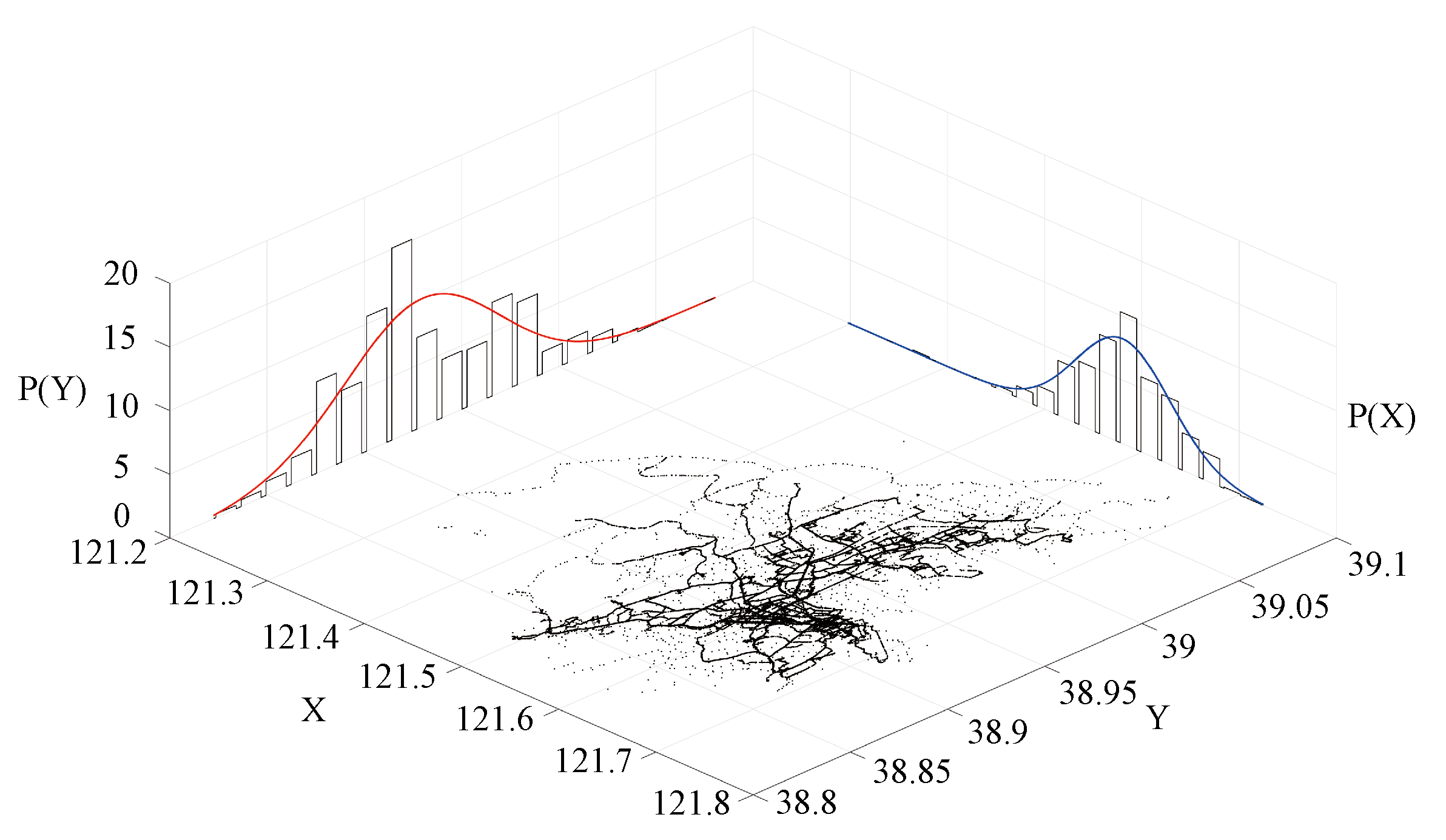
In our research environment, the amount of spatial data is huge, and the results of a parametric analysis of spatial distribution are not available. Therefore, we used a nonparametric modeling approach. In addition, as shown in Figure 2, the trajectory points in Figure 2 are typical spatial big data, and the black dots represent the trajectory points of the bus. It is observed that the trajectory points in low-longitude areas (such as Ganjingzi District) are sparse, most of the trajectory points are concentrated in the high-longitude part, and the spatial data present a skewed distribution. The widely adopted bucket width selection rule is to use Sturges’ rule [3] with bucket width .
where n is the total sample size, and represent the maximum and minimum values of the data range, respectively. The data are assumed to be normally distributed. However, when the data are not normally distributed, additional operations are required to address skewness. Scott’s rule [4] is based on the gradual theory, . This rule also assumes that the data are normally distributed. Freedman and Diaconis [18] extended Scott’s rule to give the bin width optimum for a non-normal distribution. For a set of empirical measurements sampled from some probability distribution, the Freedman–Diaconis rule is designed to minimize the integral of the squared difference between the histogram (that is, the relative frequency density) and the theoretical probability distribution density.
where is the 75th quantile value of the data, is the 25th quantile value of the data, and n is the number of samples, this paper uses the Freedman–Diaconis rule to calculate the bin length and width values of skewed data, such as Equations (8) and (9)
where and represent the 75th quantile and 25th quantile of .
3.2. Histogram Bucket Data Point Calculation
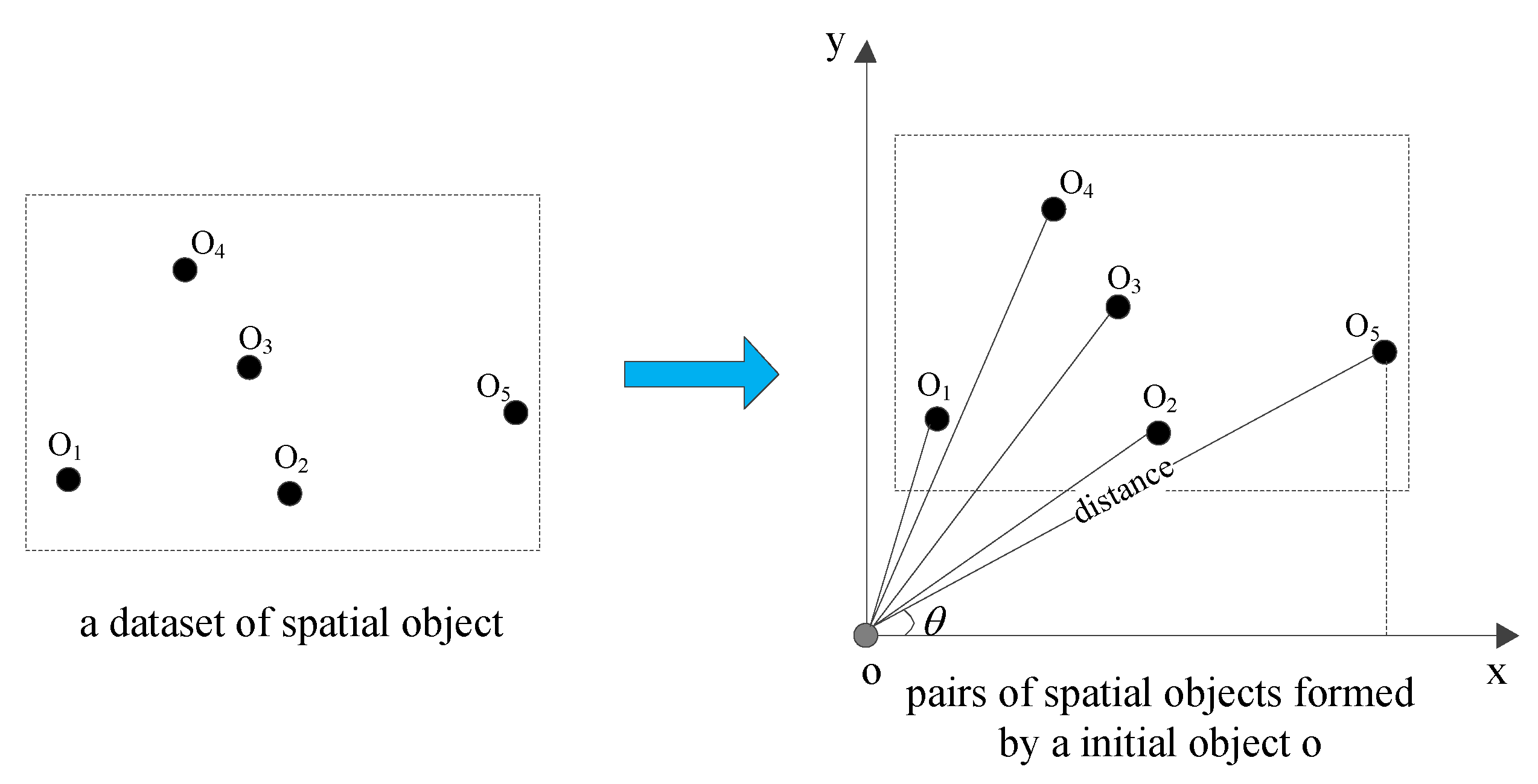
This section proposes a framework for fast computation of histogram bucket ; by establishing a functional relationship between the spatial offset and the number of spatial pairs, the approximate calculation of the value is realized within a certain error range. A description of space offset and space pair is given below.
Given a dataset , establish a spatial pair , , the spatial measure d, spatial offset refers to the smallest bounding rectangle (MBR) containing the spatial pair , MBR refers to the rectangle with the smallest perimeter L satisfying the relationship , which is uniquely represented by and d. MBR with a smaller distance is preferred. When d is equal, a smaller is selected when , and a larger is selected when . Figure 3 is an example of space pair and MBR, as shown in Equation (10).
Using the above concepts, define the spatial offset distribution histogram bucket, as follows:
Definition 3.
Spatially offset distribution bins (SODB). Let be a 2D dataset with datapoints, given a spatial pair , the spatial measure d, is defined as a two-dimensional array of buckets, Covering the field, there are square buckets, is expressed as: , , all bins have the same and values.
A simple way to calculate SODB see Algorithm 1. Initialize the square bucket first, then traverse the space pair to calculate the maximum value , , the minimum value , and , of on , , get the length and width of each square bucket, and store it in the square bucket array . Then, traverse the space pair to make it uniquely correspond to a square bucket, and finally return the function.
| Algorithm 1: SDOB() |
 |
The time complexity of Algorithm 1 includes:(1) Calculate all space-to-space offset values, namely, , where represents the complexity of each space offset calculation; (2) Sort all spatial offsets, that is, ; (3) Initialize the histogram bucket , namely ; (4) Traverse the space pair and calculate the value of each histogram bucket, that is, . In general, the time complexity of this method is . Obviously, when is large, the time complexity of this method is large, and cannot meet the needs of practical applications. Therefore, this paper designs the cumulative spatial offset distribution function to speed up the calculation of the spatial offset distribution histogram bucket, and the distribution function returns a jump function with respect to the spatial offset , as Definition 4.
Definition 4.
Cumulative Spatial Offset Distribution Function. Let be a 2D dataset with N datapoints, spatial pair , spatial measure d. For simplicity, we assume that the spatial domain is , , in the form of:
The functional relationship between and is Equation (11)
A simple way to calculate CSOD is shown in Algorithm 2. First initialize the MBR array, calculate the d value of all space pairs, and insert into the MBR array. Then, sort from small to large according to the smallest MBR perimeter, and calculate the cumulative spatial offset distribution function .
| Algorithm 2: CSOD() |
 |
The time complexity of Algorithm 2 is as follows: (1) Calculate all space-to-space offset values, that is, , where represents the complexity of each spatial offset calculation; (2) Sort all spatial offsets, that is, ; (3) Calculate the cumulative spatial offset distribution , that is, . In general, the time complexity of this method is . Obviously, this method is less practical when is large.
In the big data environment, it is difficult to calculate the value of quickly. Therefore, an approximate cumulative spatial offset distribution function with bounded error is designed in this paper to replace the value to speed up the sampling process, suppose the approximation is , as Definition 5.
Definition 5.
Approximate Cumulative Spatial Offset Distribution Function. Given a set of space pairs and a distance measure d and a fault tolerance threshold δ, Approximate cumulative spatial offset distribution returns a jump function with respect to spatial offset , :
For the calculation of , we use the Euclidean distance-based upper and lower boundary calculation method in the paper, as in Equations (12) and (13), keep unchanged, and the upper and lower boundaries of d are and .
We define the upper and lower boundary functions and .
Lemma 2.
If , then constant established.
Proof.
When exists, . Thence , the same can be proved . □
Lemma 3.
Knowing the upper and lower boundary functions, let . If and , constantly holds.
Proof.
Let , then , So only need , then is established. □
According to Equation (2) and Definition 4, we define the approximate spatial offset distribution histogram bucket as follows.
Definition 6.
Approximate Spatial Offset Distribution Histogram Buckets. Given a set of space pairs and a distance measure d and a fault tolerance threshold τ, a histogram bucket with length and width , approximate cumulative spatial offset distribution returns a function over bucket such that
For , is always true.
Lemma 4.
Given , suppose is the return result of the input dataset and the distance measure d, can be calculated by in time complexity .
Proof.
First prove that . According to Equation (6), the approximate spatial offset distribution histogram bucket is transformed into
□
The time complexity analysis: we derive from the computational complexity of . Computing requires i from 1 to and j from 1 to , a nested for loop is executed; therefore, the time complexity is .
3.3. Sampling
The histogram bucket is uniformly sampled according to the value of , and the sampling rate is , then = . Thence,
Therefore, the histogram bucket sampling according to the approximate spatial offset distribution not only satisfies Equation (1), but also improves the sampling efficiency.
4. Experiments
In this section, the experimental verification of the method of the paper will be carried out. The experimental setup is described in Section 4.1. In Section 4.2, a case study is conducted with a real bus trajectory dataset to demonstrate the applicability of ACSOD and ASODB. In Section 4.3, the accuracy of approximate solutions for ACSOD and ASODB is investigated, respectively. In Section 4.4, the values of the random sampling method and the method of this paper are compared on synthetic datasets and real datasets, respectively. Finally, in Section 4.5, synthetic and real datasets are used to evaluate the effectiveness of approximating partition boundaries.
4.1. Setting
Dataset Settings. The dataset consists of a synthetic dataset and a trajectory dataset. The size of the synthetic dataset is 3.67 GB and contains a total of 1,000,000 datapoints. The range [0,1] is skewed randomly. The trajectory dataset is 34.8 GB, contains 311,194,034 records.
Baseline methods. We evaluate the performance of the following two methods:
Random sampling: random sampling-based solutions randomly pick datapoints and compute an approximate cumulative distribution function with a fixed sampling rate .
Histogram Bucket Sampling: Error-bounded bin sampling is presented in Section 3.
Table 1 is the test value of sampling rate , error threshold and partition capacity size for scalability evaluation.
All methods are implemented in Python and Java. The performance of our method was measured using six common spatial partitioning techniques: Grid, Z-curve, H-curve, Kd-tree, STR [6], R*-Grove [13]. The single-threaded experiment (written in Python) runs on a PC with an Intel Core i7 4.20GHz processor and 32 GB of memory. The distributed experiments (written in Java) were run on a cluster of five machines with an Intel(R) Xeon(R) CPU E5-2620 2.40 GHz processor, 4 GB RAM, and runs Ubuntu 16.04.01 with Hadoop 2.7.7.
4.2. Accuracy Assessment
In this section, we will select a set of real trajectory datasets for experimental research to verify the applicability of ACSOD and ASODB under the bin sampling method, and demonstrate the advantages of the histogram bucket sampling method compared to the random sampling method that was previously used. In the process of processing these data, we will better show how to use histogram bucket sampling method to solve the limitations of using random sampling method for spatial big data partition processing; this results in better performance on data partition processing problems. To measure and compare the accuracy of two different sampling techniques in the experiments, we introduce a fault tolerance threshold indicator. When other data in the control experiments are the same, the fault tolerance thresholds of ACSOD and ASODB are compared using the two sampling methods. These were used to evaluate the applicability of ACSOD and ASODB and the accuracy of histogram bucket sampling.
We combine histogram bucket sampling techniques as well as random sampling techniques with existing spatial big data partitioning techniques for comparison. In the experiment, as Table 2 and Table 3, we used six different spatial big data partitioning techniques to divide the dataset into different datasets D, then chose spatial pairs in this dataset, , solving for distance measures and minimum bounding rectangles. The fault tolerance threshold of ACSOD and ASODB was caluclated using two different sampling methods to measure the accuracy of the two different sampling methods. The experiments in this section will verify the applicability of ACSOD and ASODB with two different sampling methods—histogram bucket sampling method and random sampling method—and calculate the fault tolerance threshold of the two using these two different sampling methods to verify their accuracy.
The above experimental data show the advantages of the histogram bucket sampling method in ACSOD and ASODB using different spatial big data partitioning techniques for data partitioning. In this experiment, we select spatial pairs and a fixed distance measure in the same dataset, and the generated minimum bounding rectangles are also identical. However, the traditional random sampling method cannot guarantee the worst-case overall distribution description when partitioning spatial data, resulting in excessive partition boundary adjustment operations, which reduces the fault tolerance rate of this method. Since the sampling set of the histogram bucket sampling technology covers a wide range of partitions, it is not necessary to generate new partition boundaries multiple times when processing large spatial data partitions. In addition, the partition boundaries obtained by the histogram bucket sampling technique do not require excessive partition adjustment, which reduces the fixed overhead of each map task in the MapReduce job to a certain extent. Thus, the fault tolerance threshold of the histogram bucket sampling technology is optimized, which makes the advantages of ACSOD and ASODB in the histogram bucket sampling technology more prominent. This verifies the accuracy of the histogram bucket sampling method.
4.3. Evalution
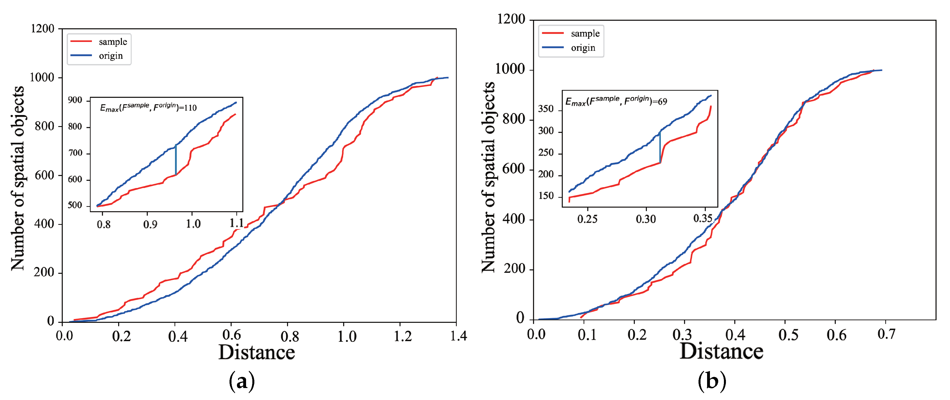
This section will quantify the approximation error of the bin sampling method proposed in this paper by using . Due to the huge amount of spatial data used in the experiment, the availability of the parametric analysis results of the spatial distribution is not high, and it is difficult to directly obtain the cumulative distribution function. Therefore, we indirectly obtained the E value using the probability density function. However, when actually solving the probability density function, it is difficult to directly know the probability density function. Usually, a histogram was used as a non-parametric density estimator to visualize the data and obtain various parameters and characteristics of the underlying density. Since in practice, this value depends on the number of histogram bins, and the bin width for a given data range. From this, we divided the two-dimensional space into mutually disjointed bins, then sampled the histogram bucket with a sampling rate of .
For intuitive expression, the two-dimensional cumulative distribution function was mapped on the XOZ surface. As shown in Figure 4, the sampling method in this paper is better than the random sampling method, because .
4.4. Evalution of Partition Boundary Effectiveness
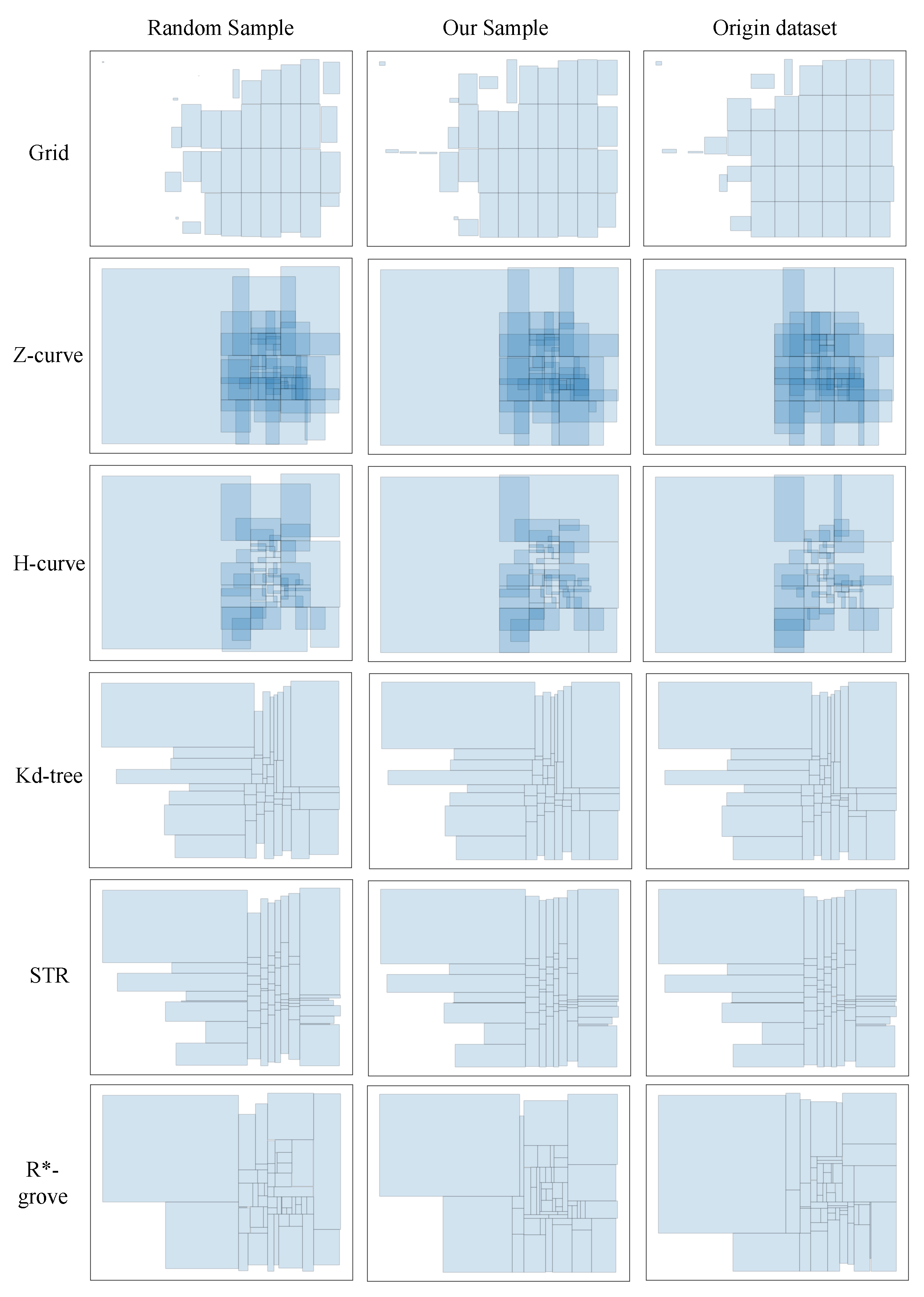
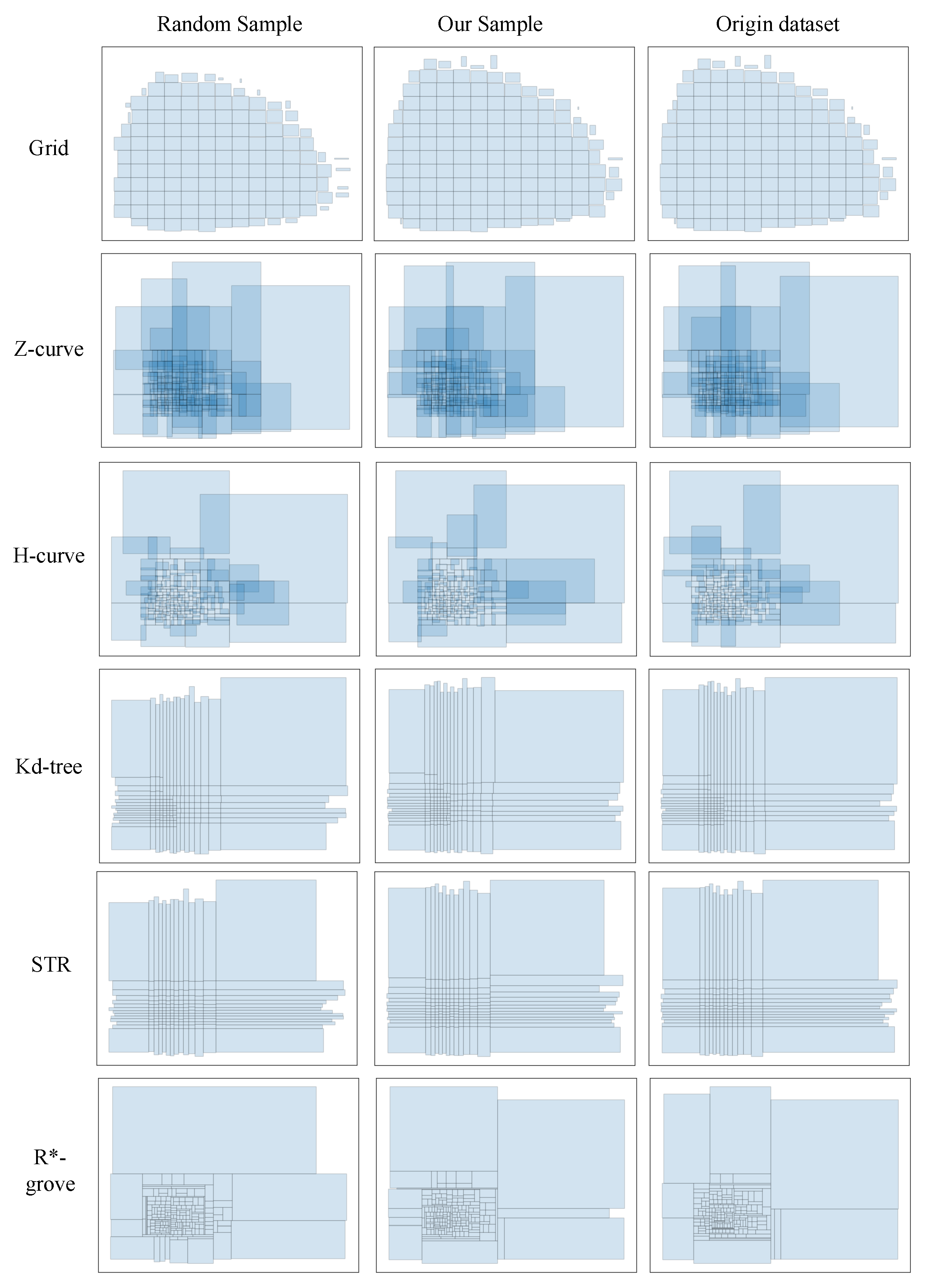
In this section, we will focus on the efficiency of our method using six partitioning techniques on different datasets. The performance of Grid, Z-curve, H-curve, Kd-tree, STR and R*-grove partitioning techniques is compared using a partition boundary coverage, as well as a comparison of the partition statistics. In each generated partition, the maximum capacity does not exceed the block size (set to 2 MB and 20 MB respectively). Therefore, the paper uses the partition load after data injection as a comparison indicator.
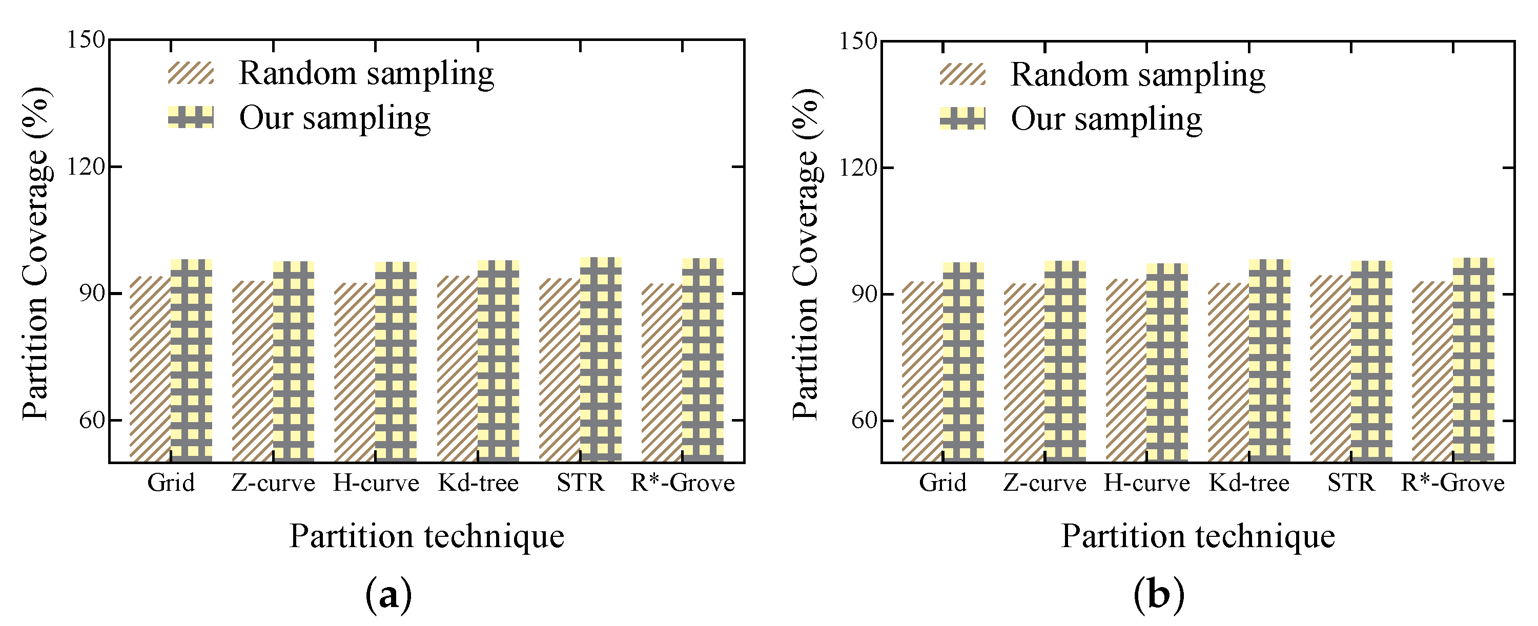
In the evaluation of the effectiveness of the partition boundary, the quantitative evaluation index is the partition coverage rate:
Statistics for each partition: total area of partitions, overlapping area of partitions, sum of partition boundaries, block utilization, standard deviation of partition size.
Total area of the zone:
where is the data block contained in each partition, , is the size of the i-th partition. represents the i-th partition, and is the area of the i-th partition.
Partition overlap area:
Total of partition boundaries:
where is the perimeter of the i-th partition.
Block utilization:
Partition size standard deviation:
where m is the number of partitions.
Figure 5 and Figure 6 show the advantages of the histogram bucket sampling method when using six common partitioning techniques for spatial big data partitioning on synthetic datasets and trajectory datasets, respectively. As shown in Figure 7, since the histogram bucket sampling method generates a wide range of data partitions when sampling the dataset. Thus, in each partition generated by the histogram bucket sampling method, the obtained partition coverage is much higher than that obtained using the random sampling method. Therefore, the histogram bucket sampling method is more efficient when processing large spatial data partitions.
4.5. Query Comparison
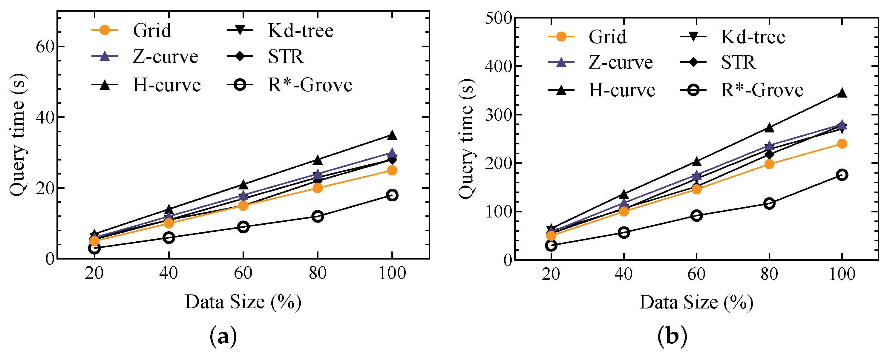
In this section, we will use a synthetic dataset and a trajectory dataset to verify the efficiency of histogram bucket sampling. We used Grid, Z-curve, H-curve, Kd-tree, STR, R*-Grove spatial partitioning techniques to verify the performance of the histogram bucket sampling method in range queries. Among them, Figure 8 show the response time of range queries using histogram bucket sampling on a synthetic dataset and a trajectory dataset, respectively. It can be seen that as the amount of query data increases, the query response time increases linearly. Combined with the relevant statistics in Table 4 and Table 5. The comparison found that in the initial stage, as the amount of data increased, the query response time linearly increased. When the amount of data increases to a certain amount, the response time of range queries using histogram bucket sampling method combined with Grid spatial data partitioning technology tends to be stable and no longer increases, and query efficiency can still be guaranteed.
5. Conclusions
In the MapReduce computing paradigm, partitioning a dataset into independent partitions is a key operation, as the degree of parallelism and overall performance directly depends on the initial partitioning technique. In this paper, we proposed a method of solving partition boundaries based on symmetric bin sampling, which computes an approximate cumulative distribution function within a certain margin of error to generate the best approximate partition boundaries for the analyzed dataset. This can be applied to the boundary solution of six commonly used partition methods. We applied it to synthetic and real datasets and compared the performance with random sampling techniques to highlight their differences and advantages. However, for skewed data, histogram bucket sampling is better than random sampling, but histogram bucket sampling is computationally complex. The future research directions includes how to design other sampling techniques to further improve performance, and a partition boundary solution that supported arbitrary data distribution. Another interesting direction is to present deep learning for partition boundary estimation.
Author Contributions
Conceptualization, R.T. and W.Z.; methodology, R.T. and T.C.; validation, R.T. and H.Z; investigation, R.T. and T.C.; data curation, T.C. and H.Z.; writing—original draft preparation, R.T. and T.C; writing—review and editing, H.Z. and F.W.; supervision, H.Z. and W.Z.; funding acquisition, H.Z., W.Z. and F.W. All authors have read and agreed to the published version of the manuscript.
Funding
This research was funded by the National Key Research and Development Program of China grant number 2020YFF0410947 and the National Natural Science Foundation of China grant number 62103072. Additional funding was provided by the China Postdoctoral Science Foundation grant number 2021M690502 and Shipping Joint Fund of Department of Science and Technology of Liaoning grant number 2020-HYLH-50.
Institutional Review Board Statement
Not applicable.
Informed Consent Statement
Not applicable.
Data Availability Statement
The dataset can be accessed upon request to the corresponding author.
Conflicts of Interest
The authors declare no conflict of interest.
References
- Li, R.Y.; Wang, R.B.; Huang, Y.C.; Liu, J.W.; Ruan, S.J.; He, T.F.; Bao, J.; Zheng, Y. JUST: JD Urban Spatio-Temporal Data Engine. In Proceedings of the 2020 IEEE 36th International Conference on Data Engineering (ICDE), Dallas, TX, USA, 20–24 April 2020; pp. 1558–1569. [Google Scholar] [CrossRef]
- Xie, D.; Li, F.; Yao, B.; Li, G.; Zhou, L.; Guo, M. Simba: Efficient In-Memory Spatial Analytics; SIGMOD: San Francisco, CA, USA, 2016; pp. 1071–1085. [Google Scholar] [CrossRef] [Green Version]
- Eldawy, A.; Alarabi, L.; Mokbel, M.F. Spatial partitioning techniques in Spatial-Hadoop. Proc. VLDB Endow. 2015, 8, 1602–1605. [Google Scholar] [CrossRef] [Green Version]
- Hughes, J.N.; Annex, A.; Eichelberger, C.N.; Fox, A.; Hulbert, A.; Ronquest, M. GeoMesa: A distributed architecture for spatio-temporal fusion. In Geospatial Informatics, Fusion, and Motion Video Analytics V; SPIE: Bellingham, WA, USA, 2015; p. 94730F. [Google Scholar] [CrossRef]
- Wu, X.; Ji, S. Comparative study on MapReduce and Spark for big data analytics. J. Softw. 2018, 29, 1770–1791. [Google Scholar]
- Alarabi, L.; Mokbel, M.F.; Musleh, M. ST-Hadoop: A MapReduce framework for spatio-temporal data. Geoinformatica 2018, 22, 785–813. [Google Scholar] [CrossRef]
- Vo, H.; Aji, A.; Wang, F. SATO: A Spatial Data Partitioning Framework for Scalable Query Processing. In Proceedings of the SIGSPATIAL, Dallas, TX, USA, 4–7 November 2014; pp. 545–548. [Google Scholar] [CrossRef]
- Cormode, G.; Duffield, N.G. Sampling for big data: A tutorial. In Proceedings of the 20th ACM SIGKDD International Conference on Knowledge Discovery and Data Mining, New York, NY, USA, 24–27 August 2014; p. 1975. [Google Scholar]
- Belussi, A.; Migliorini, S.; Eldawy, A. Skewness-Based Partitioning in Spatial Hadoop. ISPRS Int. J. Geo-Inf. 2020, 9, 201. [Google Scholar] [CrossRef] [Green Version]
- Hoeffding, W. Probability inequalities for sums of bounded random variables. J. Am. Stat. Assoc. 1963, 58, 13–30. [Google Scholar] [CrossRef]
- Serfling, R.J. Probability inequalities for the sum in sampling without replacement. Ann. Stat. 1973, 2, 39–48. [Google Scholar] [CrossRef]
- Vitter, J.S. Random sampling with a reservoir. ACM Trans. Math. Softw. 1985, 11, 37–57. [Google Scholar] [CrossRef] [Green Version]
- Kollios, G.; Gunopulos, D.; Koudas, N.; Berchtold, S. Efficient biased sampling for approximate clustering and outlier detection in large data sets. IEEE Trans. Knowl. Data Eng. 2003, 15, 1170–1187. [Google Scholar] [CrossRef]
- Yan, Y.; Chen, L.J.; Zhang, Z. Error-bounded sampling for analytics on big sparse data. Proc. VLDB Endow. 2014, 7, 1508–1519. [Google Scholar] [CrossRef] [Green Version]
- Li, Y.; Chow, C.Y.; Deng, K.; Yuan, M.; Zeng, J.; Zhang, J.D.; Yang, Q.; Zhang, Z.-L. Sampling Big Trajectory Data. In Proceedings of the 24th ACM International on Conference on Information and Knowledge Management (CIKM ’15), Melbourne, Australia, 18–23 October 2015; Association for Computing Machinery: New York, NY, USA, 2015; pp. 941–950. [Google Scholar] [CrossRef]
- Salloum, S.; Wu, Y.; Huang, J.Z. A Sampling-Based System for Approximate Big Data Analysis on Computing Clusters. In Proceedings of the 28th ACM International Conference on Information and Knowledge Management (CIKM ’19), Beijing, China, 3–7 November 2019; Association for Computing Machinery: New York, NY, USA, 2019; pp. 2481–2484. [Google Scholar] [CrossRef] [Green Version]
- Harsh, V.; Kale, L.; Solomonik, E. Histogram Sort with Sampling. In Proceedings of the 31st ACM Symposium on Parallelism in Algorithms and Architectures (SPAA ’19), Phoenix, AZ, USA, 22–24 June 2019; Association for Computing Machinery: New York, NY, USA, 2019; pp. 201–212. [Google Scholar] [CrossRef]
- Freedman, D.; Diaconis, P. On the histogram as a density estimator: L2 theory. Probab. Theory Relat. Fields 1988, 57, 453–476. [Google Scholar]
Figure 1.
Partition boundaries for whole data and sample data. This demonstrates that random sampling did not capture elliptical region points. (a) Whole data partition boundaries. (b) Random sampling partition boundaries. (c) Histogram bucket sampling partition boundaries.
Figure 1.
Partition boundaries for whole data and sample data. This demonstrates that random sampling did not capture elliptical region points. (a) Whole data partition boundaries. (b) Random sampling partition boundaries. (c) Histogram bucket sampling partition boundaries.

Figure 2.
An example of data distribution diagram.

Figure 3.
An example of spatial pair.

Figure 4.
Exact and approximate distribution of cumulative distribution function. (a) Random sampling. (b) Histogram bucket sampling.
Figure 4.
Exact and approximate distribution of cumulative distribution function. (a) Random sampling. (b) Histogram bucket sampling.

Figure 5.
Comparison of six partitioning techniques for trajectory data.

Figure 6.
Comparison of 6 partitioning techniques for synthetic data.

Figure 7.
Comparison of partition coverage. (a) Synthetic data. (b) Trajectory data.

Figure 8.
Query response time over two datasets. (a) Synthetic data. (b) Trajectory data.


Table 1.
Parameter settings.
| Parameter | Test Value |
|---|---|
| sampling rate | 2%, 4%, 6%, 8%, 10% |
| error threshold | 1%, 2%, 3%, 4%, 5% |
| size | 1 MB, 2 MB, 3 MB, 4 MB, 5 MB |
Table 2.
Random sampling.
| Spatial Pairs | Distance | Fault Tolerance Threshold | MBR | |
|---|---|---|---|---|
| ACSOD | 36.7 | 0.81 | (30, 36.7) | |
| ASODB | 34.6 | 0.86 | (30, 34.6) |
Table 3.
Histogram bucket sampling.
| Spatial Pairs | Distance | Fault Tolerance Threshold | MBR | |
|---|---|---|---|---|
| ACSOD | 36.7 | 0.97 | (30, 36.7) | |
| ASODB | 34.6 | 0.95 | (30, 34.6) |
Table 4.
Statistics for each partition of synthetic data.
| Grid | Z-Curve | H-Curve | KD-Tree | STR-Tree | R*-Grove | |
|---|---|---|---|---|---|---|
| P | 156/146/156 | 186/183/184 | 186/183/184 | 186/183/184 | 196/196/196 | 191/187/189 |
| TA | 74.94/65.0/74.95 | 114.37/107.63/102.17 | 87.1/67.54/69.69 | 74.48/68.42/77.85 | 43.4/36.6/43 | 142.17/121.79/123.9 |
| A | 242.58/199.68/242.58 | 176.39/184.95/131.32 | 51.13/42.52/38.35 | 32.37/29.92/34.13 | 1.68/0.96/1.45 | 182.73/147.38/127.01 |
| TPB | 304.72/275.73/304.74 | 231.64/211.86/210.53 | 175.04/162.92/157.25 | 275.46/254.53/275.69 | 188.52/168.21/186.23 | 195.89/176.24/188.14 |
| BUR | 58.43%/60.11%/57.61% | 69.59%/71.95%/72.41% | 70.12%/69.22%/72.69% | 72.58%/71.38%/71.56% | 91.08%/92.76%/91.59% | 82.58%/81.95%/82.52% |
| SD | 6.42/6.34/6.47 | 0.05/0.06/0.56 | 0.05/0.05/0.53 | 0.68/0.68/0.67 | 0.05/0.04/0.54 | 0.67/0.59/0.63 |
a Number of partitions. b Total area of partition. c Area of overlaping partitions. d Total partition boundary.
e Block utilization ratio. f Standard deviation of partition size. g The numbers represent the results of whole data,
histogram bucket sampling, and random sampling, respectively.
Table 5.
Statistics for each partition of trajectory data.
| Grid | Z-Curve | H-Curve | KD-Tree | STR-Tree | R*-Grove | |
|---|---|---|---|---|---|---|
| P | 38/40/41 | 50/50/53 | 50/50/53 | 50/50/53 | 64/64/64 | 51/51/54 |
| TA | 0.19/0.2/0.2 | 0.24/0.34/0.24 | 0.2/0.31/0.18 | 0.14/0.15/0.14 | 0.11/0.11/0.11 | 0.14/0.21/0.19 |
| A | 0.0/0.0/0.0 | 0.21/0.59.0.19 | 0.09/0.17/0.06 | 0.02/0.02/0.02 | 0.0/0.0/0.0 | 0.02/0.09/0.06 |
| TPB | 7.44/7.96/8.0 | 5.83/8.0/5.35 | 5.16/6.58/4.39 | 5.93/6.07/5.97 | 4.97/5.17/5.16 | 4.4/5.51/4.68 |
| BUR | 63.7%/62.47%/62.76% | 81.45%/64.91%/94.71% | 78.86%/67.54%/96.47% | 77.63%/78.09%/81.39% | 87.16%/80.61%/93.02% | 82.58%/81.95%/82.52% |
| SD | 4.95/4.87/49.87 | 0.02/0.02/0.16 | 0.02/0.02/0.17 | 0.7/0.7/6.56 | 0.01/0.02/0.17 | 0.05/0.06/0.52 |
Publisher’s Note: MDPI stays neutral with regard to jurisdictional claims in published maps and institutional affiliations. |
© 2022 by the authors. Licensee MDPI, Basel, Switzerland. This article is an open access article distributed under the terms and conditions of the Creative Commons Attribution (CC BY) license (https://creativecommons.org/licenses/by/4.0/).
Share and Cite
MDPI and ACS Style
Tian, R.; Chen, T.; Zhai, H.; Zhang, W.; Wang, F. A Method for Solving Approximate Partition Boundaries of Spatial Big Data Based on Histogram Bucket Sampling. Symmetry 2022, 14, 1055. https://0-doi-org.brum.beds.ac.uk/10.3390/sym14051055
AMA Style
Tian R, Chen T, Zhai H, Zhang W, Wang F. A Method for Solving Approximate Partition Boundaries of Spatial Big Data Based on Histogram Bucket Sampling. Symmetry. 2022; 14(5):1055. https://0-doi-org.brum.beds.ac.uk/10.3390/sym14051055
Chicago/Turabian StyleTian, Ruijie, Tiansheng Chen, Huawei Zhai, Weishi Zhang, and Fei Wang. 2022. "A Method for Solving Approximate Partition Boundaries of Spatial Big Data Based on Histogram Bucket Sampling" Symmetry 14, no. 5: 1055. https://0-doi-org.brum.beds.ac.uk/10.3390/sym14051055
Note that from the first issue of 2016, this journal uses article numbers instead of page numbers. See further details here.