
The Dual Expression of Parallel Equidistant Ruled Surfaces in Euclidean 3-Space


1
Department of Computer Technology, University of Gümüşhane, Gümüşhane 29000, Turkey
2
Department of Mathematics, University of Ordu, Ordu 52000, Turkey
3
Department of Economics, Management and Territory, University of Foggia, 71121 Foggia, Italy
*
Author to whom correspondence should be addressed.
Symmetry 2022, 14(5), 1062; https://0-doi-org.brum.beds.ac.uk/10.3390/sym14051062
Submission received: 27 April 2022
/
Revised: 16 May 2022
/
Accepted: 19 May 2022
/
Published: 22 May 2022
(This article belongs to the Special Issue Symmetry and Its Application in Differential Geometry and Topology)
Abstract
:In this study, we examine the dual expression of Valeontis’ concept of parallel p-equidistant ruled surfaces well known in Euclidean 3-space, according to the Study mapping. Furthermore, we show that the dual part of the dual angle on the unit dual sphere corresponds to the p-distance. We call these ruled surfaces we obtained “dual parallel equidistant ruled surfaces” and we briefly denote them with “DPERS”. Furthermore, we find the Blaschke vectors, the Blaschke invariants and the striction curves of these DPERS and we give the relationships between these elements. Moreover, we show the relationships between the Darboux screws, the instantaneous screw axes, the instantaneous dual Pfaff vectors and dual Steiner rotation vectors of these surfaces. Finally, we give an example, which we reinforce this article, and we explain all of these features with the figures on the example. Furthermore, we see that the corresponding dual curves on the dual unit sphere to these DPERS are such that one of them is symmetric with respect to the imaginary symmetry axis of the other.
1. Introduction
E. Study (1901) made the first applications to the geometry of dual numbers [1], which were first conceived by Clifford (1873) [2]. Dual numbers and dual vectors, which have been used by many researchers in various fields since then, have recently become important for studies in the space of lines. As for the concept of the ruled surfaces, they are determined with the movement of any line along any curve. The Study mapping is already based on the relationship between the geometry of the any line in and the geometry of any point on the unit dual sphere. That is, there exists one-to-one correspondence between the directed lines in line space and dual unit vectors on the dual vector space (-Modul). According to the correspondence principle, ruled surfaces specify a curve on the unit dual sphere, and this curve is called the dual spherical indicatrix of the ruled surface. The basic concepts related to the ruled surfaces in Euclidean space and on -Modul exist in many sources. Some of them are from Biran [3], Blaschke [4], Hacisalihoglu [5,6], Hagemann et al. [7], Muller [8], Ozdemir [9], Sabuncuoglu [10] and Senatalar [11]. Moreover, Ali and Abdel Aziz [12], Bilici [13] Oral and Kazaz [14], Saracoglu and Yayli [15,16] and Schaaf [17] have studied the various ruled surfaces. Moreover, several authors have worked on the integral invariants of closed ruled surfaces on the dual vector space [18,19,20,21]. As a new concept, Valeontis (1986) has defined parallel p-equidistant ruled surfaces (the tangent vectors of two ruled surfaces along the striction curves are parallel and at the same time the distance (p-distance) between the corresponding points of the polar planes of these surfaces is constant) and he has given their some features [22]. Based on this definition, Masal and Kuruoglu [23,24,25,26] have calculated some characteristic properties of these surfaces in Euclidean space and Minkowski space. Senyurt and As [27] have obtained some features of the parallel z-equidistant ruled surfaces obtained by paralleling normal vectors. Furthermore, Fenchel [28] has given the expression of the unit vector in direction of Darboux vector on the curve. In a similar vein, Sarioglugil et al. [29] and Senyurt [30] have studied on the ruled surface determined by the dual centroit curve. On the other hand, the dual vector space concept has been applied to research in kinematics, analysis and synthesis of spatial mechanisms, and many other fields. Some techniques obtained using dual vectors provide advantages in studies on robot kinematics [31]. Saglamer has [32] made robotic calculations in the kinematics of coordination between industrial robots using real and dual quaternion algebra. Sahiner [33] has studied differential properties of motion of a robot end-effector by using the curvature theory of dual spherical curves. In this paper, we comprehensively introduce the dual expression of parallel p-equidistant ruled surfaces in the space of lines according to the Study mapping. Furthermore, we show that the dual part of the dual angle on the unit dual sphere corresponds to the p-distance. Moreover, we give the relationships between the elements of these surfaces and finally reinforce these surfaces with an example. Finally, we see in this study that the corresponding dual curves on the dual unit sphere to these parallel equidistant ruled surfaces are such that one of them is symmetric with respect to the imaginary symmetry axis of the other. In the future, we are going to combine the result in the paper with singularity theory, sub-manifold theory, etc. from [34,35,36,37,38,39,40,41] to obtain new results and theorems. As a result of this study, further studies can be considered on the following research questions:
- What applications might this study have in the robot kinematics?
- What kind of contributions can this study make to the field of physics if it is studied in the different spaces?
2. Preliminaries
2.1. Some Preliminaries on -Modul
The addition and the multiplication operations on the dual numbers set
for the dual numbers A and B are stated as follows:
where a and are the real part and the imaginary part of the dual number A, respectively [2]. The set is a commutative ring with these operations. The division operation for the dual numbers A and B, with , is stated as the following:
The modulus of a dual number is just the absolute value of the real part .
The set , called the dual vector space, is a module with the following addition and scalar product operations on the ring and the set denoted by :
The inner and the vectorel product operations for are defined by, respectively:
The dual angle between the unit dual vectors and is stated as follows:
where is the real angle between and lines and is the shortest distance between and lines, while is unit dual vector [4,5]. For , the norm of the dual vector is defined by:
The set is called the unit dual sphere [5].
Theorem 1
(E. Study Mapping). The directed lines in are in one to one correspondence with the dual points of the unit dual sphere [1].
According to Study theorem, a ruled surface on the space of lines corresponds to a curve on the unit dual sphere. The dual equation of the ruled surface with the base curve and the generating line is defined by:
in the space of lines (). The dual spherical curve , with being a unit dual vector, represents by the ruled surface , where is the base curve of the ruled surface [4,5]. Let be the dual orthonormal moving system of the ruled surface , where . These unit dual vectors are defined by the following:
and are called Blaschke vectors [4]. There are the following relations between the Blaschke vectors and their derivative vectors:
and here:
are called Blaschke invariants [4]. The real and dual parts of these vectors are:
where is the Frenet frame, is the curvature and is the torsion of curve . According to Expression (7), the equations of the ruled surfaces are as follows:
If we derive the vectorial moment vectors according to s, we get:
The striction curve of the ruled surface is given as follows:
where the curvature and the torsion of this striction curve are and , respectively [4]. The Darboux screw are defined as follows [17]:
where is the Darboux vector of the curve and is the vectorial moment of the vector . The instantaneous screw axis of the ruled surface :
where is the instantaneous Pfaff vector of the curve and is the vectorial moment of the vector [4]. The dual Steiner rotation vector of the motion is found with the below equation:
where is the Steiner vector of the curve and is the vectorial moment of the vector [5]:
2.2. The Parallel p-Equidistant Ruled Surfaces in
Definition 1.
Let and be two ruled surfaces in If the following two conditions are satisfied, these ruled surfaces are called parallel p-equidistant ruled surfaces [22]:
- The generator vectors are parallel;
- The distance p between the polar planes at the suitable points of the ruled surfaces and is constant.
Let be Frenet frame at the point of the curve . If the generator vector of the ruled surface is taken the parametric expressions of these ruled surfaces are stated as follows:
3. The Dual Expression of Parallel Equidistant Ruled Surfaces in Euclidean 3-Space
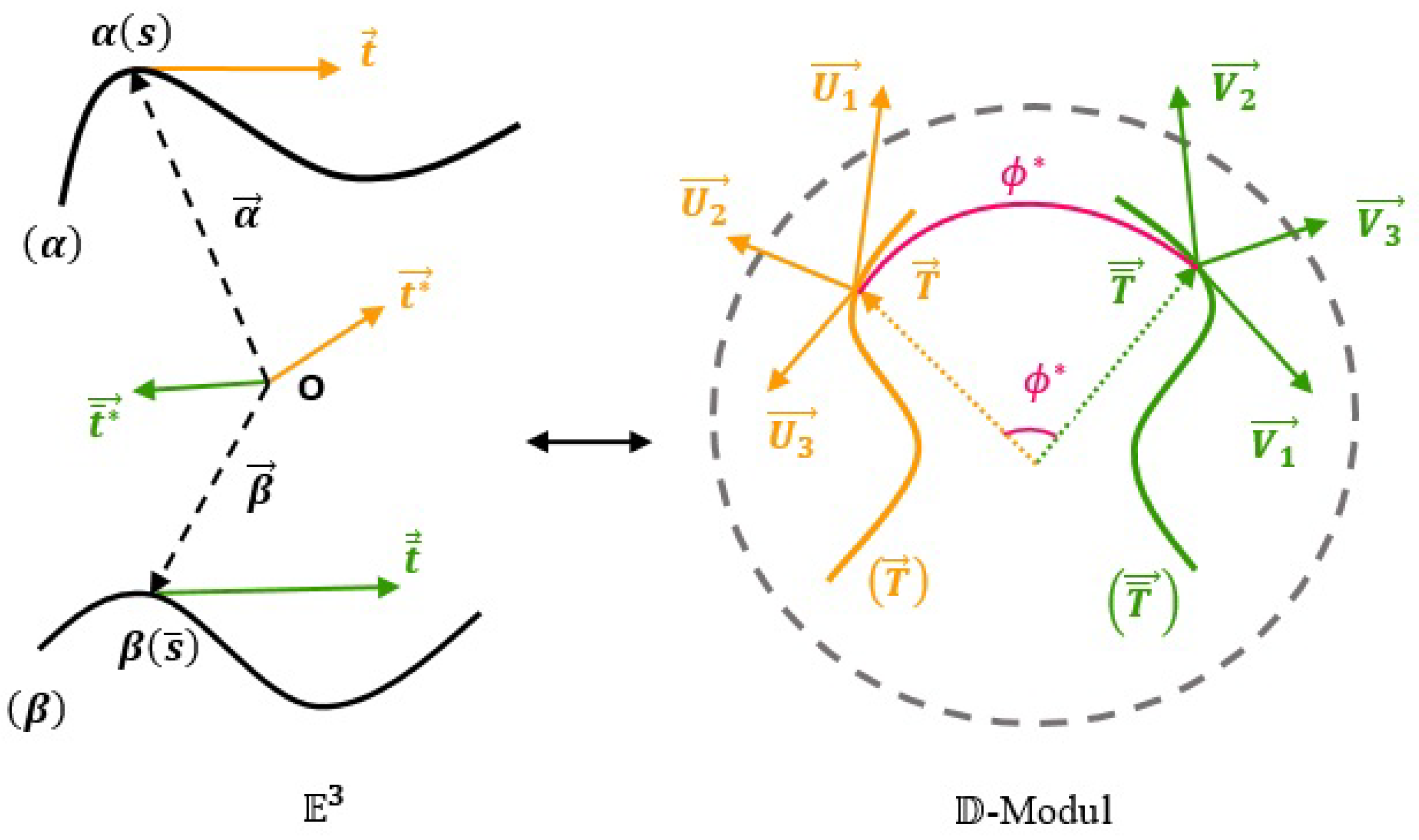
Let and be any two curves. Let and be the tangent vector and its vectorial moment of the curve and let and be the tangent vector and its vectorial moment of the curve , respectively. Furthermore, let be the dual angle between the dual vectors and on the unit dual sphere (or the dual arc length of the dual great circle passing through and dual points on the unit dual sphere, Figure 1), where the dual great circle of the dual unit sphere is the intersection of the sphere and a dual plane that passes through the center point of the dual sphere [5]. These dual vectors describe dual spherical curves on the dual unit sphere and the dual curves correspond to the ruled surfaces in .
From Expression (8), the Blaschke vectors of these ruled surfaces are given by the following (Figure 1):
where the axes and of these dual vectors intersect on the points of striction of these ruled surfaces and these points are on the axes and , respectively [4].
Definition 2 (Dual Parallel Equidistant Ruled Surfaces).
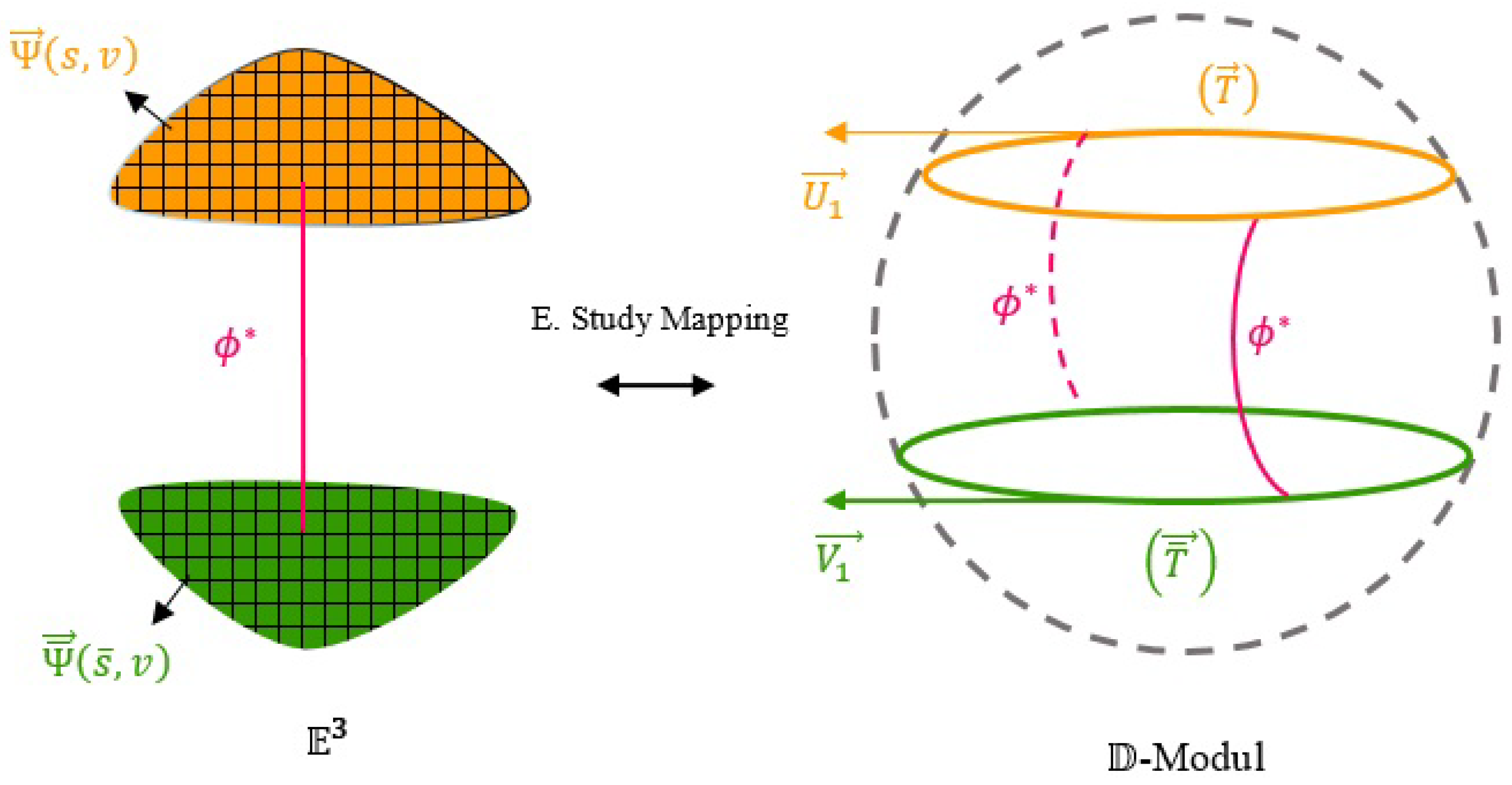
Let two curves be , and the unit tangent vectors be , and their vectorial moments be , of these curves in Euclidean 3-space , respectively. Furthermore, let the dual angle between the unit dual vectors and generated by these unit vectors (or the arc length between the corresponding dual points of the dual curves , described on the dual unit sphere of these unit dual vectors) be . If the angle (or the arc length) is non zero, constant and only dual , that is , the ruled surfaces corresponding to these curves according to Study mapping are called dual parallel equidistant ruled surfaces.
We will briefly denote these surfaces with DPERS from now on. The angle and length in question are explained in Figure 1 and Figure 2. Here, we draw imaginary figures on the unit dual sphere for these surfaces. According to this definition, the following results along the striction curves of these DPERS are obtained:
- The dual generator vectors and are parallel;
- The distance between these vectors at the corresponding points of the ruled surfaces is constant.
These results are equivalent to Valeontis’ expression in Definition 2. From Expression (7), the parametric expressions of the ruled surfaces corresponding in the space of lines to the dual curves and generated by the vectors and on -Modul are, respectively, written as follows:
where:
Furthermore, are the perpendicular projection distances on the unit vectors of the vector , respectively [22].
3.1. The Relationships between the Blaschke Vectors and the Blaschke Invariants and of DPERS
Theorem 2.
Let and be the Blaschke frames of DPERS and corresponding in the space of lines to the dual curves and on -Modul, respectively. There is the following relationship between the real and imaginary parts of these vectors:
Proof.
First, since the vectors and are parallel, . Here, and so and are parallel. We can take . Furthermore, since and , we get:
Second, from , we get and:
Finally, from , we get and:
□
Theorem 3.
Let , and , be the Blaschke invariants of DPERS and corresponding to the space of the lines to the dual curves and on -Modul, respectively. There are the following relationships between these invariants:
Proof.
If we derive the vector with respect to s, we get:
From the last equation, we have the following equations:
Likewise, if we derive the vector with respect to s, we get:
From the last equation, we have following equations:
□
Corollary 1.
The dual arc length between the corresponding dual points of DPERS and corresponding in the space of lines to the dual curves and on -Modul is found as follows:
This is the main conclusion of the article. This angle corresponds to the distance p in the dual expression of parallel p-equidistant surfaces; it is constant and nonzero.
If , from Expressions (21) and (27), the Blaschke frames and of DPERS and corresponding in the space of lines to the dual curves and on -Modul become equivalent.
In the corollaries obtained later in the paper (up to Section 3.3), we specifically chose as the generating line and thus considered the specific results in the Expressions (11) and (12).
Corollary 2.
For DPERS and corresponding in the space of lines to the dual curves and on -Modul, Expression (22) becomes as following:
Proof.
Corollary 3.
There is the following relationship between the arc-length parameters of the base curves of DPERS and corresponding in the space of lines to the dual curves and on -Modul:
Proof.
It is clear from Expression (26). □
In this corollary, if , from Expression (34), we get . That is, the arc-length parameters of the base curves of DPERS and corresponding in the space of lines to the dual curves and on -Modul are equivalent.
3.2. The Relationship between the Striction Curves of DPERS
Theorem 4.
Let and be the striction curves of DPERS and corresponding to the space of lines to the dual curves and on -Modul, respectively. There is the following relationship between these curves:
Proof.
From Expression (13), the striction curves’s equations of these ruled surfaces are obtained as follows:
If we use Expression (10), we obtain:
From Expression (21), we have:
If Expression (27) is used in the last expression, the proof is completed. □
Corollary 4.
The striction curves of DPERS and corresponding in the space of lines to the dual curves and on -Modul become their base curves.
Proof.
For these surfaces, if the vectors , , , are substituted in Expression (37), we get:
□
Corollary 5.
The Frenet frame, the curvature and the torsion of the striction curves of DPERS and corresponding in the space of lines to the dual curves and on -Modul are , , and , , , respectively.
3.3. The Relationships between the Darboux Screws and The Instantaneous Screw Axes of DPERS
In all theorems obtained in the following parts of the article, Expression (29) has been taken into account, as it will not change the general situation and for ease of operations.
Theorem 5.
Let and be the Darboux screws of DPERS and corresponding in the space of lines to the dual curves and on -Modul, respectively. There is the following relationship between these vectors:
Proof.
In this theorem, if , the Darboux screws of DPERS and corresponding in the space of lines to the dual curves and on -Modul are equivalent.
Theorem 6.
Let and be the instantaneous screws axes of DPERS and corresponding in the space of lines to the dual curves and on -Modul, respectively. There is the following relationship between these vectors:
Proof.
In this theorem, if , the instantaneous screw axes of DPERS and corresponding in the space of lines to the dual curves and on -Modul are equivalent.
Theorem 7.
Let be the dual angle between the vectors and , be the dual angle between the vectors and of DPERS and corresponding in the space of lines to the dual curves and on -Modul, respectively. There is the following relationship between these angles:
Proof.
From the solution of the equalities in Expression (50), we get:
Thus, from Expression (53), we arrive at the following relationship:
In this theorem, if , the dual angle between the vectors and , and the dual angle between the vectors and of DPERS and corresponding in the space of lines to the dual curves and on -Modul are equivalent.
Theorem 8.
Let be the dual angle between the vectors and , be the dual angle between the vectors and of DPERS and corresponding in the space of lines to the dual curves and on -Modul, respectively. There is the following relationship between the instantaneous screw axes and of these DPERS:
Proof.
Furthermore, the instantaneous screw axes in Expression (44) are obtained as:
Theorem 9.
Let and be the instantaneous dual Pfaff vectors of DPERS and corresponding in the space of lines to the dual curves and on -Modul, respectively. There is the following relationship between these vectors:
Proof.
From Expression (59), the instantaneous Pfaff vectors of the curves and are:
The vector moments and of these vectors are:
That is, the instantaneous Pfaff vectors of DPERS and corresponding in the space of lines to the dual curves and on -Modul are equivalent.
Furthermore, if (that is, the dual angle between the vectors and of ruled surface is only real), the vectors and in Expression (59) are equivalent to the vectors and in Expression (62). Thus, from the Expressions (58) and (63), and . That is, the Darboux screw axes and the instantaneous Pfaff vectors of DPERS and corresponding in the space of lines to the dual curves and on -Modul are equivalent, respectively.
Theorem 10.
Let and be the dual Steiner vectors of DPERS and corresponding in the space of lines to the dual curves and on -Modul, respectively. There is the following relationship between these vectors:
3.4. An Example For DPERS
Now, let us show all these results for the DPERS on an example to reinforce the study and make it easier for the reader to understand the subject. For this, first let us take two curves and in Euclidean 3-space. Furthermore, let us get the unit dual vectors and obtained with the tangent vectors , of these curves and the vector moments , of these vectors. Next, let us write the equations of the DPERS with base curves , and generating lines , . Furthermore, let us find Blaschke vectors, Blaschke invariants, Darboux screws and instantaneous Pfaff vectors of these ruled surfaces. Then, let us show the figures of these surfaces by drawing the surface equations we have obtained.
Example. Let us consider two helix curves:
Let us get , . In this case:
and the tangent vectors of these curves are obtained as follows:
Furthermore, the moment vectors of these vectors are computed, respectively, as follows:
and:
From Expression (19), the parametric expressions of the ruled surfaces corresponding in the space of lines to the dual curves and generated by the vectors and on -Modules are computed, respectively, as the following:
where we got . We find the Blaschke vectors and of DPERS and . The real and imaginary parts of these vectors are:
In Expression (20), if the inner product is applied to both sides of the equation:
with , and , respectively, we get:
From Expression (21), the relationships between real and imaginary parts of the Blaschke vectors and of DPERS and are obtained as follows:
Moreover, from Expression (28), the relations between the Blaschke invariants of these ruled surfaces are obtained as follows:
Furthermore, from Expression (37), the striction curves of these ruled surfaces are obtained as follows:
From the last expression, it is understood that the striction curves of these ruled surfaces are the base curves. That is, these ruled surfaces are drawn along the curves of striction. Furthermore, from Expression (40), the relationship between the Darboux screws is given as follows:
From Expression (42), the real and imaginary parts of these screws are:
In addition, from Expressions (50) and (53), the relationship between the dual angles between the vectors and and the vectors and is:
where:
Furthermore, from Expression (55), the relationship between the instantaneous screw axes of these surfaces is gotten as follows:
where, from Expression (59), the real and imaginary parts of these axes are:
Lastly, from Expression (60), the relationship between the instantaneous Pfaff vectors of these surfaces is found as follows:
where, from Expression (61) and (62), the real and imaginary parts of these vectors are:
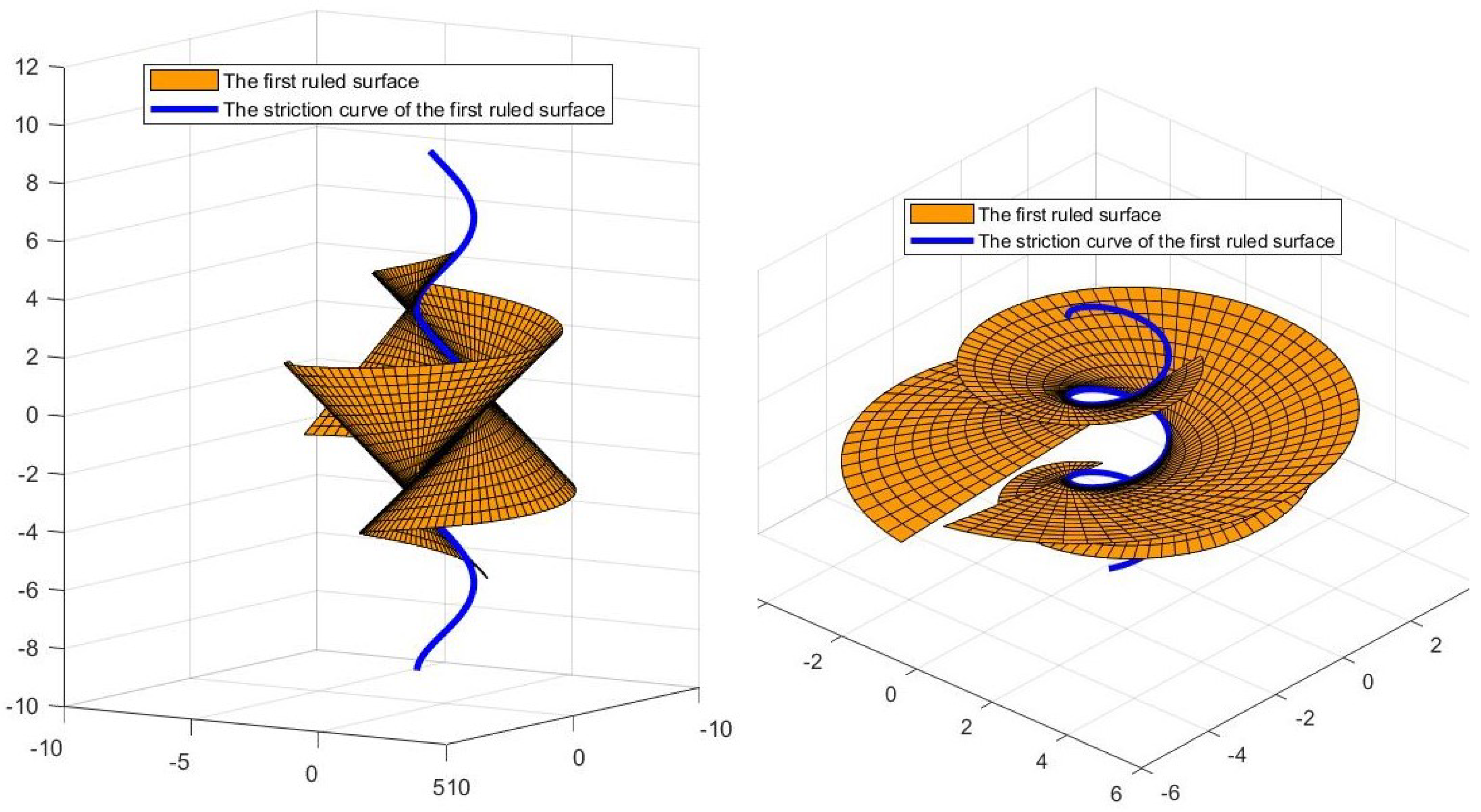
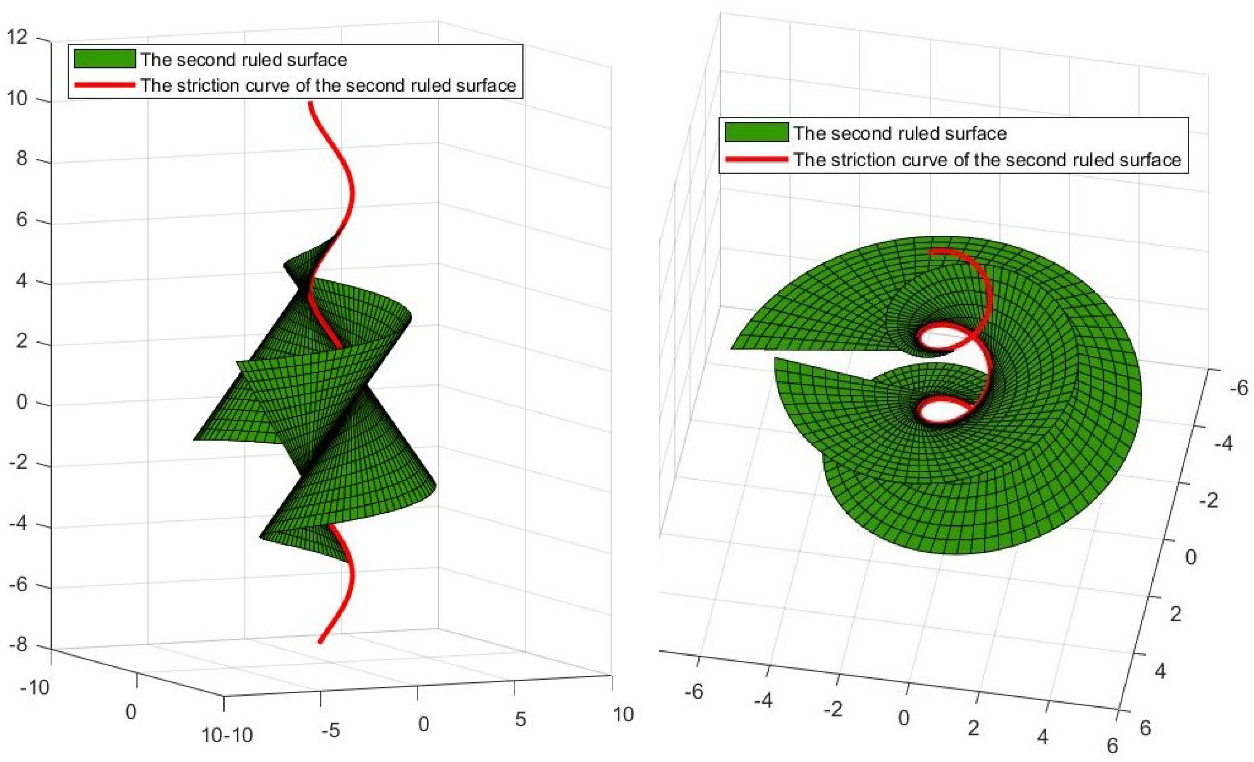
Let us now draw the figures of these ruled surfaces. If we get (the incremental values of in the range to ) and v = −5 : 1/2 : 5, we can draw the graphics in (Figure 3) for the ruled surface and we can draw the graphics in (Figure 4) for the ruled surface in
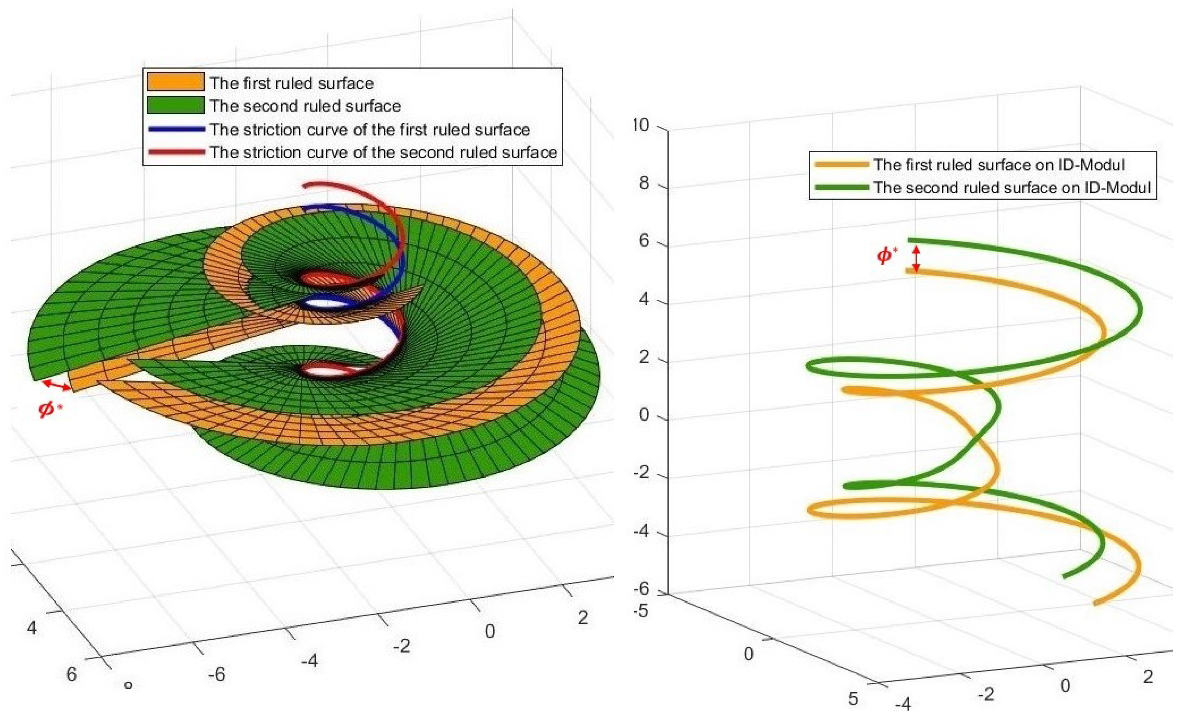
Now, let us draw these ruled surfaces together in , (on the left) in Figure 5. Furthermore, if we imagine that we show these DPERS on the dual unit sphere, they correspond to two dual parallel curves similar to that shown (on the right) in Figure 5. Here, and .
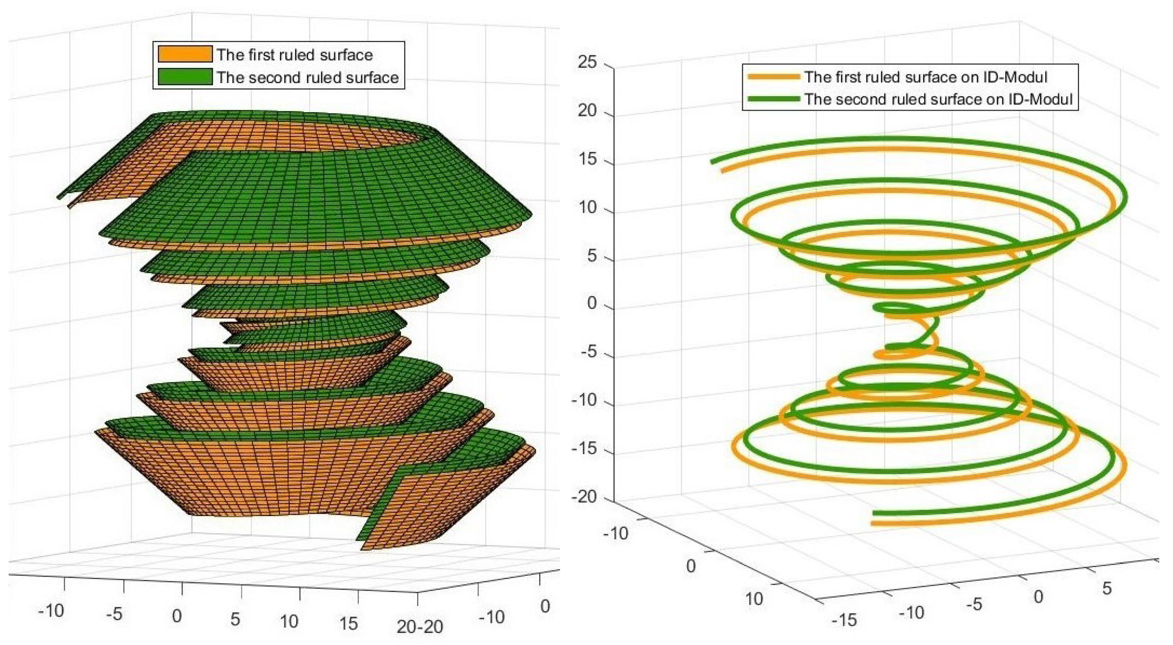
If we get and , we can draw the graphics in Figure 6 for the DPERS and in and on -Modul.
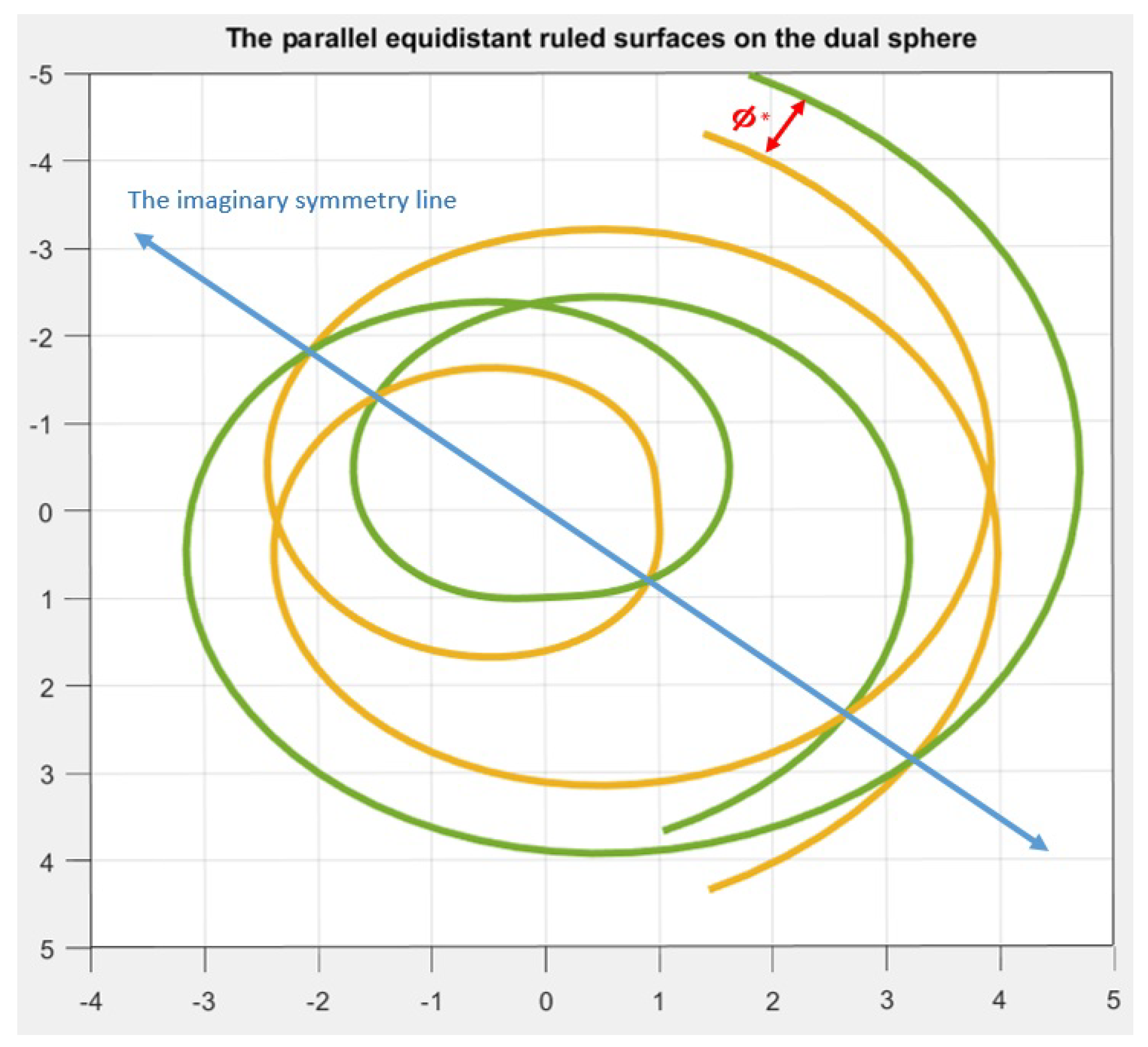
Finally, as seen in Figure 7, the dual curves corresponding to the DPERS on the dual unit sphere are such that one of them is symmetric with respect to the imaginary symmetry axis of the other.
4. Discussion and Conclusions
If the tangent vectors of two ruled surfaces along the striction curves are parallel and at the same time the distance (p-distance) between the corresponding points of the polar planes of these surfaces is constant, these surfaces are called parallel p-equidistant ruled surfaces. In this study, firstly, the dual expression of parallel p-equidistant ruled surfaces in the space of lines is given according to the Study mapping, and it is shown that the dual part of the dual angle on the unit dual sphere corresponds to the p-distance. Then, the relationships between Blaschke vectors, Blaschke invariants, the striction curves, the Darboux screws, the instantaneous screw axes, the instantaneous dual Pfaff vectors and the dual Steiner rotation vectors of these surfaces are expressed. Finally, an example for these surfaces is given and the drawings of these surfaces are made. The objective of this study is to make a new expansion for the parallel equidistant ruled surfaces on the dual vector space (-Modul). This expansion can also be studied by considering their principal normal vectors, binormal vectors or Darboux vectors instead of the tangent vectors of any two ruled surfaces, and thus, new parallel equidistant ruled surfaces can be obtained. Similarly, these surfaces can be studied in the Lorentzian space and the dual Lorentzian space, which have an important place in physics. In addition, these dual parallel equidistant ruled surfaces can be applied to studies on the robot kinematics.
Author Contributions
Conceptualization, S.G.M., S.Ş. and L.G.; methodology, S.G.M., S.Ş. and L.G.; validation, S.G.M., S.Ş. and L.G.; formal analysis, S.G.M., S.Ş. and L.G.; investigation, S.G.M.; resources, S.G.M., S.Ş. and L.G.; writing—original draft preparation, S.G.M.; writing—review and editing, S.G.M., S.Ş. and L.G.; visualization, S.G.M., S.Ş. and L.G.; supervision, S.Ş. and L.G. All authors have read and agreed to the published version of the manuscript.
Funding
This research received no external funding.
Institutional Review Board Statement
Not applicable.
Informed Consent Statement
Not applicable.
Data Availability Statement
Not applicable.
Acknowledgments
We, the authors, gratefully and most sincerely thank the reviewers who criticized and improved the quality of our article for their generous comments, corrections and contributions, as well as the editor of the journal who took care of our article.
Conflicts of Interest
The authors declare no conflict of interest.
Abbreviations
| DPERS | Dual Parallel Equidistant Ruled Surfaces |
References
- Study, E. Geometrie der Dynamen; Verlag Teubner: Leipzig, Germany, 1903. [Google Scholar]
- Clifford, W.K. Preliminary sketch of biquaternions. Proc. Lond. Math. Soc. 1873, 1, 381–395. [Google Scholar] [CrossRef]
- Biran, L. Differential Geometry Courses; AR-Publications: Istanbul, Turkey, 1981; pp. 81–88. [Google Scholar]
- Blaschke, W. Differential Geometry Courses; Istanbul University Publications: Istanbul, Turkey, 1949; pp. 332–345. [Google Scholar]
- Hacisalihoglu, H.H. The Motion Geometry and Quaternions Theory; Gazi University, Faculty of Science and Literature Publications: Ankara, Turkey, 1983; pp. 3–55. [Google Scholar]
- Hacisalioglu, H.H. Differential Geometry-II; Ankara University, Faculty of Science Publications: Ankara, Turkey, 1994; pp. 203–286. [Google Scholar]
- Hagemann, M.; Klawitter, D.; Lordick, D. Force Driven Ruled Surfaces. J. Geom. Graph. 2013, 17, 193–204. [Google Scholar]
- Muller, H.R. Kinematics Courses; Ankara University Press: Ankara, Turkey, 1963; pp. 240–251. [Google Scholar]
- Ozdemir, M. Quaternions and Geometry; Altin Nokta Press: İzmir, Turkey, 2020; pp. 150–182. [Google Scholar]
- Sabuncuoglu, A. Differential Geometry; Nobel Press: Ankara, Turkey, 2006. [Google Scholar]
- Senatalar, M. Differential Geometry (Curves and Surfaces Theory); Istanbul State Engineering and Architecture Academy Publications: Istanbul, Turkey, 1978; pp. 153–170. [Google Scholar]
- Ali, A.T.; Abdel Aziz, H.S.; Sorour, A.H. Ruled surfaces generated by some special curves in Euclidean 3-Space. J. Egypt. Math. Soc. 2013, 21, 285–294. [Google Scholar] [CrossRef] [Green Version]
- Bilici, M. On the Invariants of Ruled Surfaces Generated by the Dual Involute Frenet Trihedron. Commun. Fac. Sci. Univ. Ank. Ser. A1 Math. Stat. 2017, 66, 62–70. [Google Scholar]
- Oral, S.; Kazaz, M. Characterizations for Slant Ruled Surfaces in Dual Space. Iran. J. Sci. Technol. Trans. A Sci. 2017, 41, 191–197. [Google Scholar] [CrossRef]
- Saracoglu, S.; Yayli, Y. Ruled Surfaces and Dual Spherical Curves. Acta Univ. Apulensis 2012, 20, 337–354. [Google Scholar]
- Yayli, Y.; Saracoglu, S. Different Approaches to Ruled Surfaces. Univ. SüLeyman Demirel J. Sci. 2012, 7, 56–68. [Google Scholar]
- Schaaf, A.; Ravani, B. Geometric Continuity of Ruled Surfaces. Comput. Aided Geom. Des. 1998, 15, 289–310. [Google Scholar] [CrossRef]
- Bektas, Ö.; Senyurt, S. On Some Characterizations of Ruled Surface of a Closed Timelike Curve in Dual Lorentzian Space. Adv. Appl. Clifford Algebr. 2012, 22, 939–953. [Google Scholar] [CrossRef] [Green Version]
- Gursoy, O. The dual angle of the closed ruled surfaces. Mech. Mach. Theory 1990, 25, 131–140. [Google Scholar] [CrossRef]
- Hacisalihoglu, H.H. Acceleration Axes in Spatian Kinematics I. Commun. Fac. Sci. Univ. Ank. Ser. Math. Stat. 1971, 20, 1–15. [Google Scholar]
- Hacisalihoglu, H.H. On the pitch of a closed ruled surfaces. Mech. Mach. Theory 1972, 7, 291–305. [Google Scholar] [CrossRef]
- Valeontis, I. Parallel P-Äquidistante Regelflachen Manuscripta. Mathematics 1986, 54, 391–404. [Google Scholar]
- Masal, M.; Kuruoglu, N. Some Characteristic Properties of the Parallel P-Equidistant Ruled Surfaces in The Euclidean Space. Pure Appl. Math. Sci. 1999, 50, 35–42. [Google Scholar]
- Masal, M.; Kuruoglu, N. Some Characteristic Properties of the Shape Operators of Parallel p-Equidistant Ruled Surfaces. Bull. Pure Appl. Sci. 2000, 19, 361–364. [Google Scholar]
- Masal, M.; Kuruoglu, N. Spacelike parallel pi-equidistant ruled surfaces in the Minkowski 3-space R13. Algebr. Groups Geom. 2005, 22, 13–24. [Google Scholar]
- Senyurt, S.; Gur Mazlum, S.; Grilli, G. Gaussian curvatures of parallel ruled surfaces. Appl. Math. Sci. 2020, 14, 171–183. [Google Scholar] [CrossRef]
- As, E.; Senyurt, S. Some Characteristic Properties of Parallel z-Equidistant Ruled Surfaces. Hindawi Publ. Corp. Math. Probl. Eng. 2013, 2013, 587289. [Google Scholar]
- Fenchel, W. On the Differential Geometry of Closed Space Curves. Bull. Am. Math. Soc. 1951, 57, 44–54. [Google Scholar] [CrossRef] [Green Version]
- Sarioglugil, A.; Senyurt, S.; Kuruoglu, N. On the Integral Invariants of the Closed Ruled Surfaces Generated by a Parallel p-Equidistant Dual Centroit Curve in the Line Space. Hadron. J. 2011, 34, 34–47. [Google Scholar]
- Senyurt, S. Integral Invariants of Parallel P-Equidistant Ruled Surfaces Which Are Generated by Instantaneous Pfaff Vector. Ordu Univ. Sci. Tech. J. 2012, 2, 13–22. [Google Scholar]
- Chittawadigi, R.G.; Hayat, A.A.; Saha, S.K. Geometric model identification of a serial robot. In Proceedings of the International Symposium on Robotics and Mechatronics, Singapore, 2–5 October 2013. [Google Scholar]
- Saglamer, E. Kinematically Modelling and Solution of Motion Coordination of Multi Robots with Quaternions. Master’s Thesis, Istanbul Technical University Institute of Sciences, Istanbul, Turkey, 2008. [Google Scholar]
- Sahiner, B.; Kazaz, M.; Ugurlu, H.H. A Dual Method to Study Motion of a Robot End-Effector. J. Inform. Math. Sci. 2018, 10, 247–259. [Google Scholar] [CrossRef]
- Li, Y.L.; Dey, S.; Pahan, S.; Ali, A. Geometry of conformal η-Ricci solitons and conformal η-Ricci almost solitons on Paracontact geometry. Open Math. 2022, 20, 1–20. [Google Scholar] [CrossRef]
- Li, Y.L.; Zhu, Y.S.; Sun, Q.Y. Singularities and dualities of pedal curves in pseudo-hyperbolic and de Sitter space. Int. J. Geom. Methods Mod. Phys. 2021, 18, 1–31. [Google Scholar] [CrossRef]
- Li, Y.L.; Lone, M.A.; Wani, U.A. Biharmonic submanifolds of Kähler product manifolds. AIMS Math. 2021, 6, 9309–9321. [Google Scholar] [CrossRef]
- Li, Y.L.; Alkhaldi, A.H.; Ali, A.; Laurian-Ioan, P. On the Topology of Warped Product Pointwise Semi-Slant Submanifolds with Positive Curvature. Mathematics 2021, 9, 3156. [Google Scholar] [CrossRef]
- Li, Y.L.; Ali, A.; Mofarreh, F.; Alluhaibi, N. Homology groups in warped product submanifolds in hyperbolic spaces. J. Math. 2021, 2021, 8554738. [Google Scholar] [CrossRef]
- Li, Y.L.; Ali, A.; Ali, R. A general inequality for CR-warped products in generalized Sasakian space form and its applications. Adv. Math. Phys. 2021, 2021, 5777554. [Google Scholar] [CrossRef]
- Li, Y.L.; Ali, A.; Mofarreh, F.; Abolarinwa, A.; Ali, R. Some eigenvalues estimate for the ϕ-Laplace operator on slant submanifolds of Sasakian space forms. J. Funct. Space 2021, 2021, 6195939. [Google Scholar]
- Li, Y.L.; Abolarinwa, A.; Azami, S.; Ali, A. Yamabe constant evolution and monotonicity along the conformal Ricci flow. AIMS Math. 2022, 7, 12077–12090. [Google Scholar] [CrossRef]
Figure 1.
The dual spherical curves and their Blaschke vectors (the imaginary figure for -Modul).

Figure 2.
The dual parallel equidistant ruled surfaces.

Figure 3.
The first ruled surface and its striction curve in .

Figure 4.
The second ruled surface and its striction curve in .

Figure 5.
The dual parallel equidistant ruled surfaces for .

Figure 6.
The dual parallel equidistant ruled surfaces for .

Figure 7.
The dual parallel equidistant ruled surfaces on dual unit sphere.

Publisher’s Note: MDPI stays neutral with regard to jurisdictional claims in published maps and institutional affiliations. |
© 2022 by the authors. Licensee MDPI, Basel, Switzerland. This article is an open access article distributed under the terms and conditions of the Creative Commons Attribution (CC BY) license (https://creativecommons.org/licenses/by/4.0/).
Share and Cite
MDPI and ACS Style
Gür Mazlum, S.; Şenyurt, S.; Grilli, L. The Dual Expression of Parallel Equidistant Ruled Surfaces in Euclidean 3-Space. Symmetry 2022, 14, 1062. https://0-doi-org.brum.beds.ac.uk/10.3390/sym14051062
AMA Style
Gür Mazlum S, Şenyurt S, Grilli L. The Dual Expression of Parallel Equidistant Ruled Surfaces in Euclidean 3-Space. Symmetry. 2022; 14(5):1062. i.org/10.3390/sym14051062
Chicago/Turabian StyleGür Mazlum, Sümeyye, Süleyman Şenyurt, and Luca Grilli. 2022. "The Dual Expression of Parallel Equidistant Ruled Surfaces in Euclidean 3-Space" Symmetry 14, no. 5: 1062. https://0-doi-org.brum.beds.ac.uk/10.3390/sym14051062
Note that from the first issue of 2016, this journal uses article numbers instead of page numbers. See further details here.