Hesitant Fuzzy Variable and Distribution

Abstract

In recent decades, the hesitant fuzzy set theory has been used as a main tool to describe the hesitant fuzzy phenomenon, which usually exists in multiple attributes of decision making. However, in the general case concerning numerous decision-making problems, values of attributes are real numbers, and some decision makers are hesitant about these values. Consequently, the possibility of taking a number contains several possible values in the real number interval [0, 1]. As a result, the hesitant possibility of hesitant fuzzy events cannot be inferred from the given hesitant fuzzy set which only presents the hesitant membership degree with respect to an element belonging to this one. To address this problem, this paper explores the axiomatic system of the hesitant possibility measure from which the hesitant fuzzy theory is constructed. Firstly, a hesitant possibility measure from the pattern space to the power set of [0, 1] is defined, and some properties of this measure are discussed. Secondly, a hesitant fuzzy variable, which is a symmetric set-valued function on the hesitant possibility measure space, is proposed, and the distribution of this variable and one of its functions are studied. Finally, two examples are shown in order to explain the practical applications of the hesitant fuzzy variable in the hesitant fuzzy graph model and decision-making considering hesitant fuzzy attributes. The relevant research results of this paper provide an important mathematical tool for hesitant fuzzy information processing from another new angle different from the theory of hesitant fuzzy sets, and can be utilized to solve decision problems in light of the hesitant fuzzy value of multiple attributes.

1. Introduction

The hesitant fuzzy set, which is an extended version of the fuzzy set [1], is characterized by hesitant membership grades that contain several possible real numbers in an interval [0, 1] [2], and is illustrated by decomposition theorems and extension principles concerning this concept [3]. In the 2010s, the theory and application in respect to the hesitant fuzzy set were investigated for making a group decision. For one thing, Xia et al. introduced some operators with respect to hesitant fuzzy sets and utilized these operators to deal with hesitant fuzzy information [4]. For another thing, on the basis of the assumption that elements of a hesitant fuzzy set are increasingly arranged and the length of two elements is the same, Xia et al. proposed some distance measures of hesitant fuzzy sets [5]. Consequently, they considered connections of these measures and presented several kinds of similarity measures for hesitant fuzzy sets [6]. After that, Xia et al. extended the preference relation to the hesitant fuzzy case and introduced some relevant properties [7]. Zhang et al. developed the normalization extension and group extension concerning the hesitant fuzzy preference relation for describing the consensus process in terms of hesitant fuzzy information [8,9]. Zhu et al. defined a consensus index for measuring the agreement between the group and arbitrary individual hesitant fuzzy preference relation considering hesitant fuzzy attributes [10]. Xu et al. introduced a consensus model with respect to the hesitant fuzzy preference relation and presented feedback mechanisms [11]. Zhang et al. established some consistency models in order to obtain missing elements for incomplete hesitant fuzzy preference relations. In addition, some aggregation operators have been introduced to fuse hesitant fuzzy sets in decision making [12,13,14,15,16]. These operators are able to provide powerful guarantees for decision makers to handle complex situations. In order to determine better group decisions, some methods based on hesitant fuzzy sets or the extended hesitant fuzzy sets have been introduced, for instance, the hesitant fuzzy TOPSIS [17], m-polar hesitant fuzzy TOPSIS approach [18], hesitant fuzzy PROMETHEE [19], hesitant fuzzy ELECTRE [20], hesitant fuzzy VIKOR [21], hesitant fuzzy TODIM [22], hesitant fuzzy QUALIFLEX [23], hesitant N-soft sets decision method [24], necessary and possible hesitant fuzzy sets method [25], dual extended hesitant fuzzy sets method [26], hesitant fuzzy N-soft sets method [27] and hesitant fuzzy LINMAP [28].

In recent years, the hesitant fuzzy set theory has been used as a main mathematical tool to describe the hesitant fuzzy phenomenon in the research of multiple attributes of decision making. However, a hesitant fuzzy set only presents several possible values on the unit interval [0, 1], which defines the hesitant membership of an element belonging to this hesitant fuzzy set, and the hesitant possibility of hesitant fuzzy events cannot be inferred from the given hesitant fuzzy sets [2]. Because it is the general case that the value of an attribute is a real number in multiple attributes of group decision making problems, decision makers are hesitant about this real number corresponding to the attribute, that is, the possibility of taking this real number contains several possible values in the interval [0, 1]. In this situation, the hesitant fuzzy model is more appropriate to describe hesitant fuzzy events. On the one hand, probability measures can explain the probability of the occurrence of random events and a random variable is essentially a measurable function from the probability measure space to the real value line [29]. On the other hand, as a pair of dual measures, the possibility measure and necessity measure can show the possibility and necessity of fuzzy events, and the basic concept of fuzzy theory is a fuzzy variable, which is a measurable function from measure space to the real set. Similarly, a credibility measure is the self-dual fuzzy measure, which can measure the credibility of fuzzy events [30,31,32]. Therefore, the axiomatic system with respect to the hesitant possibility of hesitant fuzzy events has important theoretical significance in the study of the hesitant fuzzy phenomenon; this axiomatic framework is based on the hesitant fuzzy variable, which is a symmetric set-valued function with respect to the union operation of the hesitant fuzzy variable, and can provide theoretical support for hesitant fuzzy information processing.

In this paper, the main contributions include several points: (1) Proposing a hesitant possibility measure, a hesitant necessary measure and a hesitant credibility measure and studying some properties with respect to these three set-valued measures. (2) Defining a hesitant fuzzy variable on the hesitant possibility measure space, and discussing the distribution of this variable and one of its functions and listing several common hesitant fuzzy variables, including triangle, trapezoid, normal and exponential types. (3) Introducing the concept of the hesitant fuzzy graph based on the proposed hesitant fuzzy variable. The rest of this paper is structured as follows: In Section 2, preliminaries are illustrated. Section 3 presents the axiomatic system with respect to the hesitant possibility of hesitant fuzzy events. Two applications are showed in Section 4. Some conclusions and future works are stated in the final section.

2. Preliminaries

Definition 1

[33]. If $\Gamma$ is a domain of discourse and $I$ is any index set, an ample field $\mathcal{A}$ is a collection of subsets of $\Gamma$ with the following conditions:

(1)

$\Gamma \in \mathcal{A}$;

(2)

$A\in \mathcal{A}\Rightarrow \Gamma \backslash A\in \mathcal{A}$;

(3)

$B_k\in \mathcal{A}$,$k\in I$$\Rightarrow {\displaystyle \underset{k\in I}{\cup }{B}_k}\in \mathcal{A}$.

$\left(\Gamma ,\mathcal{A}\right)$ is called an ample space. Evidently,$\left(\Gamma ,\mathcal{P}(\Gamma )\right)$ is a special amplespacein which$\mathcal{P}(\Gamma )$ is the power set of $\Gamma$.

Definition 2

[34]. Let $\left(\Gamma ,\mathcal{A}\right)$ be an ample space. A fuzzy measure on an ample field $\mathcal{A}$ is defined by a function $\mu$ from $\mathcal{A}$ to $[0,\infty ]$ with two conditions:

(1)

$\mu (\varphi )=0$;

(2)

$B_1\in \mathcal{A}$, $B_2\in \mathcal{A}$, $B_1\subset B_2$$\Rightarrow \mu (B_1)\le \mu (B_2)$.

Particularly, $\mu :\mathcal{A}\to [0,\infty ]$ is called the lower semicontinuous when:

$$B_n\in \mathcal{A},n=1,2,\cdots ,B_1\subset B_2\subset \cdots \Rightarrow \underset{n\to \infty }{\lim }\mu (B_n)=\mu ({\displaystyle {\cup }_{n=1}^{\infty }{B}_n}).$$

$\mu :\mathcal{A}\to [0,\infty ]$ is called upper semicontinuous when:

$$B_n\in \mathcal{A},n=1,2,\cdots ,B_1\supset B_2\supset \cdots \Rightarrow \underset{n\to \infty }{\lim }\mu (B_n)=\mu ({\displaystyle {\cap }_{n=1}^{\infty }{B}_n}).$$

Definition 3

[35]. Let $\left(\Gamma ,\mathcal{A}\right)$ be an ample space $\Gamma$ and $I$ be an arbitrary index set. A set function $Pos:$$\mathcal{A}\to [0,1]$ is called the possibility measure on $\mathcal{A}$ when the following conditions hold:

(1)

$Pos(\varphi )=0,Pos(\Gamma )=1$;

(2)

$B_k\in \mathcal{A}$, $k\in I$$\Rightarrow Pos\left({\displaystyle {\cup }_{k\in I}{B}_k}\right)=\underset{k\in I}{\sup }Pos\left(B_k\right)$.

The triple ($\Gamma$, $\mathcal{A}$, $Pos$) is defined as a possibility measure space. Set functions $Nec:$$\mathcal{A}\to [0,1]$ and $Cr:$$\mathcal{A}\to [0,1]$ are, respectively, called the necessity measure and credibility measure on $\mathcal{A}$ if the following formulas hold for the arbitrary set $B\in \mathcal{A}$.

$$Nec(B)=1-Pos(B^c)$$

$$Cr(B)=\frac{1}{2}\left(Pos(B)+Nec(B)\right)$$

Definition 4

[36]. The $T$ norm is a binary operation $T$ from $[0,1]\times [0,1]$ to $[0,1]$, and it satisfies the following formulas for three real numbers $t_1$, $t_2$ and $t_3$ on $[0,1]$.

(1)

$T(t_1,t_2)=T(t_2,t_1)$;

(2)

$T(t_1,T(t_2,t_3))=T(T(t_1,t_2),t_3)$;

(3)

$t_2\le t_3\Rightarrow T(t_1,t_2)\le T(t_1,t_3)$;

(4)

$T(t_1,1)=t_1,T(t_1,0)=0$.

Similarly,$S:[0,1]\times [0,1]\to [0,1]$is called the$S$norm if several conditions are satisfied for arbitrary$t_1,t_2,t_3\in [0,1]$.

(1)

$S(t_1,t_2)=S(t_2,t_1)$;

(2)

$S(t_1,S(t_2,t_3))=S(S(t_1,t_2),t_3)$;

(3)

$t_2\le t_3\Rightarrow S(t_1,t_2)\le S(t_1,t_3)$;

(4)

$S(t_1,1)=1,S(t_1,0)=t_1$.

3. Hesitant Fuzzy Variable and Its Distribution

In this section, the order relation $“\le ”$ on $\mathcal{P}([0,1])$ is introduced. Let $A,B\in \mathcal{P}([0,1])$, so $A\le B$ means that:

(1)

For $x_0\in A$, $y_0\in B$ exists with $x_0\le y_0$;

(2)

For $y_0\in B$, $x_0\in A$ exists with $x_0\le y_0$.

When $A,B\in \Gamma$, operations $A+B$ and $A\times B$ are presented in the following formulas.

$$A+B=\left\{S(t_1,t_2)|\begin{array}{c}\end{array}{t}_1\in A,t_2\in B\right\}$$

(1)

$$A\times B=\left\{T(t_1,t_2)|\begin{array}{c}\end{array}{t}_1\in A,t_2\in B\right\}$$

(2)

3.1. Hesitant Possibility Measure Space

Definition 5.

Let$(\Gamma ,\mathcal{A})$be an ample space,$\mathcal{P}([0,1])$be the power set of [0, 1] and$I$an index set. If the following conditions are satisfied, a set-valued set function$Po{s}_H:$$\mathcal{A}\to \mathcal{P}([0,1])$is called the hesitant possibility measure on$\mathcal{A}$.

(1)

$Po{s}_H(\varphi )=\left\{0\right\},Po{s}_H(\Gamma )=\left\{1\right\}$;

(2)

$B_k\in \mathcal{A}$, $k\in I$$\Rightarrow Po{s}_H\left({\displaystyle {\cup }_{k\in I}{B}_k}\right)=\left\{\underset{k\in I}{\sup }\left\{t_k|t_k\in Po{s}_H\left(B_k\right)\right\}\right\}$.

Any $B_k\in \mathcal{A}$ is a hesitant fuzzy event, and the triple $(\Gamma ,\mathcal{A},Po{s}_H)$ is a hesitant possibility measure space. In this paper, the finite real values of [0, 1] are discussed with respect to the hesitant possibility measure $Po{s}_H$, which is a symmetric mapping with respect to the union operation of subsets in an ample $\mathcal{A}$. Particularly,

(1)

For two sets $B_1\in \mathcal{A}$ and $B_2\in \mathcal{A}$, the following formulation holds, where $B_1$ and $B_2$ are mutually independent:

$$Po{s}_H(B_1\cap B_2)=\left\{t_1\wedge t_2|\begin{array}{l}{t}_1\in Po{s}_H(B_1)\\ t_2\in Po{s}_H(B_2)\end{array}\right\}$$

(2)

A hesitant necessity measure $Ne{c}_H$ from $\mathcal{A}$ to $\mathcal{P}([0,1])$ is presented for arbitrary $B\in \mathcal{A}$:

$$Ne{c}_H\left(B\right)=\left\{1-t|\begin{array}{c}\end{array}t\in Po{s}_H\left(B^c\right)\right\}$$

(3)

A hesitant credibility measure $C{r}_H$ from $\mathcal{A}$ to $\mathcal{P}([0,1])$ is defined for arbitrary $B\in \mathcal{A}$:

$$C{r}_H\left(B\right)=\left\{\frac{1}{2}(t_1+t_2)|\begin{array}{c}\end{array}{t}_1\in Po{s}_H\left(B\right),t_2\in Ne{c}_H\left(B\right)\right\}$$

The triple $(\Gamma ,\mathcal{A},C{r}_H)$ is a hesitant credibility measure space. By Definition 5, some properties of hesitant possibility measure were discussed on the basis of a theorem.

Theorem 6.

A hesitant possibility measure$Po{s}_H$on an ample space$(\Gamma ,\mathcal{A})$had the following properties:

(1)

Monotonicity:

$$B_1\in \mathcal{A},B_2\in \mathcal{A}{B}_1\subset B_2\Rightarrow Po{s}_H(B_1)\le Po{s}_H(B_2).$$

(2)

Boundedness:

$$B\in \mathcal{A}\Rightarrow \text{{}0\text{}}\le Po{s}_H(B)\le \text{{}1\text{}}.$$

(3)

Lower semicontinuity on a closed interval set sequence$\left\{Po{s}_H(B_n)\right\}$:

$$B_n\in \mathcal{A},n=1,2,\cdots ,B_1\subset B_2\subset \cdots ,\Rightarrow \underset{n\to \infty }{\lim }Po{s}_H(B_n)=Po{s}_H({\displaystyle {\cup }_{n=1}^{\infty }{B}_n}).$$

(4)

Strong subadditivity:

$$B_1\in \mathcal{A},B_2\in \mathcal{A}\Rightarrow Po{s}_H(B_1\cup B_2)+Po{s}_H(B_1\cap B_2)\le Po{s}_H(B_1)+Po{s}_H(B_2).$$

Proof. 

(1)

Monotonicity.

$$Po{s}_H(B_1)=\left\{t_1|t_1\in Po{s}_H(B_1)\right\}\le \left\{t_1\vee t_2|\begin{array}{l}{t}_1\in Po{s}_H(B_1)\\ t_2\in Po{s}_H(B_2-B_1)\end{array}\right\}=Po{s}_H(B_1\cup (B_2-B_1))=Po{s}_H(B_2).$$

(2)

Boundedness. According to (1), it was evident that the boundedness held.

(3)

Lower semicontinuity. The following topology was introduced:

$$\underset{n\to \infty }{\lim }\sup Po{s}_H(B_n)={\displaystyle \underset{n=1}{\overset{\infty }{\cap }}{\displaystyle \underset{k=n}{\overset{\infty }{\cup }}Po{s}_H(B_k)}}=\left\{t\in [0,1]|\begin{array}{l}t=\underset{k\to \infty }{\lim }(t_{n_k})\\ t_{n_k}\in Po{s}_H(B_k)\end{array}\right\}$$

$$\underset{n\to \infty }{\lim }\inf Po{s}_H(B_n)={\displaystyle \underset{n=1}{\overset{\infty }{\cup }}{\displaystyle \underset{k=n}{\overset{\infty }{\cap }}Po{s}_H(B_k)}}=\left\{t\in [0,1]|\begin{array}{l}t=\underset{n\to \infty }{\lim }(t_n)\\ t_n\in Po{s}_H(B_n)\end{array}\right\}$$

Evidently,

$$\underset{n\to \infty }{\lim }\inf Po{s}_H(B_n)={\displaystyle \underset{n=1}{\overset{\infty }{\cup }}{\displaystyle \underset{k=n}{\overset{\infty }{\cap }}Po{s}_H(B_k)}}\subset {\displaystyle \underset{n=1}{\overset{\infty }{\cap }}{\displaystyle \underset{k=n}{\overset{\infty }{\cup }}Po{s}_H(B_k)}}=\underset{n\to \infty }{\lim }\sup Po{s}_H(B_n)$$

(3)

Therefore, the following aspects were discussed:

(a)

${\displaystyle \underset{n=1}{\overset{\infty }{\cup }}{\displaystyle \underset{k=n}{\overset{\infty }{\cap }}Po{s}_H(B_k)}}\le Po{s}_H\left({\displaystyle \underset{k=1}{\overset{\infty }{\cup }}{B}_k}\right)$.

By relation $B_n\in \mathcal{A},n=1,2,\cdots ,B_1\subset B_2\subset \cdots$, we had $\underset{n\to \infty }{\lim }(B_n)={\displaystyle \underset{k=1}{\overset{\infty }{\cup }}{B}_k}$, and according to the monotonicity of $Po{s}_H(B_k)$, the following relation was true.

$$Po{s}_H(B_1)\le Po{s}_H(B_2)\le \cdots \le Po{s}_H(B_k)\le \cdots$$

Therefore, for any $k\in N$, the inequation $Po{s}_H(B_k)\le Po{s}_H\left({\displaystyle \underset{k=1}{\overset{\infty }{\cup }}{B}_k}\right)$ held. Thus,

$$\begin{gathered} {\displaystyle \underset{k=n}{\overset{\infty }{\cap }}Po{s}_H(B_k)}\le Po{s}_H\left({\displaystyle \underset{k=1}{\overset{\infty }{\cup }}{B}_k}\right), \\ {\displaystyle \underset{n=1}{\overset{\infty }{\cup }}{\displaystyle \underset{k=n}{\overset{\infty }{\cap }}Po{s}_H(B_k)}}\le Po{s}_H\left({\displaystyle \underset{k=1}{\overset{\infty }{\cup }}{B}_k}\right) \end{gathered}$$

(4)

(b)

$Po{s}_H\left({\displaystyle \underset{k=1}{\overset{\infty }{\cup }}{B}_k}\right)\le {\displaystyle \underset{n=1}{\overset{\infty }{\cap }}{\displaystyle \underset{k=n}{\overset{\infty }{\cup }}Po{s}_H(B_k)}}$.

By the monotonicity of $Po{s}_H$ and the condition

$$Po{s}_H\left({\displaystyle \underset{k=1}{\overset{\infty }{\cup }}{B}_k}\right)=\left\{\underset{k}{\sup }\left\{t_k|t_k\in Po{s}_H(B_k)\right\}\right\}$$

we obtained $y_{n_k}\in Po{s}_H(B_{n_k})$ with relation $y_{n_1}\le y_{n_2}\le \cdots \le y_{n_k}\cdots$, and $t_k\le y_{n_k}$ for $k\le n_k$. Thus, $\underset{k}{\sup }\left\{t_k|t_k\in Po{s}_H(B_k)\right\}\le \underset{k\to \infty }{\lim }{y}_{n_k}$. In other words, when $\forall t_0\in Po{s}_H\left({\displaystyle \underset{k=1}{\overset{\infty }{\cup }}{B}_k}\right)$, $y_0\in {\displaystyle \underset{n=1}{\overset{\infty }{\cap }}{\displaystyle \underset{k=n}{\overset{\infty }{\cup }}Po{s}_H(B_k)}}$ had to exist with $t_0\le y_0$. Similarly, when $\forall y_0\in {\displaystyle \underset{n=1}{\overset{\infty }{\cap }}{\displaystyle \underset{k=n}{\overset{\infty }{\cup }}Po{s}_H(B_k)}}$, $t_0\in Po{s}_H\left({\displaystyle \underset{k=1}{\overset{\infty }{\cup }}{B}_k}\right)$ had to exist with $t_0\le y_0$. Therefore

$$Po{s}_H\left({\displaystyle \underset{k=1}{\overset{\infty }{\cup }}{B}_k}\right)\le {\displaystyle \underset{n=1}{\overset{\infty }{\cap }}{\displaystyle \underset{k=n}{\overset{\infty }{\cup }}Po{s}_H(B_k)}}$$

(5)

(c)

${\displaystyle \underset{n=1}{\overset{\infty }{\cup }}{\displaystyle \underset{k=n}{\overset{\infty }{\cap }}Po{s}_H(B_k)}}={\displaystyle \underset{n=1}{\overset{\infty }{\cap }}{\displaystyle \underset{k=n}{\overset{\infty }{\cup }}Po{s}_H(B_k)}}$.

According to Equation (1), we needed to prove ${\displaystyle \underset{n=1}{\overset{\infty }{\cup }}{\displaystyle \underset{k=n}{\overset{\infty }{\cap }}Po{s}_H(B_k)}}\supset {\displaystyle \underset{n=1}{\overset{\infty }{\cap }}{\displaystyle \underset{k=n}{\overset{\infty }{\cup }}Po{s}_H(B_k)}}$. Let $t\in {\displaystyle \underset{n=1}{\overset{\infty }{\cap }}{\displaystyle \underset{k=n}{\overset{\infty }{\cup }}Po{s}_H(B_k)}}$, that is $t=\underset{k\to \infty }{\lim }{t}_{n_k}$, $t_{n_k}\in Po{s}_H(B_{n_k})$, $k\ge 1$. The constructive proof was used for $t\in {\displaystyle \underset{n=1}{\overset{\infty }{\cup }}{\displaystyle \underset{k=n}{\overset{\infty }{\cap }}Po{s}_H(B_k)}}$ in the following steps, that is, we chose $t_n\in Po{s}_H(B_n)$ in order to obtain $t=\underset{n\to \infty }{\lim }{t}_n$.

Supposing $\left|t_{n_k}-t\right|<\epsilon$ for $k\ge k_0$, when $n<n_{k_0}$, we selected an arbitrary $t_n\in Po{s}_H(B_n)$. When $n\ge n_{k_0}$, $k\ge k_0$; therefore we consider the two cases. For one thing, when $t_{n_k}\le t_{n_{k+1}}$, $t_{n_k},t_{n_k+1},t_{n_k+2},\cdots ,t_{n_{k+1}}$ was complemented by $t_{n_k}$ and the following method.

$$\begin{gathered} t_{n_k+1}=\underset{y}{\inf }\left\{t_{n_k}\vee y|y\in Po{s}_H(B_{n_k+1})\right\}; \\ {t}_{n_k+2}=\underset{y}{\inf }\left\{t_{n_k+1}\vee y|y\in Po{s}_H(B_{n_k+2})\right\}; \\ {t}_{n_k+3}=\underset{y}{\inf }\left\{t_{n_k+2}\vee y|y\in Po{s}_H(B_{n_k+3})\right\}; \\ \begin{array}{l}⋮\\ ⋮\end{array} \\ {t}_{n_{k+1}}=\underset{y}{\inf }\left\{t_{n_{k+1}-1}\vee y|y\in Po{s}_H(B_{n_{k+1}})\right\}. \end{gathered}$$

Based on the conditions,

$$B_{n_k}\subset B_{n_k+1},Po{s}_H(B_{n_k+1})=Po{s}_H(B_{n_k}\cup B_{n_k+1})=\left\{t\vee y|\begin{array}{l}t\in Po{s}_H(B_{n_k})\\ y\in Po{s}_H(B_{n_k+1})\end{array}\right\}.$$

The above process was possible. For another thing, when $t_{n_k}>t_{n_{k+1}}$, we could obtain $y_{n_k}\in Po{s}_H(B_{n_k})$ with $y_{n_k}\le t_{n_{k+1}}$ based on $Po{s}_H(B_{n_k})\le Po{s}_H(B_{n_k+1})$; therefore, we let $t_{n_k}=y_{n_k}$ and repeated the completion of the first case such that $t_{n_k},t_{n_k+1},t_{n_k+2},\cdots ,t_{n_{k+1}}$. From the above process of constructing $\left\{t_n\right\}$, we had $\left|t_n-t\right|<\epsilon$ when $n\ge n_{k_0}$, that is,

$$t=\underset{k\to \infty }{\lim }{t}_{n_k}=\underset{n\to \infty }{\lim }{t}_n\in {\displaystyle \underset{n=1}{\overset{\infty }{\cap }}{\displaystyle \underset{k=n}{\overset{\infty }{\cup }}Po{s}_H(B_k)}}$$

Thus, ${\displaystyle \underset{n=1}{\overset{\infty }{\cup }}{\displaystyle \underset{k=n}{\overset{\infty }{\cap }}Po{s}_H(B_k)}}={\displaystyle \underset{n=1}{\overset{\infty }{\cap }}{\displaystyle \underset{k=n}{\overset{\infty }{\cup }}Po{s}_H(B_k)}}$. According to the above, the lower semicontinuity was true based on Equations (3)–(5).

(4)

Strong subadditivity.

We let $u\in Po{s}_H(B_1\cup B_2)$,$z\in Po{s}_H(B_1\cap B_2)$, and from the definition of the hesitant possibility measure, we had $x_1,x_2\in Po{s}_H(B_1)$, $y_1,y_2\in Po{s}_H(B_2)$ with $u=x_1\vee y_1$, $z=x_2\wedge y_2$. By the order relation on the operation of Formula (1) and the definition of the $S$ norm, the following result could be obtained.

$$S(u,z)=S(x_1\vee y_1,x_2\wedge y_2)=\{\begin{array}{l}S(x_1,x_2\wedge y_2)\le S(x_1,y_2)\\ S(y_1,x_2\wedge y_2)\le S(y_1,x_2)=S(x_2,y_1)\end{array}$$

Thus, $Po{s}_H(B_1\cup B_2)+Po{s}_H(B_1\cap B_2)\le Po{s}_H(B_1)+Po{s}_H(B_2)$ and the strong subadditivity were proved. □

Theorem 7.

A hesitant necessity measure$Ne{c}_H$on an ample space$(\Gamma ,\mathcal{A})$has the following properties.

(1)

Monotonicity:

$$B_1\in \mathcal{A}, B_2\in \mathcal{A} B_1\subset B_2\Rightarrow Ne{c}_H(B_1)\le Ne{c}_H(B_2).$$

(2)

Boundedness:

$$B\in \mathcal{A}\Rightarrow \text{{}0\text{}}\le Ne{c}_H(B)\le \text{{}1\text{}}.$$

(3)

Upper semicontinuity:

$$B_n\in \mathcal{A}, n=1,2,\cdots , B_1\supset B_2\supset \cdots ,\Rightarrow \underset{n\to \infty }{\lim }Ne{c}_H(B_n)=Ne{c}_H({\displaystyle {\cap }_{n=1}^{\infty }{B}_n}).$$

(4)

Weak superadditivity:

$$B_1\in \mathcal{A},B_2\in \mathcal{A}\Rightarrow Ne{c}_H(B_1\cup B_2)+Ne{c}_H(B_1\cap B_2)\ge Ne{c}_H(B_1)+Ne{c}_H(B_2)$$

Proof. 

(1)

Monotonicity.

We let $B_1\in \mathcal{A}$, $B_2\in \mathcal{A}$ and $B_1\subset B_2$, which gave us

$$\begin{array}{ll}Ne{c}_H(B_1)& =\left\{1-t|t\in Po{s}_H(B_1^c)\right\}=\left\{1-t|t\in Po{s}_H(B_2^c\cup (B_1^c-B_2^c))\right\}\\ & =\left\{1-(t_1\vee t_2)|\begin{array}{l}{t}_1\in Po{s}_H(B_2^c)\\ t_2\in Po{s}_H(B_1^c-B_2^c)\end{array}\right\}\le \left\{1-t_1|t_1\in Po{s}_H(B_2^c)\right\}=Ne{c}_H(B_2)\end{array}$$

(2)

Boundedness.

From the above (1), boundedness was easily proved.

(3)

Upper semicontinuity.

According to $B_n\in \mathcal{A},n=1,2,\cdots ,B_1\supset B_2\supset \cdots$, we had $\left\{B_n^c\right\}\subset \Gamma ,B_1^c\supset B_2^c\supset \cdots$. Since the hesitant possibility measure $Po{s}_H$ satisfied the lower semicontinuity, we had

$$\underset{n\to \infty }{\lim }Po{s}_H(B_n^c)=Po{s}_H\left({\displaystyle {\cup }_{n=1}^{\infty }{B}_n^c}\right)=Po{s}_H\left({\left({\displaystyle {\cap }_{n=1}^{\infty }{B}_n}\right)}^c\right)$$

Thus,

$$\begin{array}{ll}\underset{n\to \infty }{\lim }Ne{c}_H(B_n)& =\underset{n\to \infty }{\lim }\left\{1-t|t\in Po{s}_H(B_n^c)\right\}=\left\{1-t|t\in \underset{n\to \infty }{\lim }Po{s}_H(B_n^c)\right\}\\ & =\left\{1-t|t\in Po{s}_H\left({\left({\displaystyle {\cap }_{n=1}^{\infty }{B}_n}\right)}^c\right)\right\}=Ne{c}_H({\displaystyle {\cap }_{n=1}^{\infty }{B}_n})\end{array}$$

(4)

Weak superadditivity.

We let $u\in Ne{c}_H(B_1\cup B_2)$, $z\in Ne{c}_H(B_1\cap B_2)$, and by the definition of the hesitant necessity measure, $u_1\in Po{s}_H(B_1^c\cap B_2^c)$, $x_2\in Po{s}_H(B_1^c)$ and $y_2\in Po{s}_H(B_2^c)$ existed, such that $u=1-u_1$, $z=x_2\wedge y_2$. On the basis of the monotonicity hesitant possibility measure $Po{s}_H$, we obtained $Po{s}_H(B_1^c\cap B_2^c)\le Po{s}_H(B_1^c)$ and $Po{s}_H(B_1^c\cap B_2^c)\le Po{s}_H(B_2^c)$; therefore, $x_1\in Po{s}_H(B_1^c)$ and $y_1\in Po{s}_H(B_2^c)$ existed with $u_1\le x_1$, $u_1\le y_1$ and $u_1\le x_1\wedge y_1$. From the order relation on $\mathcal{P}([0,1])$, Formula (1) and the definition of $S$ norm, hawse had the following result.

$$\begin{array}{l}S(u,z)=S(1-u_1,1-x_2\vee y_2)\ge S(1-x_1\wedge y_1,1-x_2\vee y_2)\\ =\{\begin{array}{l}S(1-x_1\wedge y_1,1-x_2)\ge S(1-y_1,1-x_2)=S(1-x_2,1-y_1)\\ S(1-x_1\wedge y_1,1-y_2)\ge S(1-x_1,1-y_2)\end{array}\end{array}$$

Thus, $Ne{c}_H(B_1\cup B_2)+Ne{c}_H(B_1\cap B_2)\ge Ne{c}_H(B_1)+Ne{c}_H(B_2)$. □

Theorem 8.

If$(\Gamma ,\mathcal{A},Ne{c}_H)$is a hesitant credibility measure space, the following results hold.

(1)

$C{r}_H(\varphi )=\left\{0\right\},C{r}_H(\Gamma )=\left\{1\right\}$.

(2)

Monotonicity:$B_1\in \mathcal{A}$,$B_2\in \mathcal{A}$$B_1\subset B_2$$\Rightarrow C{r}_H(B_1)\le C{r}_H(B_2)$.

(3)

Boundedness:$B\in \mathcal{A}$$\Rightarrow \text{{}0\text{}}\le C{r}_H(B)\le \text{{}1\text{}}$.

(4)

Weak duality:$B\in \mathcal{A}$$\Rightarrow C{r}_H(B_1)+C{r}_H(B_1^c)\le \left\{1\right\}$.

(5)

$B_1\in \mathcal{A}$,$B_2\in \mathcal{A}$$\Rightarrow C{r}_H(B_1\cup B_2)\ge C{r}_H(B_1)\times C{r}_H(B_2)$.

Proof. 

(1)

According to the definition of the hesitant credibility measure $C{r}_H$, we could easily obtain $C{r}_H(\varphi )=\left\{0\right\},C{r}_H(\Gamma )=\left\{1\right\}$.

(2)

Monotonicity.

We assumed that $B_1\in \mathcal{A}$, $B_2\in \mathcal{A}$, $B_1\subset B_2$ and $x_0\in C{r}_H(B_1)$, by the definition of $C{r}_H(B_1)$, $t_1\in Po{s}_H\left(B_1\right)$, $t_2\in Ne{c}_H\left(B_1\right)$ existed, such that $x_0=\frac{1}{2}\left(t_1+t_2\right)$. According to the monotonicity of $Po{s}_H$ and $Ne{c}_H$, $u\in Po{s}_H\left(B_2\right)$ and $v\in Ne{c}_H\left(B_2\right)$ existed with $t_1\le u$ and $t_2\le v$. Thus, $x_0=\frac{1}{2}\left(t_1+t_2\right)\le \frac{1}{2}\left(u+v\right)\in C{r}_H\left(B_2\right)$ and we let $y_0=\frac{1}{2}\left(u+v\right)$. Therefore, if $x_0\in C{r}_H(B_1)$, $y_0\in C{r}_H\left(B_2\right)$ existed, such that $x_0\le y_0$. Similarly, if $y_0\in C{r}_H\left(B_2\right)$, $x_0\in C{r}_H(B_1)$ existed, such that $x_0\le y_0$. As a result, $C{r}_H\left(B_1\right)\le C{r}_H\left(B_2\right)$ by the order relation $“\le ”$ on power set $\mathcal{P}([0,1])$.

(3)

Boundedness.

According to the above (2), boundedness could be easily proved.

(4)

Weak duality.

According to Formula (1), $C{r}_H(B)+C{r}_H(B^c)=\left\{S(t_1,t_2)|t_1\in C{r}_H(B),t_2\in C{r}_H(B^c)\right\}$. Therefore, for any $x_0\in C{r}_H(B)+C{r}_H(B^c)$, $t_1\in C{r}_H(B)$$t_2\in C{r}_H(B^c)$ existed with $x_0=S(t_1,t_2)$. Moreover, from the definition of the hesitant credibility measure $C{r}_H$, $x\in Po{s}_H\left(B\right)$, $y\in Ne{c}_H\left(B\right)$, $u\in Po{s}_H\left(B^c\right)$ and $v\in Ne{c}_H\left(B^c\right)$ existed, such that $t_1=\frac{1}{2}(x+y)$ and $t_2=\frac{1}{2}(u+v)$.

Thus, $x_0=S(t_1,t_2)=S(\frac{1}{2}(x+y),\frac{1}{2}(u+v))\le S(\frac{1}{2}(x+y),1)=1$.

Therefore, $C{r}_H(B)+C{r}_H(B^c)\le \left\{1\right\}$.

(4)

We proved the fifth property.

According to $B_1\in \mathcal{A}$, $B_2\in \mathcal{A}$, $C{r}_H(B_1\cup B_2)$ and $Po{s}_H\left(B_1\cup B_2\right)$, we had

$$\begin{gathered} C{r}_H(B_1\cup B_2)=\left\{\frac{1}{2}(u_{B_1\cup B_2}+v_{B_1\cup B_2})|\begin{array}{c}\begin{array}{l}{u}_{B_1\cup B_2}\in Po{s}_H\left(B_1\cup B_2\right)\\ v_{B_1\cup B_2}\in Ne{c}_H\left(B_1\cup B_2\right)\end{array}\end{array}\right\}, \\ Po{s}_H\left(B_1\cup B_2\right)=\left\{u_A\vee u_B|\begin{array}{l}{u}_A\in Po{s}_H\left(B_1\right)\\ u_B\in Po{s}_H\left(B_2\right)\end{array}\right\}. \end{gathered}$$

From the monotonicity of the hesitant necessary measure $Ne{c}_H$, we obtained

$$v_{B_1}\in Ne{c}_H\left(B_1\right)\mathrm{and}{v}_B\in Ne{c}_H\left(B_2\right),$$

such that $v_{B_1}\le v_{B_1\cup B_2}$ and $v_{B_2}\le v_{B_1\cup B_2}$. Thus,

$$\begin{array}{ll}\frac{1}{2}(u_{B_1\cup B_2}+v_{B_1\cup B_2})& =\frac{1}{2}\left((u_{B_1}\vee u_{B_2})+v_{B_1\cup B_2}\right)=\frac{1}{2}\left(u_{B_1}+v_{B_1\cup B_2}\right)\vee \frac{1}{2}\left(u_{B_2}+v_{B_1\cup B_2}\right)\\ & \ge \frac{1}{2}\left(u_{B_1}+v_{B_1}\right)\vee \frac{1}{2}\left(u_{B_2}+v_{B_2}\right)\ge \frac{1}{2}\left(u_{B_1}+v_{B_1}\right)\wedge \frac{1}{2}\left(u_{B_2}+v_{B_2}\right)\\ & \ge T\left(\frac{1}{2}\left(u_{B_1}+v_{B_1}\right),\frac{1}{2}\left(u_{B_2}+v_{B_2}\right)\right)=C{r}_H(B_1)\times C{r}_H(B_2).\end{array}$$

Therefore, the proof of property (5) was completed. □

Example 1.

Let$\Gamma =\{1,2,3\}$, $B_1=\left\{1\right\}$, $B_2=\left\{2\right\}$, $B_3=\left\{3\right\}$, $B_4=\{1,2\}$, $B_5=\{1,3\}$, $B_6=\{2,3\}$, $\mathcal{A}=\mathcal{P}(\Gamma )$$=\{\varphi ,B_1,B_2,B_3,B_4,B_5,B_6,\Gamma \}$, $Po{s}_H(\varphi )=\left\{0\right\}$, $Po{s}_H(B_1)=Po{s}_H(B_4)=\{0.6,0.7\}$and$Po{s}_H(B_3)=Po{s}_H(B_5)=Po{s}_H(B_6)=Po{s}_H(\Gamma )=\text{{}1\text{}}$, $Po{s}_H(B_2)=\{0.3,0.4\}$. It is evident that this is a hesitant possibility measure, and has the following formulas.

$$\begin{gathered} Po{s}_H(B_4\cap B_5)=Po{s}_H(B_1)=\{0.6,0.7\}=\left\{x\wedge y|\begin{array}{l}x\in Po{s}_H(B_4)\\ y\in Po{s}_H(B_5)\end{array}\right\}; \\ Po{s}_H(B_4\cap B_6)=Po{s}_H(B_2)=\{0.3,0.4\}\ne \left\{x\wedge y|\begin{array}{l}x\in Po{s}_H(B_4)\\ y\in Po{s}_H(B_6)\end{array}\right\}=\{0.6,0.7\}; \\ Po{s}_H(B_5\cap B_6)=Po{s}_H(B_3)=\left\{1\right\}=\left\{x\wedge y|\begin{array}{l}x\in Po{s}_H(B_5)\\ y\in Po{s}_H(B_6)\end{array}\right\}. \end{gathered}$$

From the definition of independence among hesitant fuzzy events, $B_4$, $B_5$ is mutually independent, and $B_5$, $B_6$ is the same as $B_4$, $B_5$. However, $B_4$, $B_6$ is not mutually independent. In addition, from the definition of the hesitant necessity measure and hesitant credibility measure, we could have the following formulas:

$$\begin{array}{l}Ne{c}_H(\Gamma )=\left\{1\right\},Ne{c}_H(B_3)=Ne{c}_H(B_6)=\{0.3,0.4\};\\ Ne{c}_H(B_1)=Ne{c}_H(B_2)=Ne{c}_H(B_4)=Ne{c}_H(\varphi )=\left\{0\right\},Ne{c}_H(B_5)=\{0.6,0.7\},C{r}_H(\varphi )=\left\{0\right\};\\ C{r}_H(\Gamma )=\text{{}1\text{}},C{r}_H(B_2)=\{0.15,0.2\},C{r}_H(B_1)=C{r}_H(B_4)=\{0.3,0.35\};\\ C{r}_H(B_3)=C{r}_H(B_6)=\{0.65,0.7\},C{r}_H(B_5)=\{0.8,0.85\}.\end{array}$$

3.2. Hesitant Fuzzy Variable

Definition 9.

Suppose that$(\Gamma ,\mathcal{A},Po{s}_H)$is a hesitant possibility measure space,$\mathcal{R}$is the real number set and$\mathcal{P}(\mathcal{R})$is the power set of$\mathcal{R}$. A real-valued function$\xi :\Gamma \to \mathcal{R}$is a hesitant fuzzy variable if, and only if,$\left\{\gamma |\xi (\gamma )\le t\right\}\in \mathcal{A}$for any$t\in \mathcal{R}$. Especially, for any$B\in \mathcal{P}(\mathcal{R})$, a set-valued mapping is defined as follows:

$$Po{s}_{H\xi }(B)=Po{s}_H\left\{\gamma \in \Gamma |\xi (\gamma )\in B\right\}$$

(6)

Therefore, we had the following theorem:

Theorem 10.

The set-valued mapping based on Equation (6) is a hesitant possibility measure on$\mathcal{P}(\mathcal{R})$.

This result was proved if $Po{s}_{H\xi }(B)$ satisfied the conditions of the hesitant possibility measure.

Proof. 

(1)

The following formulas evidently held.

$$\begin{gathered} Po{s}_{H\xi }(\varphi )=Po{s}_H\left\{\gamma \in \Gamma |\xi (\gamma )\in \varphi \right\}=\left\{0\right\}, \\ Po{s}_{H\xi }(\mathcal{R})=Po{s}_H\left\{\gamma \in \Gamma |\xi (\gamma )\in \mathcal{R}\right\}=\left\{1\right\}. \end{gathered}$$

(2)

For arbitrary $B_i\in \mathcal{P}(\mathcal{R}),i\in I$, we could obtain

$$\begin{array}{ll}Po{s}_{H\xi }({\displaystyle {\cup }_{i\in I}{B}_i})& =Po{s}_H\left\{\gamma \in \Gamma |\xi (\gamma )\in {\displaystyle {\cup }_{i\in I}{B}_i}\right\}\\ & =Po{s}_H\left({\displaystyle {\cup }_{i\in I}\left\{\gamma \in \Gamma |\xi (\gamma )\in B_i\right\}}\right)\\ & =\left\{\underset{i\in I}{\sup }\left\{x_i|x_i\in \left\{\gamma \in \Gamma |\xi (\gamma )\in B_i\right\}\right\}\right\}\\ & =\left\{\underset{i\in I}{\sup }\left\{x_i|x_i\in Po{s}_{H\xi }{B}_i\right\}\right\}\end{array}$$

Therefore, $Po{s}_{H\xi }:\mathcal{P}(\mathcal{R})\to \mathcal{P}([0,1])$ is a hesitant possibility measure on $\mathcal{P}(\mathcal{R})$. When $t\in \mathcal{R}$, we defined the following function on the basis of the hesitant fuzzy variable $\xi :\Gamma \to \mathcal{R}$ with respect to the hesitant possibility measure space $(\Gamma ,\mathcal{A},Po{s}_H)$.

$${\mu }_{\xi }(t)=Po{s}_H\left\{\gamma \in \Gamma |\xi (\gamma )=t\right\}$$

(7)

Thus, a hesitant possibility measure $Po{s}_{H\xi }$ on $\mathcal{P}(\mathcal{R})$ was determined by Equation (7) with the following formula:

$$Po{s}_{H\xi }(B)=\left\{\underset{t\in B}{\sup }\left\{x_t|x_t\in {\mu }_{\xi }(t)\right\}\right\}\forall B\in \mathcal{P}(\mathcal{R}).$$

Therefore, from an original hesitant possibility measure space $(\Gamma ,\mathcal{A},Po{s}_H)$, a new hesitant possibility measure space $(\mathcal{R},\mathcal{P}(\mathcal{R}),Po{s}_{H\xi })$ was induced by using the hesitant fuzzy variable $\xi$ on the space $(\Gamma ,\mathcal{A},Po{s}_H)$. Moreover, the hesitant fuzzy variable could be studied according to the induced hesitant possibility measure space $(\mathcal{R},\mathcal{P}(\mathcal{R}),Po{s}_{H\xi })$. As a result, we had the definition of the hesitant possibility distribution. □

Definition 11.

The set-valued function${\mu }_{\xi }(t),t\in \mathcal{R}$defined by Equation (7) is called the hesitant possibility distribution of the hesitant fuzzy variable$\xi$.

If $\frac{{\displaystyle {\sum }_{x\in {\mu }_{\xi }(t)}x}}{\text{\#}{\mu }_{\xi }(t)}$ is a continuous real-valued function, a hesitant fuzzy variable $\xi$ is continuous, where $\text{\#}{\mu }_{\xi }(t)$ on behalf of the number of elements in ${\mu }_{\xi }(t)$, and $\frac{{\displaystyle {\sum }_{x\in {\mu }_{\xi }(t)}x}}{\text{\#}{\mu }_{\xi }(t)}$ is symmetric with respect to elements $x$ in ${\mu }_{\xi }(t)$ when $t$ real variables are determined. For instance, let ${\mu }_{\xi }(t)=\{x_{t1},x_{t2},\cdots ,x_{tn}\}$$(t\in \mathcal{R})$ and $\{x_{t(1)},x_{t(2)},\cdots ,x_{t(n)}\}$ be a permutation of $\{x_{s1},x_{s2},\cdots ,x_{sn}\}$; then, one would have the following formula.

$$\frac{{\displaystyle {\sum }_{x\in {\mu }_{\xi }(t)}x}}{\text{\#}{\mu }_{\xi }(t)}=\frac{x_{t1}+x_{t2}+\cdots +x_{tn}}{\text{\#}{\mu }_{\xi }(t)}=\frac{x_{t(1)}+x_{t(2)}+\cdots +x_{t(n)}}{\text{\#}{\mu }_{\xi }(t)}$$

$\xi$ is discrete if $X=\{t_0,t_1,t_2\cdots \}$ is the set of all values of the hesitant fuzzy variable $\xi$ on the space $(\Gamma ,\mathcal{A},Po{s}_H)$, and let ${\mu }_i=Po{s}_H\{\xi =t_i\}\begin{array}{c}\end{array}(i=0,1,2,\cdots )$.Thus, the hesitant possibility of hesitant fuzzy events related to a discrete hesitant fuzzy variable can directly be determined by the hesitant possibility, such as

$$\begin{gathered} Po{s}_{H\xi }\{a<\xi \le b\}=\left\{\underset{i\in \text{{}j|a<t_j\le b\text{}}}{\sup }\left\{x_i|x_i\in {\mu }_i\right\}\right\}, \\ Po{s}_{H\xi }\{\xi >a\}=\left\{\underset{i\in \text{{}j|t_j>a\text{}}}{\sup }\left\{x_i|x_i\in {\mu }_i\right\}\right\}. \end{gathered}$$

Similarly, for a continuous hesitant fuzzy variable $\xi$, we could obtain the same results by the hesitant possibility distribution ${\mu }_{\xi }$, for instance

$$\begin{array}{l}Po{s}_{H\xi }\{\xi \ge a\}=\left\{\underset{u\ge a}{\sup }\left\{x_u|x_u\in {\mu }_{\xi }(u)\right\}\right\},\\ Ne{c}_{H\xi }\{\xi \ge a\}=\left\{1-x|x\in Po{s}_{H\xi }\{\xi <a\}\right\}=\left\{1-\underset{u<a}{\sup }\left\{x_u|x_u\in {\mu }_{\xi }(u)\right\}\right\},\\ C{r}_{H\xi }\{\xi \ge a\}=\left\{\frac{1}{2}(x+y)|\begin{array}{l}x\in \left\{\underset{u\ge a}{\sup }\left\{x_u|x_u\in {\mu }_{\xi }(u)\right\}\right\}\\ y\in \left\{1-\underset{u<a}{\sup }\left\{x_u|x_u\in {\mu }_{\xi }(u)\right\}\right\}\end{array}\right\}.\end{array}$$

where $Po{s}_{H\xi }\{\xi \ge a\}$, $Ne{c}_{H\xi }\{\xi \ge a\}$ and $C{r}_{H\xi }\{\xi \ge a\}$ are, respectively, called the hesitant possibility, hesitant necessity and hesitant credibility of the hesitant fuzzy event $\xi \ge a$.

3.3. Several Common Continuous Hesitant Fuzzy Variables and Their Distribution

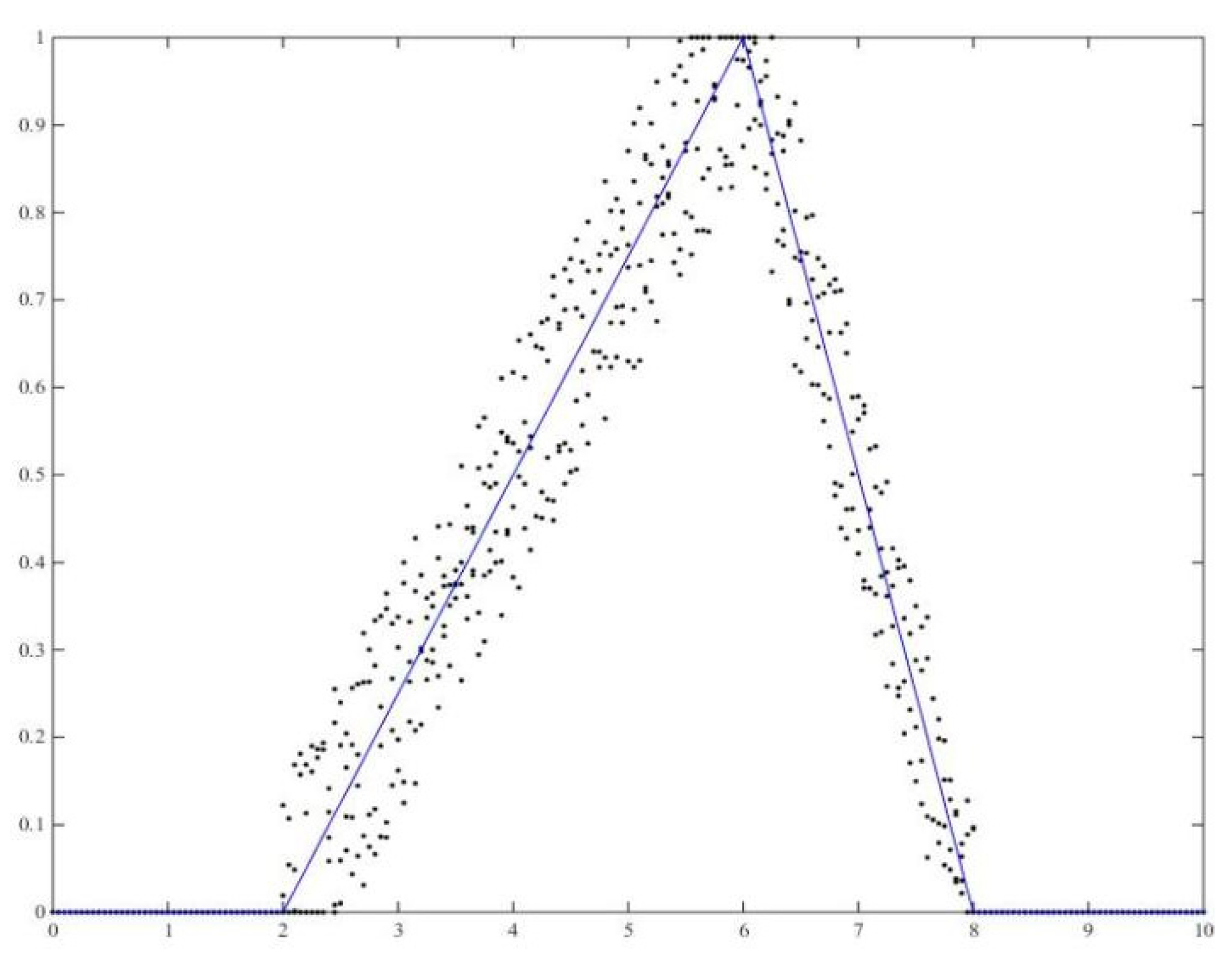
Example 2.

The hesitant possibility distribution${\mu }_{\xi }(t)$of triangle hesitant fuzzy variable$\xi$.

$$\frac{{\displaystyle {\sum }_{x\in {\mu }_{\xi }(t)}x}}{\text{\#}{\mu }_{\xi }(t)}=\{\begin{array}{cc}\frac{t-t_1}{t_2-t_1}& t_1\le t<t_2\\ \frac{t_3-t}{t_3-t_2}& t_2\le t<t_3\\ 0& else\end{array}$$

where$t_1<t_2<t_3$, and is shorthand for${\left(t_1,t_2,t_3\right)}_H$. For instance, the hesitant possibility distribution of${\left(2,6,8\right)}_H$is showed inFigure 1.

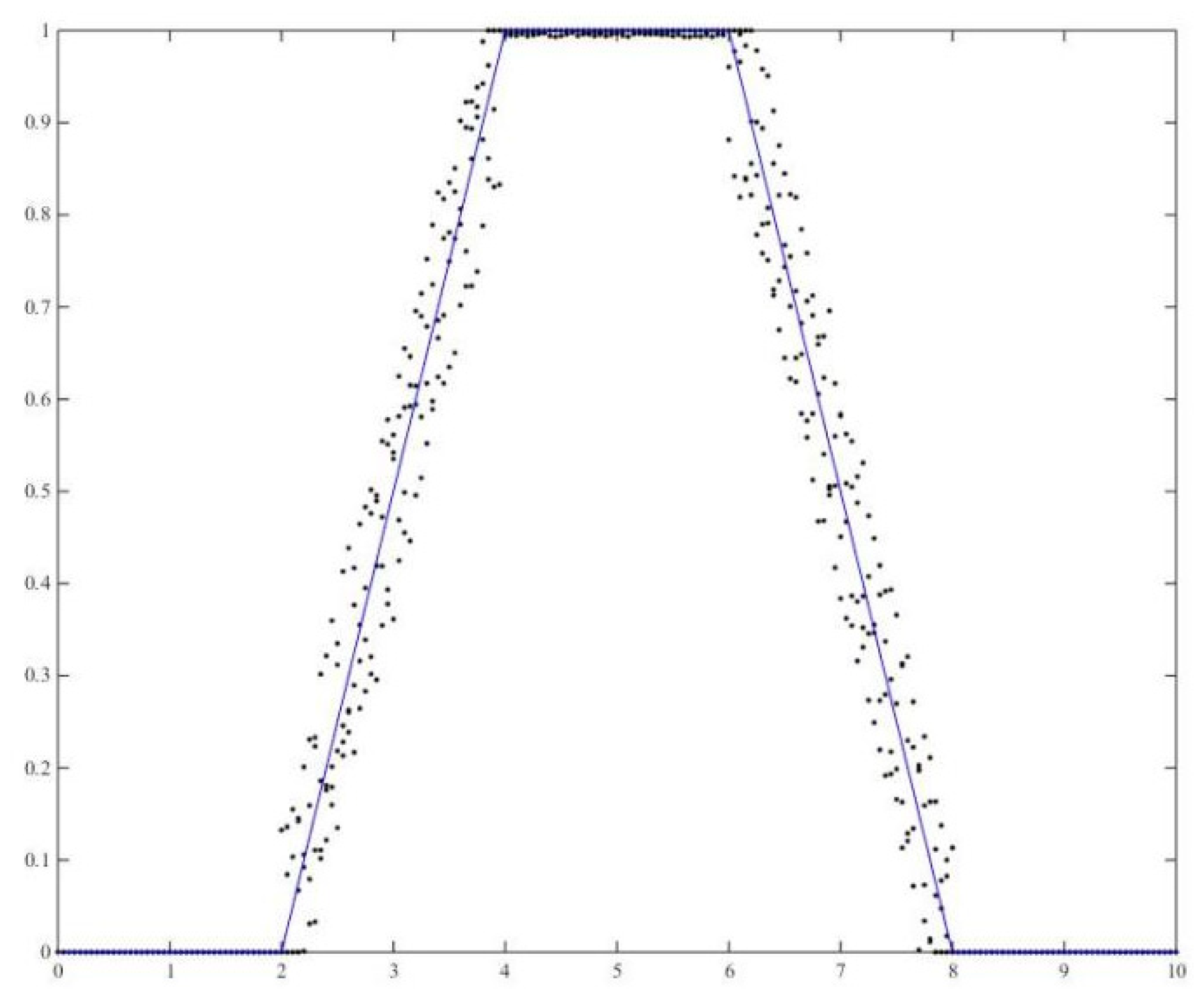
Example 3.

The hesitant possibility distribution${\mu }_{\xi }(t)$of the trapezoidal hesitant fuzzy variable$\xi$.

$$\frac{{\displaystyle {\sum }_{x\in {\mu }_{\xi }(t)}x}}{\text{\#}{\mu }_{\xi }(t)}=\{\begin{array}{cc}\frac{t-t_1}{t_2-t_1}& t_1\le t<t_2\\ 1& t_2\le t<t_3\\ \frac{t_4-t}{t_4-t_3}& t_3\le t<t_4\\ 0& else\end{array}$$

where$t_1<t_2<t_3<t_4$, and is shorthand for${\left(t_1,t_2,t_3,t_4\right)}_H$. For instance, the hesitant possibility distribution of${\left(2,4,6,8\right)}_H$is showed inFigure 2.

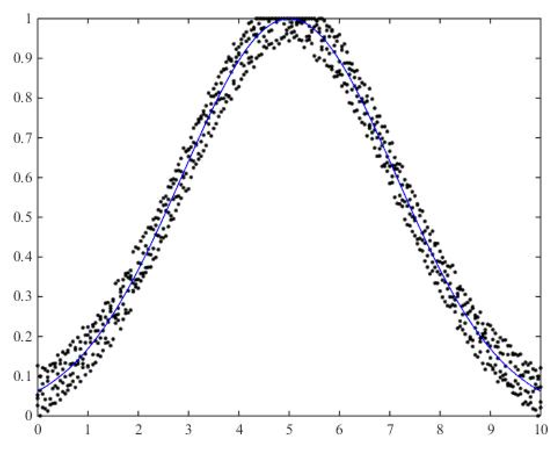
Example 4.

The hesitant possibility distribution${\mu }_{\xi }(t)$of the normal hesitant fuzzy variable$\xi$.

$$\frac{{\displaystyle {\sum }_{x\in {\mu }_{\xi }(t)}x}}{\text{\#}{\mu }_{\xi }(t)}=e^{\left\{-\frac{{(t-\alpha )}^2}{{\sigma }^2}\right\}}=\exp \left\{-{(t-\alpha )}^2/{\sigma }^2\right\}t\in \mathcal{R}$$

where$\alpha \in \mathcal{R},\sigma >0$, and is shorthand for$\left(\alpha ,{\sigma }^2\right)$. For instance, the hesitant possibility distribution of$\left(5,3^2\right)$is showed inFigure 3.

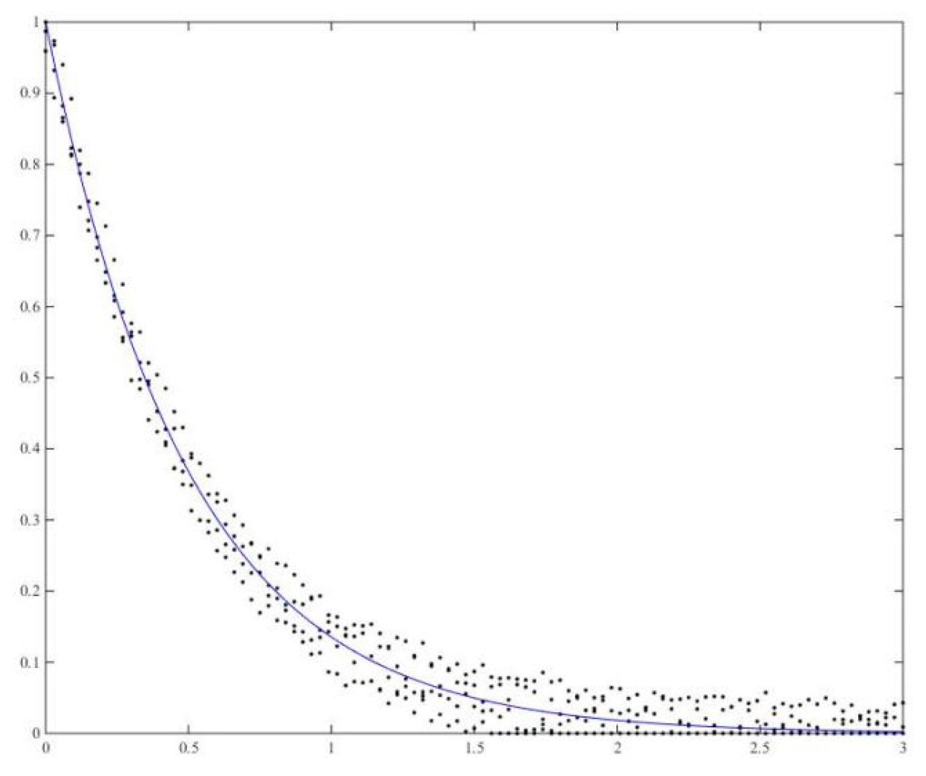
Example 5.

The hesitant possibility distribution${\mu }_{\xi }(t)$of the exponential hesitant fuzzy variable$\xi$.

$$\frac{{\displaystyle {\sum }_{x\in {\mu }_{\xi }(t)}x}}{\text{\#}{\mu }_{\xi }(t)}=e^{-\lambda t}=\exp \left\{-\lambda t\right\}t\in {\mathcal{R}}^{+}$$

where$\lambda >0$, and is shorthand for$\lambda$. For instance, the hesitant possibility distribution of$\lambda =2$is showed inFigure 4.

3.4. The Distribution of Functions of Hesitant Fuzzy Variable and the Distribution of Sum of Hesitant Fuzzy Variables

Theorem 12.

Provided that$(\Gamma ,\mathcal{A},Po{s}_H)$is a hesitant possibility measure space,$\xi$is a hesitant fuzzy variable, and$g$is a real-valued function; then,$g(\xi )$is also a hesitant fuzzy variable, and its hesitant possibility distribution is presented as follows.

$${\mu }_{g(\xi )}(x)=\left\{\underset{u\in g^{-1}(x)}{\sup }\left\{x_u\right\}|x_u\in {\mu }_{\xi }(u),u\in g^{-1}(x)\right\}$$

Proof. 

From the above conditions, we had

$$g(\xi ):\Gamma \to \mathcal{R},\mathrm{and}\left\{g(\xi )=x\right\}={\displaystyle {\cup }_{u\in g^{-1}(x)}\{\xi =u}\}\subset \mathcal{A}.$$

Therefore, $g(\xi )$ was a hesitant fuzzy variable; thus,

$$\begin{array}{l}{\mu }_{g(\xi )}(x)=Po{s}_H\left\{g(\xi )=x\right\}=Po{s}_H\left\{{\displaystyle {\cup }_{u\in g^{-1}(x)}\{\xi =u}\}\right\}\\ =\left\{\underset{u\in g^{-1}(x)}{\sup }\left\{x_u\right\}|x_u\in Po{s}_H\{\xi =U\},u\in g^{-1}(x)\right\}\\ =\left\{\underset{u\in g^{-1}(x)}{\sup }\left\{x_u\right\}|x_u\in {\mu }_{\xi }(u),u\in g^{-1}(x)\right\}\end{array}$$

□

Theorem 13.

Supposing that$(\Gamma ,\mathcal{A},Po{s}_H)$is a hesitant possibility measure space,$\xi$and$\eta$are mutually independent hesitant fuzzy variables, then$\xi +\eta$is also a hesitant fuzzy variable, and its hesitant possibility distribution is presented as follows.

$${\mu }_{\xi +\eta }(z)=\left\{\underset{x}{\sup }\left\{u\right\}|u\in \left\{u_1\wedge u_2|\begin{array}{l}{u}_1\in {\mu }_{\xi }(x)\\ u_2\in {\mu }_{\eta }(z-x)\end{array}\right\}\right\}$$

Proof. 

According to conditions, we obtained $\xi +\eta :\Gamma \to \mathcal{R}$ and

$$\left\{\xi +\eta =z\right\}=\left\{\left\{\xi +\eta =z\right\}\cap \Gamma \right\}=\left\{\left\{\xi +\eta =z\right\}\cap {\displaystyle \underset{x}{\cup }\left\{\xi =x\right\}}\right\}={\displaystyle \underset{x}{\cup }\left\{\xi =x,\xi +\eta =z\right\}}\subset \mathcal{A}.$$

Therefore, $\xi +\eta$ is a hesitant fuzzy variable; thus,

$$\begin{array}{ll}Po{s}_H\left\{\xi +\eta =z\right\}& =Po{s}_H\left\{\left\{\xi +\eta =z\right\}\cap \Gamma \right\}=Po{s}_H\left\{\left\{\xi +\eta =z\right\}\cap {\displaystyle \underset{x}{\cup }\left\{\xi =x\right\}}\right\}\\ & =Po{s}_H\left\{{\displaystyle \underset{x}{\cup }\left\{\xi =x,\xi +\eta =z\right\}}\right\}=Po{s}_H\left\{{\displaystyle \underset{x}{\cup }\left\{\xi =x,\eta =z-\xi \right\}}\right\}\\ & =\left\{\underset{x}{\sup }\left\{u\right\}|u\in Po{s}_H\left\{\xi =x,\eta =z-\xi \right\}\right\}\\ & =\left\{\underset{x}{\sup }\left\{u\right\}|u\in \left\{u_1\wedge u_2|\begin{array}{l}{u}_1\in Po{s}_H\left\{\xi =x\right\}\\ u_2\in Po{s}_H\left\{\eta =z-\xi \right\}\end{array}\right\}\right\}\\ & =\left\{\underset{x}{\sup }\left\{u\right\}|u\in \left\{u_1\wedge u_2|\begin{array}{l}{u}_1\in {\mu }_{\xi }(x)\\ u_2\in {\mu }_{\eta }(z-x)\end{array}\right\}\right\}\end{array}$$

□

4. Application of Hesitant Fuzzy Variables

In this section, we introduced two examples to show how hesitant fuzziness can be used to model for hesitant fuzzy graph and hesitant fuzzy group decision making.

4.1. Hesitant Fuzzy Graph Based on Hesitant Fuzzy Variable

The complexity of thinking and the cognitive differences among people have determined that it is difficult for people to reach an agreement on the same issue, they often have different views and, finally, they show a hesitant state. How can we more objectively reflect people’s different preferences and hesitations, and how close can we come to the real thinking mode of human beings. References [37,38,39,40] utilize the hesitant fuzzy set to describe the degree of hesitation in the human thinking process, while this paper, from another perspective, shows people’s hesitation more flexibly. This section mainly discussed the application of the hesitant fuzzy variable in simulating human subjective thinking and proposed a hesitant fuzzy graph according to the hesitant fuzzy variable.

Definition 14.

Suppose that$G=\left(V,E\right)$is a graph,$V=\{v_1,v_2,\cdots ,v_n\}$is a vertex set of the graph$G$,$E=\left\{e_{ij}\right\}$is an edge collection,$\left(V\times V,\mathcal{P}(V\times V),Po{s}_H\right)$is the hesitant possibility measure space and${\xi }_{ij}$is a hesitant fuzzy variable on$\left(V\times V,\mathcal{P}(V\times V),Po{s}_H\right)$. If edges$e_{ij}$of the graph$G=\left(V,E\right)$are presented by${\xi }_{ij}$,$G=\left(V,E\right)$is called the hesitant fuzzy graph, which is shorthand for$G=\left(V,E_{\xi },Po{s}_H\right)$.

From the above definition, the hesitant fuzzy variables show the existence and the hesitant fuzzy degree of vertexes and, in this sense, it can more objectively simulate the hesitant fuzzy degree in people’s thinking process. When ${\xi }_{ij}=1$, it explains that there is an edge $e_{ij}$ and its hesitant possibility is $Po{s}_H\{{\xi }_{ij}=1\}\in \mathcal{P}([0,1])$; when ${\xi }_{ij}=0$, it explains that there is no edge $e_{ij}$, and its hesitant possibility is $Po{s}_H\{{\xi }_{ij}=0\}\in \mathcal{P}([0,1])$.

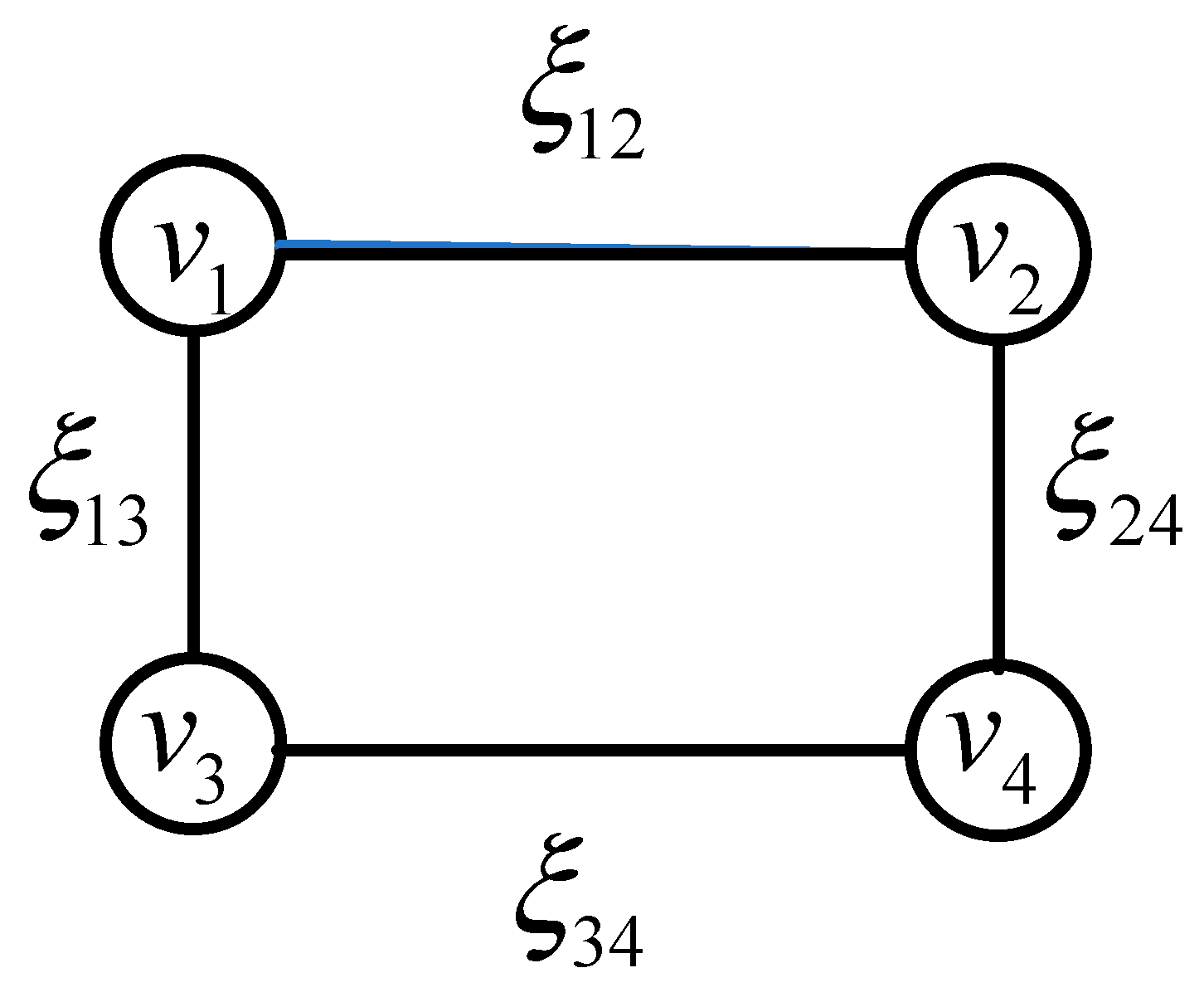
Therefore, a hesitant fuzzy graph consists of two components, the first one being the topological structure of the graph and the other one being the distribution table of the hesitant fuzzy variables corresponding to edges. For instance, Figure 5 shows the topology of a hesitant fuzzy graph, and

Table 1. The possibility and credibility distribution table of hesitant fuzzy graph.

Hesitant Fuzzy Distribution	Value	${\mathit{\xi }}_{12}$	${\mathit{\xi }}_{13}$	${\mathit{\xi }}_{24}$	${\mathit{\xi }}_{34}$
Hesitant possibility distribution	1	{0.8,0.9}	{0.2,0.3}	{1}	{0.6,0.7}
	0	{1}	{1}	{0.3,0.4,0.45}	{1}
Hesitant credibility distribution	1	{0.4,0.45}	{0.1,0.15}	{0.7,0.8,0.85}	{0.3,0.35}
	0	{0.55,0.6}	{0.85,0.9}	{0.15,0.2,0.225}	{0.5,0.7}

shows the distribution table of the related hesitation possibility and hesitation credibility.

4.2. Group Decision Making Based on Hesitant Fuzzy Variable

It could be potentially significant to describe a subjective opinion with hesitation by using hesitant fuzzy modelling. One of the most general situations is that a clear opinion of an individual is not necessarily on a practical question, but their hesitant feeling is stronger than others. In this sense, an individual’s hesitant judgement about an issue may be characterized by a hesitant fuzzy variable. As an example, a company manager may want to determine a collective opinion of his subordinates in regards to the quantity of allocated money, which applies to research and development activities. Let ${\xi }_i$ = {number of money the subordinate $i$ should be put into research and development activities}. The hesitant possible distributions of ${\xi }_i$$(i=1,2,3,4,5,6)$ might be as follows.

$${\mu }_{{\xi }_1}(x)=\{\begin{array}{cc}\{0.05,0.1\}& x\le \mathrm{200,000}\\ \{0.1,0.2\}& \mathrm{200,000}<x\le \mathrm{400,000}\\ \{0.2,0.3,0.4,\}& \mathrm{400,000}<x\le \mathrm{550,000}\\ \{0.8,0.9,1.0\}& \mathrm{550,000}<x\le \mathrm{700,000}\\ \{0.3,0.4\}& \mathrm{700,000}<x\le \mathrm{900,000}\\ \{0.0,0.05\}& \mathrm{900,000}<x\end{array}$$

$${\mu }_{{\xi }_2}(x)=\{\begin{array}{cc}\{0.02,0.05\}& x\le \mathrm{150,000}\\ \{0.2,0.3\}& \mathrm{150,000}<x\le \mathrm{350,000}\\ \{0.3,0.4,0.5,\}& \mathrm{350,000}<x\le \mathrm{500,000}\\ \{0.7,0.9,1.0\}& \mathrm{500,000}<x\le \mathrm{650,000}\\ \{0.2,0.4,0.5\}& \mathrm{650,000}<x\le \mathrm{850,000}\\ \{0.0,0.02\}& \mathrm{850,000}<x\end{array}$$

$${\mu }_{{\xi }_3}(x)=\{\begin{array}{cc}\{0.0,0.05\}& x\le \mathrm{100,000}\\ \{0.1,0.3\}& \mathrm{100,000}<x\le \mathrm{200,000}\\ \{0.3,0.5,\}& \mathrm{200,000}<x\le \mathrm{400,000}\\ \{0.8,1.0\}& \mathrm{400,000}<x\le \mathrm{700,000}\\ \{0.1,0.2,0.4\}& \mathrm{700,000}<x\le \mathrm{800,000}\\ \left\{0.0\right\}& \mathrm{800,000}<x\end{array}$$

$${\mu }_{{\xi }_4}(x)=\{\begin{array}{cc}\{0.05,0.15\}& x\le \mathrm{250,000}\\ \{0.1,0.3\}& \mathrm{250,000}<x\le \mathrm{350,000}\\ \{0.2,0.4,0.5,\}& \mathrm{350,000}<x\le \mathrm{550,000}\\ \{0.7,0.8,1.0\}& \mathrm{550,000}<x\le \mathrm{750,000}\\ \{0.4,0.5\}& \mathrm{750,000}<x\le \mathrm{850,000}\\ \left\{0.02\right\}& \mathrm{850,000}<x\end{array}$$

$${\mu }_{{\xi }_5}(x)=\{\begin{array}{cc}\left\{0.05\right\}& x\le \mathrm{100,000}\\ \{0.2,0.3\}& \mathrm{100,000}<x\le \mathrm{250,000}\\ \{0.3,0.4\}& \mathrm{250,000}<x\le \mathrm{450,000}\\ \{0.7,0.9\}& \mathrm{450,000}<x\le \mathrm{650,000}\\ \{0.2,0.3,0.5\}& \mathrm{650,000}<x\le \mathrm{800,000}\\ \{0.0,0.02\}& \mathrm{800,000}<x\end{array}$$

$${\mu }_{{\xi }_6}(x)=\{\begin{array}{cc}\left\{0.05\right\}& x\le \mathrm{160,000}\\ \{0.2,0.3\}& \mathrm{160,000}<x\le \mathrm{280,000}\\ \{0.3,0.4\}& \mathrm{280,000}<x\le \mathrm{480,000}\\ \{0.7,0.9\}& \mathrm{480,000}<x\le \mathrm{680,000}\\ \{0.2,0.3,0.5\}& \mathrm{680,000}<x\le \mathrm{880,000}\\ \{0.0,0.02\}& \mathrm{880,000}<x\end{array}$$

Now, suppose that a manager obtained the hesitant possible distribution describing the opinion of each subordinate, which is represented by a hesitant fuzzy variable. The question we deal with is the following: is there a way of making an inference for the hesitant possible distribution of a hesitant fuzzy variable associated with the group opinion from the hesitant possible distributions of hesitant fuzzy variables corresponding to the issues of each subordinate? Where the group opinion is only modeled except for an interactive group decision, we could assume that there are six constants ${\alpha }_1,{\alpha }_2,{\alpha }_3,{\alpha }_4,{\alpha }_5,{\alpha }_6$ with ${\displaystyle {\sum }_{i=1}^6{\alpha }_i}=1$, and ${\alpha }_i$ represent the importance of the $i$th subordinate’s opinion about the group opinion. For instance, when ${\alpha }_1=0.15$ and ${\alpha }_2=0.45$, the opinion of the second subordinate is three times more important than the first. We present that the hesitant fuzzy variable $\eta ={\displaystyle {\sum }_{i=1}^6{\alpha }_i{\xi }_i}$ is a reasonable explanation of the group opinion. As a result, the hesitant possible distribution of $\eta$ would be inferred by the following steps based on the hesitant possible distributions of $({\xi }_1,{\xi }_2,{\xi }_3,{\xi }_4,{\xi }_5,{\xi }_6)$.

(1)

Calculate the hesitant possible distribution of ${\alpha }_1{\xi }_1$, denoted as ${\mu }_{{\alpha }_1{\xi }_1}(x)$.

(2)

Compute the hesitant possible distribution of ${\alpha }_1{\xi }_1+{\alpha }_2{\xi }_2$ by the given operation in Theorem 13.

(3)

Sequentially perform the operation in the second step for the hesitant possible distribution of ${\alpha }_1{\xi }_1+{\alpha }_2{\xi }_2+{\alpha }_3{\xi }_3+{\alpha }_4{\xi }_4+{\alpha }_5{\xi }_5+{\alpha }_6{\xi }_6$.

(4)

According to the above, Theorem 4.1 and from the hesitant possible distribution of $\eta$, the hesitant possibility of $\{r_1<\eta \le r_2\}$ can be easily inferred for any $-\infty <r_1<+\infty ,-\infty <r_2<+\infty$. where $\{r_1<\eta \le r_2\}$ may represent the final opinion of a manager.

Although the introduced example is only a rough description of an application of the hesitant fuzzy variable in a group decision-making framework, it showed that the hesitant fuzzy variable concept appears to be convenient for modelling hesitant fuzzy decision-making problems.

5. Conclusions

This paper introduced the hesitant possibility measure, hesitant necessity measure and hesitant credibility measure on an ample space $(\Gamma ,\mathcal{A})$, and discussed some properties concerning these three set-valued measures, which, respectively, corresponded to the hesitant possibility measure space, hesitant necessity measure space and hesitant credibility measure space. On the hesitant fuzzy possibility measure space, a hesitant fuzzy variable was defined. Consequently, the distribution of this variable and one of its functions were introduced, including several common hesitant fuzzy variables such as the triangle hesitant fuzzy variable, trapezoid hesitant fuzzy variable, normal hesitant fuzzy variable and exponential hesitant fuzzy variable. As a result, the axiomatic system with regard to the hesitant possibility of hesitant fuzzy events was constructed. This axiomatic framework was based on the hesitant fuzzy variable and could provide theoretical support for hesitant fuzzy information processing, which was illustrated by two practical applications in the fourth section of this paper. In the future, according to obtained results of the hesitant fuzzy variable, the hesitant fuzzy theory could be enriched in digital numerical characteristics of the hesitant fuzzy variable such as the mathematical expectation, variance, correlation coefficient, covariance and all sorts of moments. Besides these notions, the multidimensional hesitant fuzzy variable and its distribution are also directions of further research in the future.

References

- Zadeh, L.A. Fuzzy sets. Inf. Control 1965, 8, 338–353. [Google Scholar] [CrossRef] [Green Version]
- Torra, V. Hesitant fuzzy sets. Int. J. Intell. Syst. 2010, 25, 529–539. [Google Scholar] [CrossRef]
- Alcantud, J.C.R.; Torra, V. Decomposition theorems and extension principles for hesitant fuzzy sets. Inf. Fusion 2018, 41, 48–56. [Google Scholar] [CrossRef]
- Xia, M.M.; Xu, Z.S. Hesitant fuzzy information aggregation in decision making. Int. J. Approx. Reason. 2011, 52, 395–407. [Google Scholar] [CrossRef] [Green Version]
- Xu, Z.S.; Xia, M.M. On Distance and Correlation Measures of Hesitant Fuzzy Information. Int. J. Intell. Syst. 2011, 26, 410–425. [Google Scholar] [CrossRef]
- Xu, Z.S.; Xia, M.M. Distance and similarity measures for hesitant fuzzy sets. Inf. Sci. 2011, 181, 2128–2138. [Google Scholar] [CrossRef]
- Xia, M.M.; Xu, Z.S. Managing hesitant information GDM problems under fuzzy and multiplicative preference relations. Int. J. Uncertain. Fuzz. 2013, 21, 865–897. [Google Scholar] [CrossRef]
- Zhang, Z.M.; Wang, C.; Tian, X.D. A decision support model for group decision making with hesitant fuzzy preference relations. Knowl.-Based Syst. 2015, 86, 77–101. [Google Scholar] [CrossRef]
- Zhang, Z.M.; Wang, C.; Tian, X.D. Multi-criteria group decision making with incomplete hesitant fuzzy preference relations. Appl. Soft. Comput. 2015, 36, 1–23. [Google Scholar] [CrossRef]
- Zhu, B.; Xu, Z.S. Probability-hesitant fuzzy sets and the representation of preference relations. Technol. Econ. Dev. Eco. 2018, 24, 1029–1040. [Google Scholar] [CrossRef]
- Xu, Y.J.; Cabrerizo, F.J.; Herrera-Viedma, N. A consensus model for hesitant fuzzy preference relations and its application in water allocation management. Appl. Soft. Comput. 2017, 58, 265–284. [Google Scholar] [CrossRef]
- Liao, H.C.; Xu, Z.S. Some new hybrid weighted aggregation operators under hesitant fuzzy multi-criteria decision making environment. J. Intell. Fuzzy Syst. 2014, 26, 1601–1617. [Google Scholar] [CrossRef]
- Zhao, N.; Xu, Z.S.; Ren, Z.L. On typical hesitant fuzzy prioritized or operator in multi-attribute decision making. Int. J. Intell. Syst. 2015, 31, 73–100. [Google Scholar] [CrossRef]
- Meng, F.Y.; Chen, X.H.; Zhang, Q. Induced generalized hesitant fuzzy Shapley hybrid operators and their application in multi-attribute decision making. Appl. Soft. Comput. 2015, 28, 599–607. [Google Scholar] [CrossRef]
- Tan, C.Q.; Yi, W.T.; Chen, X.H. Hesitant fuzzy Hamacher aggregation operators for multicriteria decision making. Appl. Soft. Comput. 2015, 26, 325–349. [Google Scholar] [CrossRef]
- Qin, J.D.; Liu, X.W.; Pedrycy, W. Frank aggregation operators and their application to hesitant fuzzy multiple attribute decision making. Appl. Soft Comput. 2016, 41, 428–452. [Google Scholar] [CrossRef]
- Riaz, M.; Batool, S.; Almalki, Y.; Ahmad, D. Topological Data Analysis with Cubic Hesitant Fuzzy TOPSIS Approach. Symmetry 2022, 14, 865. [Google Scholar] [CrossRef]
- Akram, M.; Adeel, A.; Alcantud, J.C.R. Multi-criteria group decision-making using an m-polar hesitant fuzzy TOPSIS approach. Symmetry 2019, 6, 795. [Google Scholar] [CrossRef] [Green Version]
- Chen, L.; Xu, H.; Ke, G.Y. A PROMETHEE II Approach Based on Probabilistic Hesitant Fuzzy Linguistic Information with Applications to Multi-Criteria Group Decision-Making. Int. J. Fuzzy Syst. 2021, 23, 1556–1580. [Google Scholar] [CrossRef]
- Akram, M.; Adeel, A.; Al-Kenani, A.N.; Alcantud, J.C.R. Hesitant fuzzy N-soft ELECTRE-II model: A new framework for decision-making. Neural Comput. Appl. 2021, 33, 7505–7520. [Google Scholar] [CrossRef]
- Krishankumar, R.; Ravichandran, K.S.; Kar, S.; Gupta, P.; Mehlawat, M.K. Double-hierarchy hesitant fuzzy linguistic term set-based decision framework for multi-attribute group decision-making. Soft Comput. 2021, 25, 2665–2685. [Google Scholar] [CrossRef]
- Liu, P.; Shen, M.; Teng, F.; Zhu, B.; Rong, L.; Geng, Y. Double hierarchy hesitant fuzzy linguistic entropy-based TODIM approach using evidential theory. Inf. Sci. 2021, 547, 223–243. [Google Scholar] [CrossRef]
- Liu, P.; Pan, Q.; Xu, H.; Zhu, B. An Extended QUALIFLEX Method with Comprehensive Weight for Green Supplier Selection in Normal q-Rung Orthopair Fuzzy Environment. Int. J. Fuzzy Syst. 2022, 1, 1–29. [Google Scholar] [CrossRef]
- Akram, M.; Adeel, A.; Alcantud, J.C.R. Group decision-making methods based on hesitant N-soft sets. Exper. Syst. Appl. 2019, 115, 95–105. [Google Scholar] [CrossRef]
- Alcantud, J.C.R.; Giarlotta, A. Necessary and possible hesitant fuzzy sets: A novel model for group decision making. Inf. Fusion 2019, 46, 63–76. [Google Scholar] [CrossRef]
- Alcantud, J.C.R.; Santos-García, G.; Peng, X.; Zhan, J. Dual extended hesitant fuzzy sets. Symmetry 2019, 5, 714. [Google Scholar] [CrossRef] [Green Version]
- Akram, M.; Adeel, A.; Alcantud, J.C.R. Hesitant fuzzy N-soft sets: A new model with applications in decision-making. J. Intell. Fuzzy Syst. 2019, 6, 6113–6127. [Google Scholar] [CrossRef]
- Yu, Q.; Li, Y.; Cao, J.; Hou, F. QUALIFLEX and LINMAP-based Approach for Multi-attribute Decision Making Problems with Simplified Neutrosophic Hesitant Fuzzy Sets. Opera. Res. Manag. Sci. 2021, 30, 77. [Google Scholar]
- Pierre, B. Probability Theory and Stochastic Processes; Springer: Cham, Switzerland, 2020; pp. 37–39. [Google Scholar]
- Liu, Y.K. Credibility Measure Theory; Science press: Beijing, China, 2018; pp. 4–11. [Google Scholar]
- Liu, Y.K.; Liu, B.D. A class of fuzzy random optimization: Expected value models. Inf. Sci. 2003, 155, 89–102. [Google Scholar] [CrossRef]
- Nahmias, S. Fuzzy variables. Fuzzy Set. Syst. 1978, 1, 97–110. [Google Scholar] [CrossRef]
- Wang, P.Z. Fuzzy contactibility and fuzzy variables. Fuzzy Set. Syst. 1982, 8, 81–92. [Google Scholar] [CrossRef]
- Grabisch, M. Fuzzy integral in multicriteria decision making. Fuzzy Set. Syst. 1995, 69, 279–298. [Google Scholar] [CrossRef]
- Mesiar, R. Fuzzy measures and integrals. Fuzzy Set. Syst. 2005, 156, 365–370. [Google Scholar] [CrossRef]
- Khaista, R.; Saleem, A. Some new generalized interval-valued Pythagorean fuzzy aggregation operators using Einstein t-norm and t-conorm. Int. J. Intell. Syst. 2019, 37, 1–22. [Google Scholar]
- Peng, D.H.; Yang, K.D. A TOPSIS method in completely hesitant fuzzy environment. Fuzzy Syst. Math. 2018, 32, 39–50. [Google Scholar]
- Lv, J.h.; Guo, S.Z. Hesitant Fuzzy Group Decision Making Under Incomplete Information. Fuzzy Syst. Math. 2017, 31, 100–107. [Google Scholar]
- Zhang, C.; Li, D. Hesitant fuzzy graph and its application in multi-attribute decision making. Int. J. Patran. Recogn. 2017, 30, 1012–1018. [Google Scholar]
- Karaaslan, F. Hesitant fuzzy graphs and their applications in decision making. J. Intell. Fuzzy Syst. 2018, 36, 1–13. [Google Scholar] [CrossRef]
Figure 1.
Hesitant possibility distribution map of .
Figure 2.
Figure 3.
Figure 4.
Figure 5.
A hesitant fuzzy graph containing 4 vertexes.