Dynamic Event-Triggered Integral Sliding Mode Adaptive Optimal Tracking Control for Uncertain Nonlinear Systems

Abstract

In this paper, we study the event-triggered integral sliding mode optimal tracking problem of nonlinear systems with matched and unmatched disturbances. The goal is to design an adaptive dynamic programming-based sliding-mode controller, which stabilizes the closed-loop system and guarantees the optimal performance of the sliding-mode dynamics. First, in order to remove the effects of the matched uncertainties, an event-triggered sliding mode controller is designed to force the state of the systems on the sliding mode surface without Zeno behavior. Second, another event-triggered controller is designed to suppress unmatched disturbances with a nearly optimal performance while also guaranteeing Zeno-free behavior. Finally, the benefits of the proposed algorithm are shown in comparison to several traditional triggering and learning-based mechanisms.

1. Introduction

Traditional control systems are implemented with time-triggered (TT) sampling (i.e., periodic sampling). Data are sent from the controller to the actuator (or from the sensor to the controller) using a fixed sample length. However, in modern control systems, especially networked control systems, control signals are often implemented aperiodically [1]. The advantages of the aperiodic sampling in terms of update times have been elaborated in [2] in detail. In fact, the limited communication bandwidth in networked control systems has stimulated a huge attention in event-triggered control (ETC) [3,4,5,6,7,8,9,10,11], as an alternative to TT. Despite the progress in the filed, some problems remain open, such as how to simultaneously counteract the effect of matched and unmatched disturbances while guaranteeing the optimal performance of the ETC systems, which is one of our concerns and is an issue to be studied.

Owing to the distinguished features such as fast dynamic response, robustness, order reduction, and implementation simplicity, sliding mode control (SMC) is widely studied in the fields of transportation, power grid, industrial communication networks, and uncertain serial industrial robots [12,13,14,15,16,17,18,19,20]. Especially, SMC has been recognized as one of the popular and powerful control tools in power converters based on deriving from the variable structure systems theorem. In addition, its popularity comes from the robustness feature, which eliminates the burden of the necessity of system parameters required for accurate modeling, yet it may lack robustness against unmatched disturbances. Although many achievements in codesign of sliding mode control and event-triggered have emerged [21,22,23], they all neglect how to guarantee the optimal performance of the controlled system in the presence of matched and unmatched disturbances.

Optimal control theory is now quite mature [24,25,26,27]. Optimal control for nonlinear systems requires one to solve the Hamilton–Jacobi–Bellman (HJB) or Hamilton–Jacobi–Isaac (HJI) equations. However, the nonlinearity of the above equation makes it impossible to get an analytical solution [28]. Although numerical solutions via dynamic programming [29] can be obtained, issues of offline optimization and curse of dimensionality make these numerical methods not feasible in practical applications. To address these shortcomings, adaptive dynamic programming (ADP), oriented from reinforcement learning (RL) technique, has been widely researched in recent decades [30,31,32,33,34,35].

Event-triggered ADP [36,37,38] and event-triggered ADP-based ISMC [39,40] have been investigated in the past years. However, some open issues still remain, which are explained as follows. Although event-triggered implementations can reduce the update times of standard TT implementations, it needs to be pointed out that the event-triggering techniques developed in [39,40] depend only on the current state (static event-triggered control). It is well known that static event-triggered techniques may effectively reduce the communication cost when the sampling error is large. However, as the sampling error becomes smaller, this technique will become conservative, i.e., it can cause several unnecessary triggering. So, developing more flexible event-triggering conditions to further save resources is urgently needed. Moreover, it is still an open problem to design a learning-based event-triggered strategy while at the same time relaxing the excitation condition typically required for ADP methods to further reduce triggered times. Enlightened by the aforementioned discussions, in this article, we will provide a new learning-based framework for ETC-based ISM optimal tracking problem. The novelties are presented below.

• Different from the combined SMC and ADP frameworks of [39,40], this paper proposes a new dynamic event-triggered (DET) mechanism. By introducing an auxiliary variable, which is non-negative. This can increase the length of the time intervals between triggering events, further reducing the communication burden compared with [39,40].
• A novel Integral Sliding Mode Control (ISMC) scheme based on DET for uncertain nonlinear systems is proposed, consisting of two control laws. A first event-triggered controller is designed to tackle the matched uncertainties and force the trajectory of the system on the sliding mode surface. A second event-triggered controller is designed to tackle the unmatched uncertainties and guarantee optimal performance.
• To solve the resulting optimal control problem, a critic-only neural network (NN) based on ADP is proposed via the experience replay technique, which helps relaxing the excitation condition typically required for ADP methods to work. Stability of the closed-loop system is proven in the sense of uniformly ultimately boundedness, while guaranteeing Zeno-free behavior of the triggering mechanism.

The paper is arranged as follows. In Section 2, we introduce the model formulation and preliminaries. Section 3 covers the event-triggered-based ISMC design. Section 4 presents the framework of a dynamic triggered ADP strategy, along with stability analysis. Section 5 illustrates the effectiveness of the novel algorithm via comparative simulations. Section 6 gives the conclusions and possible future works.

Notations: ${\mathbb{R}}^{+}$ represents the sets of the positive real numbers. ${\mathbb{R}}^n$ and ${\mathbb{R}}^{n\times m}$ denote the space of all real n-vectors and the space of all $n\times m$ real matrices, respectively. ≜ means “equal by definition”, and $I_n$ is the identity matrix of dimension $n\times n$. T is the transposition symbol. ${\mathcal{C}}^1$ represents the class of functions with continuous derivative. ${\lambda }_{min}\left(X\right)$ is defined as the minimum eigenvalue of matrix X, $\parallel ·\parallel$ represents the 2-norm of a vector or matrix. For any full column rank matrix $\mathcal{F}(·)$, its left pseudoinverse is ${\mathcal{F}}^{†}(·)\triangleq {\left({\mathcal{F}}^T(·)\mathcal{F}(·)\right)}^{-1}{\mathcal{F}}^T(·)$.

2. System Formulation and Preliminaries

In this section, an ISMC design oriented toward optimal tracking is discussed. To target optimality, it is useful to introduce an augmented system associated with the tracking error system and the desired reference system.

Consider the following nonlinear system with matched and unmatched uncertainties [39]:

$$\dot{x}=p\left(x\right)+q\left(x\right)(u+d)+\overline{h}\left(x\right)\mathrm{w}$$

(1)

where $x\in {\mathbb{R}}^n$, $u\in {\mathbb{R}}^m$, $d\in {\mathbb{R}}^m$ and $\mathrm{w}\in {\mathbb{R}}^q$ are the system state, control input, unknown bounded matched disturbance, and unknown bounded unmatched disturbance, respectively. The system dynamics $p\left(x\right),q\left(x\right)$ and $\overline{h}\left(x\right)$ are known Lipschitz functions with $p\left(0\right)=0$, and $\parallel q\left(x\right)\parallel$ and $\parallel \overline{h}\left(x\right)\parallel$ having a positive upper bound. Meanwhile, let the system (1) be controllable, and the matrix function $q\left(x\right)$ be full column rank with $q(·)\ne \overline{h}(·)$.

Remark 1.

Herein, it should be noted that system (1) is favored by scholars in theoretical studies [18,33,35] as well as has been widely studied and explored in practical applications, such as a single link robot arm [39,40]; power system [34]; a spacecraft [41] et al.

The desired signal $x_d$ is subject to

$$\begin{array}{c}\hfill {\dot{x}}_d=r\left(x_d\right)\end{array}$$

(2)

where the bounded $x_d\in {\mathbb{R}}^n$ is Lipschitz continuous with $r\left(0\right)=0$. Define the tracking error

$$\begin{array}{c}\hfill e_d=x-x_d.\end{array}$$

(3)

Combining (1)–(3), $e_d$ satisfies the following dynamics

$$\begin{array}{c}\hfill {\dot{e}}_d=p\left(x\right)+q\left(x\right)(u+d)+\overline{h}\left(x\right)\mathrm{w}-{\dot{x}}_d.\end{array}$$

(4)

Define the augmented state $\xi ={[e_d^T,x_d^T]}^T\in {\mathbb{R}}^{2n}$. Combining (2) with (4) generates the following augmented system

$$\dot{\xi }=f\left(\xi \right)+g\left(\xi \right)(u+d)+h\left(\xi \right)\mathrm{w}$$

(5)

with

$$\begin{array}{cc}\hfill & f\left(\xi \right)=\left[\begin{array}{c}p(e_d+x_d)-r\left(x_d\right)\\ r\left(x_d\right)\end{array}\right]\hfill \\ \hfill & g\left(\xi \right)=\left[\begin{array}{c}q(e_d+x_d)\\ 0\end{array}\right]\hfill \\ \hfill & h\left(\xi \right)=\left[\begin{array}{c}\overline{h}(e_d+x_d)\\ 0\end{array}\right]\hfill \end{array}$$

where $f\left(\xi \right)\in {\mathbb{R}}^{2n}$, $g\left(\xi \right)\in {\mathbb{R}}^{2n\times m}$ and $h\left(\xi \right)\in {\mathbb{R}}^{2n\times q}$.

For simplicity and convenience of analysis, we will omit some arguments of the functions ($f\left(\xi \right),g\left(\xi \right),\mathrm{and}h\left(\xi \right)$ will be written as $f,g,\mathrm{and}h$, respectively) in the later part of the paper. To this end, the following two standard assumptions are required.

Assumption 1

([39]). System dynamics (5) with $f\left(0\right)=0$ is Lipschitz continuous, and $g\mathrm{and}h$ satisfy $\parallel g\parallel \le b_q(b_q\in {\mathbb{R}}^{+})$ and $\parallel h\parallel \le b_h(b_h\in {\mathbb{R}}^{+})$, respectively. The disturbances d and $\mathrm{w}$ satisfy $\parallel d\parallel \le b_d(b_d\in {\mathbb{R}}^{+})$ and $\parallel \mathrm{w}\parallel \le b_{\mathrm{w}}(b_{\mathrm{w}}\in {\mathbb{R}}^{+})$, respectively.

Assumption 2

([39]). The matrix function g is full column rank and its left pseudoinverse is given by $g^{†}={\left(g^{T}g\right)}^{-1}{g}^T$ and there exists some positive values $b_{q^{†}}(b_{q^{†}}\in {\mathbb{R}}^{+})$ such that $\parallel g^{†}\parallel \le b_{q^{†}}$. Then, the following equality holds

$$\begin{array}{c}\hfill h\mathrm{w}=g{g}^{†}h\mathrm{w}+(I-g{g}^{†})h\mathrm{w}\end{array}$$

(6)

where $\parallel g{g}^{†}h\parallel \le b_{g^{†}}(b_{g^{†}}\in {\mathbb{R}}^{+})$.

Control objective: This article aims to achieve an optimal tracking control of system state x for the desired trajectory $x_d$, so that the tracking error is uniformly ultimately bounded UUB. The control input should eliminate the effect of the matched disturbance and reduce the effects of the unmatched disturbance.

To achieve this goal, first, a new composite control law in the form $u=u_0+u_1$ will be considered. Second, according to the robustness to nonlinearities and uncertainties of SMC technique, the Section 3 designs an integral sliding surface and event-triggered controller $u_1$ aiming to suppress the matched effects of the systems while forcing the state of the systems on the sliding mode surface without Zeno-free behavior. Then, event-triggered optimal controller $u_0$ is designed aiming to reduce the unmatched effect and guarantee the optimal performance of the sliding-mode dynamics in Section 4. Finally, a nonlinear single link robot arm is considered to verify the effectiveness of the proposed algorithm.

3. DET-Based ISMC Design

To tackle the uncertainty affecting the nonlinear system (5), an integral type sliding surface is designed as

$$\begin{array}{cc}\hfill S\left(\xi \right)=& \mathcal{M}[\xi -{\xi }_0-{\int }_0^t\left(f+g{u}_0\right)\mathrm{d}\tau ]\hfill \end{array}$$

(7)

where $\mathcal{M}\in {\mathbb{R}}^{m\times 2n}(m<2n)$ is a projection matrix satisfying that $\mathcal{M}g$ is invertible. Here, $u_0$ is an optimal control input that will be designed in the next section. In this section, we aim to design the control $u_1$ to force the augmented system (5) onto the manifold $\left\{\xi \right|S(\xi ,t)=0\}$ in finite time, to remove the effect of matched disturbances. This can be achieved via

$$\begin{array}{c}\hfill u_1\left(t\right)=-\mathrm{X}\mathrm{sgn}\left(g^T{\mathcal{M}}^{T}S\left(\xi \right)\right)\end{array}$$

(8)

where $\mathrm{X}>0$. The sign function $\mathrm{sgn}(·)$ is

$$\mathrm{sgn}\left(\alpha \right)=\left\{\begin{array}{c}\hfill 1,\alpha >0,\\ \hfill 0,\alpha =0,\\ \hfill -1,\alpha <0.\end{array}\right.$$

Next, we introduce the dynamics of the sliding variable and the notion of practical sliding mode, which will be required later. The dynamics of the sliding variable can be obtained by differentiating (7) with respect to time

$$\begin{array}{c}\hfill \dot{S}\left(\xi \right)=\mathcal{M}[\dot{\xi }-(f+g{u}_0)].\end{array}$$

(9)

According to the SMC theory, when the system trajectories reach the manifold, one has $\dot{S}=0$. Then, by combining (5), (6) and (9), one has an equivalent control $u_{1eq}$ satisfying

$$\begin{array}{c}\hfill u_{1eq}=-d-g^{†}h\mathrm{w}-{\left(\mathcal{M}g\right)}^{-1}\mathcal{M}(I-g{g}^{†})h\mathrm{w}.\end{array}$$

(10)

Substituting the equivalent control (10) into the augmented system (5), one gets thew dynamics on the sliding manifold

$$\begin{array}{cc}\hfill \dot{\xi }& =f+g{u}_0+[I-g{\left(\mathcal{M}g\right)}^{-1}\mathcal{M}]{\mathrm{w}}_u\hfill \end{array}$$

(11)

where ${\mathrm{w}}_u=[I-g{g}^{†}]h\mathrm{w}$. The following result is recalled.

Lemma 1

([18]). The optimal solution to the following optimization problem

$$\begin{array}{c}\hfill \underset{\mathcal{M}\in {\mathbb{R}}^{m\times 2n}}{argmin}{\parallel [I-g{\left(\mathcal{M}g\right)}^{-1}\mathcal{M}]{\mathrm{w}}_u\parallel }_2\end{array}$$

is $\mathcal{M}=g^{†}$.

Remark 2.

Since $\mathcal{M}$ is the left pseudoinverse of g, one knows

(1) 

$\mathcal{M}=g^{†}$ can minimize ${\mathrm{w}}_{ueq}$, which leads to ${\mathrm{w}}_{ueq}={\mathrm{w}}_u$, refer to [18] for the detailed proof;

(2) 

The modulation gain associated with $u_1\left(t\right)$ is minimized, which means that the amplitude of chattering can be reduced;

(3) 

$\mathcal{M}=g^{†}$ avoids amplifying the effect of the unmatched disturbance.

To extend the continuous-time control $u_1$ in the event-triggered paradigm, we define a virtual control input $\mu \left(t\right)$ satisfying $\mu \left(t\right)\triangleq u\left(t_k\right),t\in [t_k,t_{k+1})$, where

$$\begin{array}{c}\hfill \mu \left(t\right)=-\mathrm{X}\mathrm{sgn}\left(g^T{\mathcal{M}}^{T}S\left(\xi \left(t_k\right)\right)\right)\end{array}$$

(12)

and ${\left\{t_k\right\}}_{k=0}^{\infty }$ is a sampling sequence with $t_k<t_{k+1},k\in \mathbb{N}$ with $\mathbb{N}=\{0,1,2,\cdots \}$. Define the following measurement error

$$\begin{array}{cc}\hfill e_{u_1}& =\mu \left(t_k\right)-\mu \left(t\right)\hfill \\ \hfill & =\mathrm{X}\mathrm{sgn}\left(g^T{\mathcal{M}}^{T}S\left(\xi \right)\right)-\mathrm{X}\mathrm{sgn}\left(g^T\left({\xi }_k\right){\mathcal{M}}^T\left({\xi }_k\right)S\left({\xi }_k\right)\right)\hfill \end{array}$$

(13)

satisfying the following triggering condition

$$\begin{array}{c}\hfill t_{k+1}=inf\{t>t_k|\mathrm{X}-b_d-b_{q^{†}}-\parallel e_{u_1}\left(t\right)\parallel \le 0\},t_0=0.\end{array}$$

(14)

The following theorem establishes a sufficient condition to the reachability of the specified sliding surface (7).

Theorem 1.

Suppose Assumptions 1 and 2 hold. Consider the augmented system (5) with the sliding surface (7) under event-triggered controller (12). Then, practical sliding mode is achieved if the triggering condition satisfies (14).

Proof. 

Consider the following Lyapunov function $V_1=\frac{1}{2}{S}^{T}S$. For $t\in [t_k,t_{k+1})$, the time derivative $V_1$ concerning system (5) with (12) is

$$\begin{array}{cc}\hfill {\dot{V}}_1& =S^T\dot{S}\hfill \\ \hfill & =S^T\mathcal{M}[\dot{\xi }-f-g{u}_0]\hfill \\ \hfill & =S^T\mathcal{M}[f+g(u_0\left(t_k\right)+u_1\left(t_k\right)+d)+h\mathrm{w}-(f+g{u}_0\left(t_k\right))]\hfill \\ \hfill & =S^T\mathcal{M}[g(u_1\left(t_k\right)+d+g^{†}h\mathrm{w})+{\mathrm{w}}_u]\hfill \\ \hfill & =S^T\mathcal{M}g[(e_{u_1}\left(t\right)-\mathrm{X}\mathrm{sgn}\left(g^T{\mathcal{M}}^{T}S\right)+d+g^{†}h\mathrm{w}]+S^T\mathcal{M}g{\left(\mathcal{M}g\right)}^{-1}\mathcal{M}{\mathrm{w}}_u\hfill \\ \hfill & \le \parallel S^T\mathcal{M}g\parallel [-\mathrm{X}+b_d+b_{q^{†}}+\parallel e_{u_1}\left(t\right)\parallel ]+\parallel S^T\mathcal{M}g{\left(\mathcal{M}g\right)}^{-1}\mathcal{M}{\mathrm{w}}_u\parallel .\hfill \end{array}$$

(15)

Substituting $\mathcal{M}=g^{†}$ into (15), we have ${\dot{V}}_1\le -\parallel S^T\parallel [\mathrm{X}-b_d-b_{q^{†}}-\parallel e_{u_1}\left(t\right)\parallel ].$ Noticing the triggering condition (14), we know that $\parallel e_{u_1}\parallel \le \mathrm{X}-b_d-b_{q^{†}}$ holds all the time, then ${\dot{V}}_1<0$ for $\parallel S\parallel \ne 0$, which implies that the system state $\xi$ starting from the initial state $\xi \left(0\right)$ slide robustly on the switching surface S from initial time $t=0$ and can gradually reach the sliding mode surface $S=0$. The proof is completed.    □

Theorem 2.

The event-triggered rule (14) avoids the Zeno behavior, since a minimal triggering interval is given by

$$T_{u_1}\left(k\right)\ge \frac{\nu (\mathrm{X}-b_d-b_{q^{†}})}{n\parallel \mathrm{X}\parallel (\parallel \mathrm{X}\parallel +b_d+b_{q^{†}})}.$$

Proof. 

Define $T_{u_1}\left(k\right)=t_{k+1}-t_k$ as the interexecution time for $u_1$. Recall that the control $u_1$ is updated at $t=t_k$ and $e_{u_1}\left(t_k\right)=0$. During the event intervals

$$\begin{array}{cc}\hfill \frac{d\parallel e_{u_1}\left(t\right)\parallel }{dt}& \le \parallel \frac{d{e}_{u_1}\left(t\right)}{dt}\parallel =\parallel \frac{d}{dt}[\mu \left(t\right)-u_1\left(t\right)]\parallel \hfill \\ \hfill & =\parallel \frac{d}{dt}[-\mathrm{X}\mathrm{sgn}\left(g^T\left({\xi }_k\right){\mathcal{M}}^T\left({\xi }_k\right)S\left({\xi }_k\right)\right)\hfill \\ \hfill & +\mathrm{X}\mathrm{sgn}\left(g^T\left(\xi \right){\mathcal{M}}^{T}S\left(\xi \right)\right)]\parallel \hfill \\ \hfill & \le \parallel \frac{d}{dt}\left[\mathrm{X}\mathrm{sgn}\left(g^T\left(\xi \right){\mathcal{M}}^{T}S\left(\xi \right)\right)\right]\parallel .\hfill \end{array}$$

(16)

The technique [39] is utilized to approximate the sign function $\mathrm{sgn}\left(S\right)$. That is, $\mathrm{sgn}\left(S\right)\approx \tanh (S/\nu )$ where $\nu \ge 1$. Substituting $\mathcal{M}=g^{†}$ into (16), we have

$$\begin{array}{cc}\hfill \frac{d\left|\right|e_{u_1}\left(t\right)\left|\right|}{dt}& \le \parallel \frac{d}{dt}[\mathrm{X}tanh\left(g^T\left(\xi \right){\mathcal{M}}^T\left(\xi \right)S\right)]\parallel \hfill \\ \hfill & =\parallel \mathrm{X}\parallel \parallel I_n-{tanh}^2\left(g^T\left(\xi \right){\mathcal{M}}^T\left(\xi \right)S\right)\parallel \parallel \frac{1}{\nu }\dot{S}\parallel .\hfill \end{array}$$

As $\parallel I_n-{tanh}^2\left(g^T\left(\xi \right){\mathcal{M}}^T\left(\xi \right)S\right)\parallel \le \parallel I_n\parallel =n$, using (7), we have

$$\begin{array}{cc}\hfill \frac{d\parallel e_{u_1}\left(t\right)\parallel }{dt}& \le (n/\nu )\parallel \mathrm{X}\parallel \parallel \mathcal{M}\parallel \parallel \dot{\xi }-[f+g{u}_0]\parallel \hfill \\ \hfill & \le (n/\nu )\parallel \mathrm{X}\parallel \parallel \mathcal{M}g\parallel \parallel u_1\left({\xi }_k\right)+d\left(t\right)+g^{†}k\mathrm{w}\parallel \hfill \\ \hfill & \le (n/\nu )\parallel \mathrm{X}\parallel (\parallel \mathrm{X}\parallel +b_d+b_{q^{†}}).\hfill \end{array}$$

(17)

After integrating both sides with respect to (17) for $t\in [t_k,t_{k+1})$, we get

$$\begin{array}{c}\hfill \parallel e_{u_1}\parallel \le (t-t_k)(n/\nu )\parallel \mathrm{X}\parallel (\parallel \mathrm{X}\parallel +b_d+b_{q^{†}}).\end{array}$$

(18)

Using the event-triggered rule (14), when $t\in [0,{\tau }_{\infty }),$ one has

$$\begin{array}{c}\hfill \left|\right|e_{u_1}\left|\right|\ge \mathrm{X}-b_d-b_{q^{†}}.\end{array}$$

(19)

For $\forall t\in [t_k,t_{k+1})$, there is $t-t_k\le t_{k+1}-t_k=T_{u_1}\left(k\right)$. Then, combined with (18) and (19), one has

$$\begin{array}{c}\hfill T_{u_1}\left(k\right)\ge \frac{\nu (\mathrm{X}-b_d-b_{q^{†}})}{n\parallel \mathrm{X}\parallel (\parallel \mathrm{X}\parallel +b_d+b_{q^{†}})}.\end{array}$$

The proof is completed.    □

Next, a dynamically triggered controller $u_0$ will be designed to suppress unmatched disturbances and guarantee the event-triggered stability of sliding manifold dynamics system (20) with a nearly optimal performance. We shall find the dynamic event-triggered condition and solve the optimal control problem using critic-only NN approximation strategy.

4. DET-Based Optimal Controller Design

The design $u_0$ comprises two steps. First, find the event-triggered rule to guarantee stability and optimal performance; second, solve the resulting optimal control problem approximately by using ADP and $\mathbf{NN}$ approximation strategy. With $\mathcal{M}=g^{†}$, the sliding mode dynamics (11) can be revised as

$$\dot{\xi }=f+g{u}_0+\overline{k}\mathrm{w}$$

(20)

where $\overline{k}=(I-g{g}^{†})h$.

The discounted cost function $V\left(\xi \right)$, which is subject to the above dynamics (20), is defined as

$$\begin{array}{c}\hfill V\left(\xi \right)={\int }_t^{\infty }{e}^{-\alpha (\tau -t)}({\xi }^T\mathcal{Q}\xi +u_0^{T}R{u}_0-{\gamma }^2{\mathrm{w}}^T\mathrm{w})d\tau \end{array}$$

where $\alpha >0$ is a discount factor and $\mathcal{Q}=\left[\begin{array}{cc}Q& 0_{n\times n}\\ 0_{n\times n}& 0_{n\times n}\end{array}\right]$. Moreover, $Q\in {\mathbb{R}}^{n\times n}$ and $R\in {\mathbb{R}}^{m\times m}$ are symmetric positive definite matrices to weight the system state and input, respectively. Meanwhile, if $u_0$ is admissible and $V(V=V(\xi \left)\right)$ is ${\mathcal{C}}^1$, the corresponding nonlinear Bellman equation is

$${\xi }^T\mathcal{Q}\xi +u_0^{T}R{u}_0-{\gamma }^2{\mathrm{w}}^T\mathrm{w}-\alpha V+\nabla V^T(f+g{u}_0+\overline{k}\mathrm{w})=0.$$

(21)

Define the Hamiltonian

$$\begin{array}{c}\hfill \mathcal{H}(\xi ,u_0,\mathrm{w},\nabla V)\triangleq {\xi }^T\mathcal{Q}\xi +u_0^{T}R{u}_0-{\gamma }^2{\mathrm{w}}^T\mathrm{w}-\alpha V+\nabla V^T(f+g{u}_0+\overline{k}\mathrm{w})\end{array}$$

(22)

where $\nabla V=\partial V/\partial \xi$.

According to the zero-sum game [27], we get the optimal cost function $V^{*}\left(\xi \right)$ by

$$\begin{array}{c}\hfill V^{*}\left(\xi \right)=\underset{u_0}{min}\underset{\mathrm{w}}{max}V(\xi ,u_0,\mathrm{w})=\underset{\mathrm{w}}{max}\underset{u_0}{min}V(\xi ,u_0,\mathrm{w}),\end{array}$$

(23)

which satisfies the $\mathrm{HJI}$ equation

$$\begin{array}{c}\hfill \underset{u_0}{min}\underset{\mathrm{w}}{max}\mathcal{H}(\xi ,u_0,\mathrm{w},\nabla V^{*})=0.\end{array}$$

(24)

Consider the stationarity conditions [25]:

$$\begin{array}{c}\hfill \left\{\begin{array}{c}\partial \mathcal{H}(\xi ,u_0,\mathrm{w},\nabla V^{*})/\partial u_0=0,\hfill \\ \partial \mathcal{H}(\xi ,u_0,\mathrm{w},\nabla V^{*})/\partial \mathrm{w}=0.\hfill \end{array}\right.\end{array}$$

(25)

Solving the stationary conditions (25), we obtain the optimal control input and worst-case disturbance

$$\begin{array}{c}\hfill \left\{\begin{array}{c}{u}_0^{*}=-\frac{1}{2}{R}^{-1}{g}^T\nabla V^{*},\hfill \\ {\mathrm{w}}^{*}=\frac{1}{2{\gamma }^2}{\overline{k}}^T\nabla V^{*}.\hfill \end{array}\right.\end{array}$$

(26)

Substituting the control input (26) into (22), the $\mathrm{HJI}$ equation is written as

$$\begin{array}{cc}\hfill {\xi }^T\mathcal{Q}\xi & +\nabla {V^{*}}^{T}f-\alpha V^{*}-\frac{1}{4}\nabla {V^{*}}^{T}g{R}^{-1}{g}^T\nabla V^{*}+\frac{1}{4{\gamma }^2}\nabla {V^{*}}^T{\overline{k}}^T\overline{k}\nabla V^{*}=0.\hfill \end{array}$$

(27)

4.1. Dynamically Triggering Rule for Optimal Input

To propose a dynamically triggering rule, we define again a new sampling sequence ${\left\{t_i^{\prime }\right\}}_{i=0}^{\infty }$ with $t_i<t_{i+1},i\in \mathbb{N}$ and $\mathbb{N}=\{0,1,2,\cdots \}$. Define the error between the sampled state ${\xi }_i^{\prime }$ and the current state $\xi$ as

$$\begin{array}{c}\hfill e_i={\xi }_i^{\prime }-\xi \left(t\right),\forall t\in [t_i^{\prime },t_{i+1}^{\prime }),i\in \mathbb{N}\end{array}$$

(28)

where ${\xi }_i^{\prime }{\triangleq \xi \left(t\right)|}_{t=t_i^{\prime }}$. Thus, for $t\in [t_i^{\prime },t_{i+1}^{\prime })$, the sampled-data version of the system (20) can be rewritten as

$$\begin{array}{cc}\hfill \dot{\xi }\left(t\right)=f+g{u}_0(\xi +e_i)& +\overline{k}\mathrm{w}.\hfill \end{array}$$

(29)

Considering the event-based sampling rule, (26) is written as

$$\begin{array}{c}\hfill \left\{\begin{array}{c}{u}_0^{*}\left({\xi }_i^{\prime }\right)=-\frac{1}{2}{R}^{-1}{g}^T\left({\xi }_i^{\prime }\right)\nabla V^{*}\left({\xi }_i^{\prime }\right)\hfill \\ {\mathrm{w}}^{*}\left(\xi \right)=\frac{1}{2{\gamma }^2}{\overline{k}}^T\nabla V^{*}\left(\xi \right)\hfill \end{array}\right.\end{array}$$

(30)

where $\nabla V^{*}\left({\xi }_i^{\prime }\right)=\partial V^{*}\left(\xi \right){/\partial \xi |}_{\xi ={\xi }_i^{\prime }}$.

The $\mathrm{HJI}$ equation with event-triggered law can be written as

$$\begin{array}{cc}\hfill & {\xi }^T\mathcal{Q}\xi +\nabla {V^{*}}^{T}f-\alpha V^{*}+\frac{1}{4}\nabla {V^{*}}^T\left({\xi }_i^{\prime }\right)g\left({\xi }_i^{\prime }\right)R^{-1}{g}^T\left({\xi }_i^{\prime }\right)\nabla V^{*}\left({\xi }_i^{\prime }\right)\hfill \\ \hfill & -\frac{1}{2}\nabla {V^{*}}^{T}g{R}^{-1}{g}^T\left({\xi }_i^{\prime }\right)\nabla V^{*}\left({\xi }_i^{\prime }\right)-\frac{1}{4{\gamma }^2}\nabla {V^{*}}^T{\overline{k}}^T\overline{k}\nabla V^{*}=0.\hfill \end{array}$$

(31)

Now, a necessary assumption is introduced for stability analysis.

Assumption 3

([36]). The optimal controller $u_0^{*}$ is Lipschitz continuous on Ω,viz. there exists $L>0$, ∀$\xi ,\overline{\xi }\in \Omega$ that satisfy

$$\parallel u_0^{*}\left(\xi \right)-u_0^{*}\left(\overline{\xi }\right)\parallel \le L\left|\overline{\xi }-\xi \right|.$$

We define an internal dynamic variable $\eta$ evolving according to the following differential equation:

$$\begin{array}{c}\hfill \dot{\eta }=-\lambda \eta +\parallel e_T{\parallel }^2-2L^2\parallel R\parallel \parallel e_i{\parallel }^2,\eta \left(0\right)\ge 0\end{array}$$

(32)

where $0<\lambda <1$, and $e_T=(1-{ϵ}^2){\lambda }_{min}\left(Q\right){\parallel \xi \parallel }^2.$ Here, $\eta$ is designed as a filtered value associated with $\parallel e_T{\parallel }^2-2L^2\parallel R\parallel \parallel e_i{\parallel }^2$. This new DET technique can avoid $\parallel e_T{\parallel }^2-2L^2\parallel R\parallel \parallel e_i{\parallel }^2$ to be always nonnegative if the following condition is used

$$\begin{array}{cc}\hfill & t_0^{\prime }=0,\hfill \\ \hfill & t_{i+1}^{\prime }=inf\{t>t_i^{\prime }|\eta +\theta (\parallel e_T{\parallel }^2-2L^2\parallel R\parallel \parallel e_i{\parallel }^2)\le 0\}\hfill \end{array}$$

(33)

where $\theta \in {\mathbb{R}}^{+}$. This is stated in the following result.

Lemma 2.

The dynamic variable η defined by (32), with the event triggered rule (33), is always non-negative.

Proof. 

Using the dynamic rule (33), for ∀$t\in [0,+\infty ),$ one has

$$\begin{array}{c}\hfill \eta +\theta (\parallel e_T{\parallel }^2-2L^2\parallel R\parallel \parallel e_i{\parallel }^2)\ge 0.\end{array}$$

(34)

First, if $\theta =0,$ then $\eta \ge 0$ is true.

Second, if $\theta \ne 0,$ by combining (32) and (34), one can deduce the following relation:

$$\begin{array}{c}\hfill \dot{\eta }+\lambda \eta =\parallel e_T{\parallel }^2-2L^2\parallel R\parallel \parallel e_i{\parallel }^2\ge -\frac{\eta }{\theta },\eta \left(0\right)\ge 0.\end{array}$$

(35)

By the comparison lemma, for ∀$t\in [0,+\infty ),$ one gets

$$\begin{array}{c}\hfill \dot{\eta }\left(t\right)\ge \eta \left(0\right)e^{-(\lambda +\frac{1}{\theta })t}.\end{array}$$

(36)

Since the initial condition $\eta \left(0\right)\ge 0$ and $e^{-(\lambda +\frac{1}{\theta })t}>0$ for ∀$t\in [0,+\infty )$, so one can obtain $\eta \ge 0.$ The proof is completed.    □

Two main stability results for $u_0^{*}$ follow.

Theorem 3.

Considering the sliding mode dynamics (20) with the optimal cost $V^{*}$ and (30). Let Assumptions 1–3 hold. The tracking error $e_d$ and the closed-loop system (29) achieve UUB via DET (33).

Proof. 

Choose $W_1=V^{*}+\eta$ as the Lyapunov function for $t\in [t_i,t_{i+1})$. With (30), taking the derivative of the Lyapunov function along the trajectory of (29) gives

$$\begin{array}{cc}\hfill {\dot{W}}_1& ={\dot{V}}^{*}+\dot{\eta }\hfill \\ \hfill & ={(\nabla V^{*})}^T(f+g{u}_0^{*}\left({\xi }_i^{\prime }\right)+\overline{k}{\mathrm{w}}^{*})+\dot{\eta }.\hfill \end{array}$$

(37)

Note that (26) implies that

$$\begin{array}{c}\hfill \left\{\begin{array}{c}{\nabla V^{*}}^{T}g=-2R{u_0^{*}}^T,\hfill \\ {\nabla V^{*}}^T=2{\gamma }^2\overline{k}{{\mathrm{w}}^{*}}^T.\hfill \end{array}\right.\end{array}$$

(38)

According to the time-triggered $\mathrm{HJI}$ (27), one has

$$\begin{array}{cc}\hfill \nabla {V^{*}}^{T}f& =-{\xi }^T\mathcal{Q}\xi -{u^{*}}_0^{T}R{u}_0^{*}+{\gamma }^2{\mathrm{w}}^{*}T{\mathrm{w}}^{*}+\alpha V^{*}-\nabla {V^{*}}^{T}g{u}_0^{*}-\nabla {V^{*}}^T\overline{k}{\mathrm{w}}^{*},\hfill \end{array}$$

(39)

Thus, based on (38) and (39), we have

$$\begin{array}{cc}\hfill {\dot{V}}^{*}& =\nabla {V^{*}}^T(f+g{u}_0^{*}\left({\xi }_i^{\prime }\right)+\overline{k}{\mathrm{w}}^{*})\hfill \\ \hfill & =-{\xi }^T\mathcal{Q}\xi -{u_0^{*}}^{T}R{u}_0^{*}+{\gamma }^2{\mathrm{w}}^{*}T{\mathrm{w}}^{*}+\alpha V^{*}-\nabla {V^{*}}^{T}g{u}_0^{*}-\nabla {V^{*}}^T\overline{k}{\mathrm{w}}^{*}\hfill \\ \hfill & +\nabla {V^{*}}^{T}g{u}_0^{*}\left({\xi }_i^{\prime }\right)+\nabla {V^{*}}^T\overline{k}{\mathrm{w}}^{*}\hfill \\ \hfill & =R\parallel u_0^{*}\left(\xi \left(t_i^{\prime }\right)\right)-u_0^{*}{\parallel }^2+{\gamma }^2{{\mathrm{w}}^{*}}^T{\mathrm{w}}^{*}-{u_0^{*}}^T\left({\xi }_i^{\prime }\right)R{u}_0^{*}\left({\xi }_i^{\prime }\right)-{\xi }^T\mathcal{Q}\xi +\alpha V^{*}\hfill \\ \hfill & \le -{\xi }^T\mathcal{Q}\xi +2\parallel R\parallel L^2\parallel e_i{\parallel }^2+\alpha V^{*}-\parallel R\parallel |u_0^{*}\left({\xi }_i^{\prime }\right){\parallel }^2+{\gamma }^2{\parallel {\mathrm{w}}^{*}\parallel }^2\hfill \\ \hfill & \le -{ϵ}^2{\lambda }_{min}{\left(Q\right)\parallel \xi \parallel }^2+{\gamma }^2\parallel {\mathrm{w}}^{*}{\parallel }^2+2L^2\parallel R\parallel \parallel e_i{\parallel }^2+\alpha V^{*}-(1-{ϵ}^2){\lambda }_{min}\left(Q\right){\parallel \xi \parallel }^2.\hfill \end{array}$$

(40)

Since $V^{*}$ is continuously differentiable on $\Omega$, one can conclude that both $V^{*}$ and its derivative $V_{\xi }^{*}$ are bounded on $\Omega$. Here, we have $max\{\parallel V^{*}\parallel ,\parallel \nabla V^{*}\parallel \}\le b_{v^{*}}$, where $b_{v^{*}}\in {\mathbb{R}}^{+}$ is a constant. Recalling the triggering condition (33), one obtains

$$\begin{array}{cc}\hfill {\dot{W}}_1& ={\dot{V}}^{*}+\dot{\eta }\hfill \\ \hfill & =-{ϵ}^2{\lambda }_{min}{\left(Q\right)\parallel \xi \parallel }^2+2L^2\parallel R\parallel \parallel e_i{\parallel }^2-(1-{ϵ}^2){\lambda }_{min}\left(Q\right){\parallel \xi \parallel }^2+{\gamma }^2{\parallel {\mathrm{w}}^{*}\parallel }^2\hfill \\ \hfill & -\lambda \eta +(1-{ϵ}^2){\lambda }_{min}\left(Q\right){\parallel \xi \parallel }^2-2L^2\parallel R\parallel \parallel e_i{\parallel }^2+\alpha V^{*}\hfill \\ \hfill & \le -{ϵ}^2{\lambda }_{min}\left(Q\right){\parallel \xi \parallel }^2+\Lambda \hfill \end{array}$$

(41)

where $\Lambda =\alpha b_{v^{*}}+\frac{1}{4{\gamma }^2}{b}_k^2{b}_{v^{*}}^2$ and $\parallel \overline{k}\parallel \le b_k(b_k\in {\mathbb{R}}^{+})$.

Thus, we have ${\dot{W}}_1<0$ once $\parallel \xi \parallel >\sqrt{\frac{\Lambda }{{ϵ}^2{\lambda }_{min}\left(Q\right)}}$ is established.

Accordingly, the UUB of the closed-loop system is ensured. The proof is completed.    □

Next, we prove that the dynamic triggering rule (33) avoids the Zeno behavior.

Assumption 4

([36]). $f+g{u}^{*}\left({\xi }_i^{\prime }\right)$ is Lipschitz continuous with Lipschitz constants $L_f$ and $L_g$, for all ξ and ${\xi }_i^{\prime }$, one has

$$\begin{array}{cc}\hfill \parallel f+g{u}^{*}\left({\xi }_i^{\prime }\right)\parallel & =\parallel f+g{u}^{*}(\xi +e_i)\parallel \hfill \\ \hfill & \le L_f\parallel \xi \parallel +L_g\parallel e_i\parallel .\hfill \end{array}$$

(42)

Theorem 4.

Let Assumptions 1 and 4 hold. The dynamic triggering rule (33) avoids the Zeno behavior, and a minimal triggering interval is given by

$$\begin{array}{cc}\hfill T_{u_0}\left(i\right)& \ge \frac{1}{L_g+L_f}ln(\frac{\sqrt{\eta /\theta +\parallel e_T{\parallel }^2}(L_g+L_f)}{\sqrt{2L^2\parallel R\parallel }(L_f\parallel \xi \left(t_i^{\prime }\right)\parallel +b_k{b}_{\mathrm{w}})}+1).\hfill \end{array}$$

Proof. 

Define $T_{u_0}\left(i\right)=t_{i+1}^{\prime }-t_i^{\prime }$ as the interexecution time for $u_0$. The control $u_0$ is updated at $t=t_i^{\prime }$ and ${\dot{e}}_i=0$. During the event intervals

$$\begin{array}{cc}\hfill \parallel \dot{\xi }\parallel & =\parallel f+g{u}_0^{*}\left({\xi }_i\right)+\overline{k}{\mathrm{w}}^{*}\parallel \hfill \\ \hfill & =\parallel f+g{u}_0^{*}\left({\xi }_i^{\prime }\right)\parallel +\parallel \overline{k}{\mathrm{w}}^{*}\parallel \hfill \\ \hfill & \le L_f\parallel \xi \parallel +L_g\parallel e_i\parallel +b_k{b}_{\mathrm{w}}.\hfill \end{array}$$

(43)

For $t\in [t_i^{\prime },t_{i+1}^{\prime })$, we have $\xi \left(t\right)=\xi \left(t_i^{\prime }\right)-e_i$ and $\dot{\xi }=-{\dot{e}}_i$. From (43), we have

$$\begin{array}{c}\hfill \parallel {\dot{e}}_i\parallel \le L_f\parallel \xi \left(t_i^{\prime }\right)-e_i\parallel +L_g\parallel e_i\parallel +b_k{b}_{\mathrm{w}}.\end{array}$$

Using the comparison lemma, we have

$$\begin{array}{c}\hfill \parallel e_i\parallel \le \frac{L_f\parallel \xi \left(t_i^{\prime }\right)\parallel +b_k{b}_{\mathrm{w}}}{L_g+L_f}(e^{(L_g+L_f)(t-t_i)}-1).\end{array}$$

Recall the triggering condition in (33) associated with

$$\begin{array}{c}\hfill \eta +\theta (\parallel e_T{\parallel }^2-2L^2\parallel R\parallel \parallel e_i{\parallel }^2)\le 0,\end{array}$$

(44)

and resulting in

$$\begin{array}{c}\hfill \left|\right|e_i{\left|\right|}^2\ge \frac{\eta /\theta +\parallel e_T{\parallel }^2}{2L^2\parallel R\parallel }.\end{array}$$

For $\forall t\in [t_i^{\prime },t_{i+1}^{\prime })$, one has $t-t_i^{\prime }\le T_{u_0}$, so

$$\begin{array}{cc}\hfill T_{u_0}\left(i\right)& \ge \frac{1}{L_g+L_f}ln(\frac{\sqrt{\eta /\theta +\parallel e_T{\parallel }^2}(L_g+L_f)}{\sqrt{2L^2\parallel R\parallel }(L_f\parallel \xi \left(t_i^{\prime }\right)\parallel +b_k{b}_{\mathrm{w}})}+1),\hfill \end{array}$$

where $\eta ,\theta$ are positive for all $t>0$. The proof is completed.    □

4.2. Dynamically Triggered ADP with Single Critic NN

The dynamic event-triggered optimal control $u_0^{*}$ has been analyzed before. In the sequence, to guarantee UUB of sliding-mode dynamics (20), approximate optimal solution $V^{*}$ is to obtain by a critic-only NN approximation structure in the following part using reinforcement learning method.

Next, the solution $V^{*}$ of HJI (31) is approximated using NN using Weierstrass high-order approximation theorem:

$$\begin{array}{c}\hfill V^{*}={\omega }_c^T\varphi +\epsilon \end{array}$$

(45)

where ${\omega }_c\in {\mathbb{R}}^l$ is the unknown ideal weight vector, $\varphi \in {\mathbb{R}}^l$ is the activation function vector, l is the number of hidden neurons, and $\epsilon \in \mathbb{R}$ is the critic NN approximation error.

The gradient of $V^{*}$ is

$$\begin{array}{c}\hfill \nabla V^{*}=\nabla {\varphi }^T{\omega }_c+\nabla \epsilon \end{array}$$

(46)

where $\nabla {\varphi }^T=\partial \varphi /\partial \xi$ and $\nabla \epsilon =\partial \epsilon /\partial \xi$.

According to (26), (30), and (46), it is easy to obtain

$$\begin{array}{c}\hfill \left\{\begin{array}{cc}\hfill u_0^{*}\left({\xi }_i^{\prime }\right)& =-\frac{1}{2}{R}^{-1}{g}^T\left({\xi }_i^{\prime }\right)(\nabla {\varphi }^T\left({\xi }_i^{\prime }\right){\omega }_c+\nabla \epsilon \left({\xi }_i^{\prime }\right)),\hfill \\ \hfill {\mathrm{w}}^{*}& =\frac{1}{2{\gamma }^2}{\overline{k}}^T(\nabla {\varphi }^T{\omega }_c+\nabla \epsilon ).\hfill \end{array}\right.\end{array}$$

(47)

Because the ideal weights ${\omega }_c$ are unknown, we first define the approximate expression of the optimal cost function $V^{*}$ as

$$\begin{array}{c}\hfill {\widehat{V}}^{*}={\widehat{\omega }}_c^T\varphi \end{array}$$

(48)

where ${\widehat{\omega }}_c\in {\mathbb{R}}^l$ is the estimation of ${\omega }_c$.

According to (26) and (30), the approximate expression of (26) are

$$\begin{array}{c}\hfill \left\{\begin{array}{cc}\hfill & {\widehat{u}}_0\left({\xi }_i^{\prime }\right)=-\frac{1}{2}{R}^{-1}{g}^T\left({\xi }_i^{\prime }\right)\nabla {\varphi }^T\left({\xi }_i^{\prime }\right){\widehat{\omega }}_c,\hfill \\ \hfill & \widehat{\mathrm{w}}=\frac{1}{2{\gamma }^2}{\overline{k}}^T\nabla {\varphi }^T{\widehat{\omega }}_c.\hfill \end{array}\right.\end{array}$$

(49)

Hence, the event-triggered ISMC becomes

$$\begin{array}{c}\hfill u\left(t\right)=-\frac{1}{2}{R}^{-1}{g}^T\left({\xi }_i^{\prime }\right)\nabla {\varphi }^T\left({\xi }_i^{\prime }\right){\widehat{\omega }}_c-\mathrm{X}\mathrm{sgn}\left(g^T\left({\xi }_k\right)M^T\left({\xi }_k\right)s\left(t_k\right)\right).\end{array}$$

(50)

Then, the approximation of the Hamiltonian is

$$\begin{array}{cc}\hfill \widehat{\mathcal{H}}(\xi ,{\widehat{u}}_0\left({\xi }_i^{\prime }\right),\widehat{\mathrm{w}},\widehat{V})& \triangleq {\xi }^T\mathcal{Q}\xi +{\widehat{u}}_0^T\left({\xi }_i^{\prime }\right)R{\widehat{u}}_0\left({\xi }_i^{\prime }\right)-{\gamma }^2{\widehat{\mathrm{w}}}^T\widehat{\mathrm{w}}-\alpha \widehat{V}\hfill \\ \hfill & +{\widehat{\omega }}_c^T\nabla \varphi \left(\xi \right)(f+g{\widehat{u}}_0\left({\xi }_i^{\prime }\right)+\overline{k}\widehat{\mathrm{w}}).\hfill \end{array}$$

(51)

Owing to $\mathcal{H}(\xi ,u_0^{*}\left({\xi }_i^{\prime }\right),{\mathrm{w}}^{*},V^{*})=0$, we have

$$\begin{array}{cc}\hfill \widehat{\mathcal{H}}(\xi ,{\widehat{u}}_0\left({\xi }_i^{\prime }\right),\widehat{\mathrm{w}},\widehat{V})-\mathcal{H}(\xi ,u_0^{*}\left({\xi }_i^{\prime }\right),{\mathrm{w}}^{*},V^{*})& =\ell +{\widehat{\omega }}_c^T\chi \hfill \\ \hfill & \triangleq e_{\mathcal{H}}\hfill \end{array}$$

(52)

where $\ell ={\xi }^T\mathcal{Q}\xi +{\widehat{u}}_0^T\left({\xi }_i^{\prime }\right)R{\widehat{u}}_0\left({\xi }_i^{\prime }\right)-{\gamma }^2{\widehat{\mathrm{w}}}^T\widehat{\mathrm{w}}-\alpha \widehat{V}\mathrm{and}\chi =\nabla \varphi \left(\xi \right)(f+g{\widehat{u}}_0\left({\xi }_i^{\prime }\right)+\overline{k}\widehat{\mathrm{w}})$.

Subsequently, a feasible training method is proposed by minimizing the residual error $E=(1/2)e_{\mathcal{H}}^2$, combining codesign of the gradient descent technique and the experience replay (ER) technique, that is

$$\begin{array}{cc}\hfill {\dot{\widehat{\omega }}}_c& =-\zeta \frac{\chi }{{(1+{\chi }^T\chi )}^2}({\chi }^T{\widehat{\omega }}_c+\ell )-\zeta \sum _{j=1}^l\frac{{\chi }_j}{{(1+{\chi }_j^T{\chi }_j)}^2}({\chi }_j^T{\widehat{\omega }}_c+{\ell }_j),\hfill \end{array}$$

(53)

where $\zeta >0$ is the adaptive learning rate, $\kappa ={({\kappa }_1,...,{\kappa }_l)}^T$,

$$\begin{array}{c}\hfill {\chi }_j=\nabla \varphi \left({\xi }_j^{\prime }\right)(f\left({\xi }_j^{\prime }\right)+g\left({\xi }_j^{\prime }\right){\widehat{u}}_0\left({\xi }_j^{\prime }\right)+\overline{k}\left({\xi }_j^{\prime }\right)\widehat{\omega }\left({\xi }_j^{\prime }\right)),\end{array}$$

for $j\in \{1,2,\cdots ,l\}$. The term $\frac{1}{{(1+{\chi }^T\chi )}^2}$ is used for the purpose of normalization.

Based on the weight estimation error ${\tilde{\omega }}_c={\omega }_c-{\widehat{\omega }}_c$, together with ${\dot{\tilde{\omega }}}_c=-{\dot{\widehat{\omega }}}_c$, one has

$$\begin{array}{cc}\hfill {\dot{\tilde{\omega }}}_c& =\zeta \frac{\chi }{{(1+{\chi }^T\chi )}^2}{\epsilon }_{\mathcal{H}}+\zeta \sum _{j=1}^l\frac{\zeta {\chi }_i}{{(1+{\chi }_i^T{\chi }_i)}^2}{\epsilon }_{{\mathcal{H}}_i}\hfill \\ \hfill & -\left(\zeta \frac{\chi {\chi }^T}{{(1+{\chi }^T\chi )}^2}+\zeta \sum _{j=1}^l\frac{{\chi }_j{\chi }_j^T}{{(1+{\chi }_j^T{\chi }_j)}^2}\right){\tilde{\omega }}_c\hfill \end{array}$$

(54)

where ${\epsilon }_{\mathcal{H}}=-\nabla {\epsilon }^T(f+g{\widehat{u}}_0\left({\xi }_i^{\prime }\right)+\overline{k}\widehat{\omega })$, and ${\epsilon }_{{\mathcal{H}}_j}=\nabla \epsilon \left({\xi }_j^{\prime }\right)(f\left({\xi }_j^{\prime }\right)+g\left({\xi }_j^{\prime }\right){\widehat{u}}_0\left({\xi }_j^{\prime }\right)+\overline{k}\left({\xi }_j^{\prime }\right)\widehat{\omega }).$

4.3. Stability Analysis

According to the critic-only NN strategy presented above, the ISMC can be obtained by solving the HJI Equation (31) approximately by DET way. Thus, the weight estimation error and the tracking error are proven to be UUB by the Lyapunov function in this section. To this end, the assumption 5 is necessary as follows for the following analysis.

Assumption 5

([36]). The NN approximation error and activation functions corresponding to their gradients are bounded, i.e., $\parallel \epsilon \left(\xi \right)\parallel \le b_{\epsilon }$ and $\parallel \nabla \epsilon \left(\xi \right)\parallel \le b_{{\epsilon }_{\xi }}$ and $\parallel \varphi \left(\xi \right)\parallel \le b_{\varphi }$ and $\parallel \nabla \varphi \left(\xi \right)\parallel \le b_{{\varphi }_{\xi }}$.

In the sequence, an important theorem will be emerged to guarantee that the weight estimation error and the tracking error are UUB under dynamic event-triggered condition (33) and controller (49).

Theorem 5.

Considering the sliding-mode dynamics (20) with (49), let Assumptions 1–5 hold. The tracking error and the critic weight estimation error areUUBvia DET (33).

Proof. 

We will discuss two cases, i.e., the continuous dynamics and the jump dynamics. For ∀$t\in [t_i,t_{i+1})$, define the Lyapunov function $\mathcal{L}$ as

$$\begin{array}{cc}\hfill \mathcal{L}& ={\mathcal{L}}_{\xi }+{\mathcal{L}}_{{\xi }_i^{\prime }}+{\mathcal{L}}_0+\eta \hfill \\ \hfill & =V^{*}\left(\xi \right)+V^{*}\left({\xi }_i^{\prime }\right)+\frac{{\zeta }^{-1}}{2}tr\left\{{\tilde{w}}_c^T{\tilde{w}}_c\right\}+\eta .\hfill \end{array}$$

(55)

(1)

Event is not triggered:

Obviously, for ∀$t\in [t_i^{\prime },t_{i+1}^{\prime })$, we have ${\dot{V}}^{*}\left({\xi }_i^{\prime }\right)=0.$ Then,

$$\begin{array}{c}\hfill \dot{\mathcal{L}}={\dot{\mathcal{L}}}_{\xi }+{\dot{\mathcal{L}}}_0+\dot{\eta }.\end{array}$$

Taking the derivative of ${\mathcal{L}}_{\xi }$ with (38) and (39) along the trajectory $\dot{\xi }=f+g{\widehat{u}}_0\left({\xi }_i^{\prime }\right)+\overline{k}\widehat{\mathrm{w}}$, we have

$$\begin{array}{cc}\hfill {\dot{\mathcal{L}}}_{\xi }& ={\dot{V}}^{*}\left(\xi \right)=\nabla {V^{*}}^T[f+g{\widehat{u}}_0\left({\xi }_i^{\prime }\right)+\overline{k}\widehat{\mathrm{w}}]\hfill \\ \hfill & =-{\xi }^T\mathcal{Q}\xi -{u^{*}}_0^{T}R{u}_0^{*}+{\gamma }^2{\mathrm{w}}^{*}T{\mathrm{w}}^{*}+\alpha V^{*}+2R{u^{*}}_0^T{u}_0^{*}-2{\gamma }^2{\mathrm{w}}^{*}T{\mathrm{w}}^{*}\hfill \\ \hfill & -2R{u^{*}}_0^T{\widehat{u}}_0\left({\xi }_i^{\prime }\right)+2{\gamma }^2{\mathrm{w}}^{*}T\widehat{\mathrm{w}}\hfill \\ \hfill & =-{\xi }^T\mathcal{Q}\xi +{u^{*}}_0^{T}R{u}_0^{*}-2R{u^{*}}_0^T{\widehat{u}}_0^{*}\left({\xi }_i^{\prime }\right)+{\widehat{u}}_0^T\left({\xi }_i^{\prime }\right)R{\widehat{u}}_0\left({\xi }_i^{\prime }\right)+\alpha V^{*}-{\gamma }^2{\mathrm{w}}^{*}T{\mathrm{w}}^{*}\hfill \\ \hfill & +2{\gamma }^2{\mathrm{w}}^{*}T\widehat{\mathrm{w}}-{\widehat{u}}_0^T\left({\xi }_i^{\prime }\right)R{\widehat{u}}_0^{*}\left({\xi }_i^{\prime }\right)\hfill \\ \hfill & =-{\xi }^T\mathcal{Q}\xi +R\left|\right|u_0^{*}-{\widehat{u}}_0\left({\xi }_i^{\prime }\right){\left|\right|}^2+\alpha V^{*}-{\gamma }^2{\mathrm{w}}^{*}T{\mathrm{w}}^{*}+2{\gamma }^2{\mathrm{w}}^{*}T\widehat{\mathrm{w}}-{\widehat{u}}_0^T\left({\xi }_i^{\prime }\right)R{\widehat{u}}_0\left({\xi }_i^{\prime }\right)\hfill \\ \hfill & \le -{\lambda }_{min}{\left(\mathcal{Q}\right)\parallel \xi \parallel }^2+\alpha V^{*}+\parallel R\parallel \parallel u_0^{*}-{\widehat{u}}_0\left({\xi }_i^{\prime }\right){\parallel }^2-\parallel R\parallel \parallel {\widehat{u}}_0\left({\xi }_i^{\prime }\right){\parallel }^2\hfill \\ \hfill & +2{\gamma }^2{\mathrm{w}}^{*}T(\widehat{\mathrm{w}}-{\mathrm{w}}^{*})+{\gamma }^2{\parallel {\mathrm{w}}^{*}\parallel }^2\hfill \\ \hfill & \le -{\lambda }_{min}{\left(\mathcal{Q}\right)\parallel \xi \parallel }^2+\alpha V^{*}+\parallel R\parallel \parallel u_0^{*}-{\widehat{u}}_0\left({\xi }_i^{\prime }\right){\parallel }^2-\parallel R\parallel \parallel {\widehat{u}}_0\left({\xi }_i^{\prime }\right){\parallel }^2\hfill \\ \hfill & +2{\gamma }^2\parallel {\mathrm{w}}^{*}T\parallel \parallel (\widehat{\mathrm{w}}-{\mathrm{w}}^{*})\parallel +{\gamma }^2{\parallel {\mathrm{w}}^{*}\parallel }^2\hfill \\ \hfill & \le -{\lambda }_{min}{\left(\mathcal{Q}\right)\parallel \xi \parallel }^2+\alpha V^{*}+\parallel R\parallel \parallel u_0^{*}-{\widehat{u}}_0\left({\xi }_i^{\prime }\right){\parallel }^2-\parallel R\parallel \parallel {\widehat{u}}_0\left({\xi }_i^{\prime }\right){\parallel }^2\hfill \\ \hfill & +{\gamma }^2\parallel (\widehat{\mathrm{w}}-{\mathrm{w}}^{*})\parallel +2{\gamma }^2{\parallel {\mathrm{w}}^{*}\parallel }^2.\hfill \end{array}$$

From (47) and (49), we have

$$\begin{array}{cc}\hfill & \parallel u_0^{*}-{\widehat{u}}_0\left({\xi }_i^{\prime }\right){\parallel }^2\hfill \\ \hfill & =\parallel u_0^{*}-u_0^{*}\left({\xi }_i^{\prime }\right)+u_0^{*}\left({\xi }_i^{\prime }\right)-{\widehat{u}}_0\left({\xi }_i^{\prime }\right){\parallel }^2\hfill \\ \hfill & \le 2\parallel u_0^{*}-u_0^{*}\left({\xi }_i^{\prime }\right){\parallel }^2+2{\parallel u_0^{*}\left({\xi }_i^{\prime }\right)-{\widehat{u}}_0\left({\xi }_i^{\prime }\right)\parallel }^2\hfill \\ \hfill & =2\parallel u_0^{*}-u_0^{*}\left({\xi }_i^{\prime }\right){\parallel }^2+{\parallel R^{-1}{g}^T\left({\xi }_i^{\prime }\right)[\nabla {\varphi }^T\left({\xi }_i^{\prime }\right)({\widehat{w}}_c-w_c)+\nabla \epsilon \left({\xi }_i^{\prime }\right)]\parallel }^2\hfill \\ \hfill & =2\left|\right|u_0^{*}-u_0^{*}\left({\xi }_i^{\prime }\right){\left|\right|}^2+{\parallel R^{-1}{g}^T\left({\xi }_i^{\prime }\right)[\nabla {\varphi }^T\left({\xi }_i^{\prime }\right){\tilde{w}}_c+\nabla \epsilon \left({\xi }_i^{\prime }\right)]\parallel }^2\hfill \\ \hfill & \le 2L^2\parallel e_i{\parallel }^2+2{(\parallel R\parallel )}^{-2}{b}_q^2(\parallel \nabla \varphi {\tilde{w}}_c{\parallel }^2+{\parallel \nabla \epsilon \parallel }^2),\hfill \end{array}$$

and

$$\begin{array}{cc}\hfill & \parallel (\widehat{\mathrm{w}}-{\mathrm{w}}^{*})\parallel \hfill \\ \hfill & =\frac{1}{2{\gamma }^2}\parallel k^T\left(\xi \right)\parallel \parallel [\nabla {\varphi }^T\left(\xi \right)({\widehat{\omega }}_c-{\omega }_c)-\nabla \epsilon \left(\xi \right)]\parallel \hfill \\ \hfill & =\frac{1}{2{\gamma }^2}\parallel k^T\left(\xi \right)\parallel \parallel [\nabla {\varphi }^T\left(\xi \right){\tilde{w}}_c-\nabla \epsilon \left(\xi \right)]\parallel \hfill \\ \hfill & \le \frac{b_k}{2{\gamma }^2}(\parallel \nabla \varphi {\tilde{w}}_c{\parallel }^2+{\parallel \nabla \epsilon \parallel }^2).\hfill \end{array}$$

Then, we further obtain

$$\begin{array}{cc}\hfill {\dot{\mathcal{L}}}_{\xi }& \le -{\lambda }_{min}{\left(Q\right)\parallel \xi \parallel }^2-\parallel R\parallel \parallel {\widehat{u}}_0\left({\xi }_i^{\prime }\right){\parallel }^2+2{\gamma }^2{\parallel {\mathrm{w}}^{*}\parallel }^2\hfill \\ \hfill & +2L^2\parallel R\parallel \parallel e_i{\parallel }^2+{2\parallel R\parallel }^{-1}{b}_q^2(\parallel \nabla \varphi {\tilde{w}}_c{\parallel }^2+{\parallel \nabla \epsilon \parallel }^2)\hfill \\ \hfill & +\frac{b_k}{2{\gamma }^2}(\parallel \nabla \varphi {\tilde{w}}_c{\parallel }^2+{\parallel \nabla \epsilon \parallel }^2)+\alpha V^{*}\hfill \end{array}$$

(56)

and

$$\begin{array}{cc}\hfill {\dot{\mathcal{L}}}_0& =-\zeta {\tilde{w}}_c^T[\frac{\chi {\chi }^T}{{(1+{\chi }^T\chi )}^2}+\sum _{j=1}^l\frac{{\chi }_j{\chi }_j^T}{{(1+{\chi }^T{\chi }_j)}^2}]{\tilde{w}}_c\hfill \\ \hfill & +\zeta {\tilde{w}}_c^T[\frac{\chi }{{(1+{\chi }^T\chi )}^2}{\epsilon }_{\mathcal{H}}+\sum _{j=1}^l\frac{{\chi }_j}{{(1+{\chi }_j^T{\chi }_j)}^2}{\epsilon }_{{\mathcal{H}}_j}].\hfill \end{array}$$

(57)

Because of

$$\begin{array}{cc}\hfill & {\tilde{w}}_c^T\frac{\chi }{{(1+{\chi }^T\chi )}^2}{\epsilon }_{\mathcal{H}}=\frac{1}{{(1+{\chi }^T\chi )}^2}{\tilde{w}}_c^T\chi {\epsilon }_{\mathcal{H}}\hfill \\ \hfill & \le \frac{1}{2{(1+{\chi }^T\chi )}^2}({\tilde{w}}_c^T\chi {\chi }^T{\tilde{w}}_c+{\epsilon }_{\mathcal{H}}{\epsilon }_{\mathcal{H}}^T)\hfill \\ \hfill & \le \frac{1}{2}({\tilde{w}}_c^T\chi {\chi }^T{\tilde{w}}_c+{\epsilon }_{\mathcal{H}}{\epsilon }_{\mathcal{H}}^T),\hfill \end{array}$$

(58)

and

$$\begin{array}{cc}\hfill & {\tilde{w}}_c^T\sum _{j=1}^l\frac{1}{{(1+{\chi }_j^T{\chi }_j)}^2}{\epsilon }_{{\mathcal{H}}_i}=\sum _{j=1}^l\frac{1}{{(1+{\chi }_j^T{\chi }_j)}^2}{\tilde{w}}_c^T{\chi }_j{\epsilon }_{{\mathcal{H}}_j}\hfill \\ \hfill & \le \sum _{j=1}^l\frac{1}{2{(1+{\chi }_j^T{\chi }_j)}^2}({\tilde{w}}_c^T{\chi }_j{\chi }_j^T{\tilde{w}}_c+{\epsilon }_{{\mathcal{H}}_j}{\epsilon }_{{\mathcal{H}}_j}^T)\hfill \\ \hfill & \le \frac{1}{2}\sum _{j=1}^l{\tilde{w}}_c^T{\chi }_j{\chi }_j^T{\tilde{w}}_c+\frac{1}{2}\sum _{j=1}^l{\epsilon }_{{\mathcal{H}}_j}{\epsilon }_{{\mathcal{H}}_j}^T.\hfill \end{array}$$

(59)

Using (57)–(59), it is easy to obtain

$$\begin{array}{c}\hfill {\dot{\mathcal{L}}}_0\le -\frac{1}{2}{\lambda }_{min}\left(\Psi \right){\parallel {\tilde{w}}_c\parallel }^2+\frac{l+1}{2}{b}_{{\epsilon }_{\mathcal{H}}}^2\end{array}$$

(60)

where $\Psi =\frac{\chi {\chi }^T}{{(1+{\chi }^T\chi )}^2}+{\sum }_{j=1}^l\frac{{\chi }_j{\chi }_j^T}{{(1+{\chi }^T{\chi }_j)}^2}$.

With the aid of (56) and (60), we obtain

$$\begin{array}{cc}\hfill \dot{\mathcal{L}}& \le -{ϵ}^2{\lambda }_{min}{\left(Q\right)\parallel \xi \parallel }^2-(1-{ϵ}^2){\lambda }_{min}\left(Q\right){\parallel \xi \parallel }^2\hfill \\ \hfill & -\parallel R\parallel \parallel {\widehat{u}}_0\left({\xi }_i^{\prime }\right){\parallel }^2+2{\gamma }^2\parallel {\mathrm{w}}^{*}{\parallel }^2+2L^2\parallel R\parallel \parallel e_i{\parallel }^2\hfill \\ \hfill & +{2\parallel R\parallel }^{-1}{\parallel g\parallel }^2(\parallel \nabla \varphi {\tilde{w}}_c{\parallel }^2+{\parallel \nabla \epsilon \parallel }^2)+\alpha V^{*}\hfill \\ \hfill & +\frac{b_k}{2{\gamma }^2}(\parallel \nabla \varphi {\tilde{w}}_c{\parallel }^2+{\parallel \nabla \epsilon \parallel }^2)-\frac{1}{2}{\lambda }_{min}\left(\Psi \right){\parallel {\tilde{w}}_c\parallel }^2+\frac{l+1}{2}{b}_{{\epsilon }_{\mathcal{H}}}^2+{\dot{\eta }}_2\hfill \\ \hfill & \le -{ϵ}^2{\lambda }_{min}{\left(Q\right)\parallel \xi \parallel }^2+2L^2\parallel R\parallel \parallel e_i{\parallel }^2-\parallel R\parallel \parallel {\widehat{u}}_0\left({\xi }_i^{\prime }\right){\parallel }^2+2{\gamma }^2{\parallel {\mathrm{w}}^{*}\parallel }^2+\alpha V^{*}\hfill \\ \hfill & -(1-{ϵ}^2){\lambda }_{min}\left(Q\right){\parallel \xi \parallel }^2-(\frac{1}{2}{\lambda }_{min}\left(\Psi \right)-{2\parallel R\parallel }^{-1}{b}_q^2\nabla {\varphi }^2-\frac{b_k}{2{\gamma }^2})\parallel {\tilde{w}}_c{\parallel }^2\hfill \\ \hfill & +{(2\parallel R\parallel }^{-1}{b}_q^2+\frac{b_k}{2{\gamma }^2})b_{{\epsilon }_{\xi }}^2+\frac{l+1}{2}{b}_{{\epsilon }_{\mathcal{H}}}^2+{\dot{\eta }}_2.\hfill \end{array}$$

Recalling the triggering condition (33), one obtains

$$\begin{array}{cc}\hfill \dot{\mathcal{L}}& \le -{ϵ}^2{\lambda }_{min}{\left(Q\right)\parallel \xi \parallel }^2+2L^2\parallel R\parallel \parallel e_i{\parallel }^2\hfill \\ \hfill & -(1-{ϵ}^2){\lambda }_{min}\left(Q\right){\parallel \xi \parallel }^2+\alpha b_{v^{*}}-\lambda \eta \hfill \\ \hfill & +(1-{ϵ}^2){\lambda }_{min}\left(Q\right){\parallel \xi \parallel }^2-2L^2\parallel R\parallel \parallel e_i{\parallel }^2\hfill \\ \hfill & -(\frac{1}{2}{\lambda }_{min}\left(\Psi \right)-{2\parallel R\parallel }^{-1}{b}_q^2\nabla {\varphi }^2-\frac{b_k}{2{\gamma }^2})\parallel {\tilde{w}}_c{\parallel }^2\hfill \\ \hfill & +\frac{l+1}{2}{b}_{{\epsilon }_{\mathcal{H}}}^2+{(2\parallel R\parallel }^{-1}{b}_q^2+\frac{b_k}{2{\gamma }^2})b_{{\epsilon }_{\xi }}^2+\frac{1}{2{\gamma }^2}{b}_k^2{b}_{v^{*}}^2\hfill \\ \hfill & \le -{ϵ}^2{\lambda }_{min}{\left(Q\right)\parallel \xi \parallel }^2+\frac{l+1}{2}{b}_{{\epsilon }_{\mathcal{H}}}^2+\Pi +\Gamma {\parallel {\tilde{w}}_c\parallel }^2\hfill \end{array}$$

(61)

where

$$\begin{array}{cc}\hfill \Pi & =\alpha b_{v^{*}}+{(2\parallel R\parallel }^{-1}{b}_q^2+\frac{b_k}{2{\gamma }^2})b_{{\epsilon }_{\xi }}^2+\frac{1}{2{\gamma }^2}{b}_k^2{b}_{v^{*}}^2,\hfill \\ \hfill \Gamma & =-(\frac{1}{2}{\lambda }_{min}\left(\Psi \right)-2\parallel R{\parallel }^{-1}{b}_q^2\nabla {\varphi }^2-\frac{b_k}{2{\gamma }^2}).\hfill \end{array}$$

Hence, (61) implies $\dot{\mathcal{L}}<0$ only if one of the following inequalities holds

$$\begin{array}{c}\hfill \parallel \xi \parallel >\sqrt{\frac{\Pi }{{ϵ}^2{\lambda }_{min}\left(Q\right)}}\mathrm{and}\parallel {\tilde{w}}_c\parallel >\sqrt{\frac{\frac{l+1}{2}{b}_{{\epsilon }_{\mathcal{H}}}^2}{\Gamma }}.\end{array}$$

(62)

(2)

On the triggering instant:

At the trigger moments $t=t_i^{\prime }$, $\dot{L}$ is

$$\begin{array}{cc}\hfill {\dot{\mathcal{L}}}^{+}\left(t_i^{\prime }\right)& =V^{*}\left({\xi }^{+}\right)-V^{*}\left({\xi }_i^{\prime }\right)+V^{*}\left({\widehat{\xi }}_{i+1}^{\prime }\right)\hfill \\ \hfill & -V^{*}\left({\widehat{\xi }}_i^{\prime }\right)+V^{*}\left({\tilde{w}}_c^{+}\right)-V^{*}\left({\tilde{w}}_c\left({\widehat{\xi }}_i^{\prime }\right)\right)\hfill \end{array}$$

where $V^{*}\left({\tilde{w}}_c^{+}\right)={lim}_{h\to 0^{+}}{V}^{*}\left({\tilde{w}}_c\right)(t_i^{\prime }+h)$, $V^{*}\left({\tilde{w}}_c^{-}\right)={lim}_{h\to 0^{-}}{V}^{*}\left({\tilde{w}}_c\right)(t_i^{\prime }+h)$. From (56) and (57), we know $V^{*}\left({\xi }^{+}\right)-V^{*}\left({\xi }_i^{\prime }\right)<0$ and $V^{*}\left({\tilde{w}}_c^{+}\right)-V^{*}\left({\tilde{w}}_c\left({\widehat{\xi }}_i^{\prime }\right)\right)<0$. So, we can get $V^{*}\left({\widehat{\xi }}_{i+1}^{\prime }\right)-V^{*}\left({\widehat{\xi }}_i^{\prime }\right)<0$, so $\dot{\mathcal{L}}<0$.

Finally, UUB of the tracking error and of the weight approximation error are concluded. The proof is completed.    □

4.4. Algorithm Design of the Event-Triggered ISM Optimal Tracking Control

In the framework of all assumptions holding in this article, the following Algorithm 1 is to show the procedures of the event-triggered ISM optimal tracking control.

Algorithm 1 Event-Triggered ISM Optimal Tracking Control.

Input: initial states of the sliding mode dynamics (11)

1: Select an initial admissible policy $u_0^0\left(X\right),{\omega }^0\left(X\right)$ and a proper small scalar $ϵ>0.$ $$\begin{array}{cc}\hfill {\dot{\widehat{\omega }}}_c& =-\zeta \frac{\chi }{{(1+{\chi }^T\chi )}^2}({\chi }^T{\widehat{\omega }}_c+\ell )-\zeta \sum _{j=1}^l\frac{{\chi }_j}{{(1+{\chi }_j^T{\chi }_j)}^2}({\chi }_j^T{\widehat{\omega }}_c+{\ell }_j).\hfill \end{array}$$ while the optimal continuous control law with input constraints is approximated as $$\begin{array}{c}\hfill {\widehat{u}}_0\left({\xi }_i^{\prime }\right)=-\frac{1}{2}{R}^{-1}{g}^T\left({\xi }_i^{\prime }\right)\nabla {\varphi }^T\left({\xi }_i^{\prime }\right){\widehat{\omega }}_c.\end{array}$$

2: To tackle the uncertainty affecting the nonlinear system (5), an integral type sliding surface is designed as $$\begin{array}{c}\hfill S\left(\xi \right)=\mathcal{M}[\xi -{\xi }_0-{\int }_0^t\left(f+g{u}_0\right)\mathrm{d}\tau ].\end{array}$$

3: To extend the continuous-time control $u_1$ in the event-triggered paradigm, we define a virtual control input $\mu \left(t\right)$ satisfying $\mu \left(t\right)\triangleq u\left(t_k\right),t\in [t_k,t_{k+1})$, where $$\begin{array}{c}\hfill \mu \left(t\right)=-\mathrm{X}\mathrm{sgn}\left(g^T{\mathcal{M}}^{T}S\left(\xi \left(t_k\right)\right)\right)\end{array}$$

4: Hence, the event-triggered ISMC becomes $$\begin{array}{c}\hfill u\left(t\right)=-\frac{1}{2}{R}^{-1}{g}^T\left({\xi }_i^{\prime }\right)\nabla {\varphi }^T\left({\xi }_i^{\prime }\right){\widehat{\omega }}_c-\mathrm{X}\mathrm{sgn}\left(g^T\left({\xi }_k\right)M^T\left({\xi }_k\right)s\left(t_k\right)\right).\end{array}$$

Remark 3.

An optimal tracking composite controller $u=u_0+u_1$, subject to two different dynamic event-triggered conditions is presented in this paper. Subsequent numerical experiments (cf.

Table 1. Comparison results of four strategies.

Strategies	Samples	Average Interval	Minimal Interval
$\mathrm{TT}$	2000	0.05	0.05
${\mathrm{ET}}_{\mathrm{PE}}$	632	0.1582	0.1
${\mathrm{DET}}_{\mathrm{PE}}$	476	0.2101	0.1
${\mathrm{ET}}_{\mathrm{ER}}$	577	0.1733	0.1
${\mathrm{DET}}_{\mathrm{ER}}$	418	0.2392	0.15

and

Table 2. Trigger rates of different dets based on PE.

	Triggering Rate (%)	$\mathit{\lambda }$	0.01	0.1	0.5	1
$\mathit{\theta }$
1			22.35	23.75	27.45	29.00
3			17.95	22.4	28.55	30.15
5			15.55	22.25	29.20	30.65
10			12.55	22.85	30.05	31.10

and Figure 1 and Figure 2, respectively) show that the proposed new algorithm not only can reduce the communication burden but also improve the speed of convergence.

5. Simulation

In this section, a nonlinear single link robot arm is considered to verify the effectiveness of the proposed algorithm.

Consider the following system dynamics [39]

$$\begin{array}{c}\hfill \ddot{\theta }=-\frac{Mgl}{\tilde{G}}sin\left(\theta \left(t\right)\right)-\frac{D}{\tilde{G}}\dot{\theta }+\frac{1}{\tilde{G}}u\left(t\right)+\overline{h}\mathrm{w}\left(t\right).\end{array}$$

(63)

where $\theta \left(t\right)$ is the angle position of robot arm, and $u\left(t\right)$ is the control input. Moreover, M is the mass of the payload, $\tilde{G}$ is the moment of inertia, g is the acceleration of gravity, l is the length of the arm, and D is the viscous friction, where $g,l,D$ are the system parameters and $M,\tilde{G}$ are the design parameters. Set the values of the system parameters as $g=9.81,D=1$, and $l=1$, and the design parameters M and $\tilde{G}$ are alterable. Assuming $x_1\left(t\right)=\theta \left(t\right)$ and $x_2\left(t\right)=\dot{\theta }\left(t\right)$. Herein, consider the effect of interference on the actuator, so the dynamics by selecting the system parameters can be written as

$$\begin{array}{cc}\hfill \left[\begin{array}{c}\dot{x_1}\\ \dot{x_2}\end{array}\right]& =\left[\begin{array}{c}{x}_2\\ -4x_1-0.5x_2\end{array}\right]+\left[\begin{array}{c}0\\ 0.04\end{array}\right](u\left(t\right)+d\left(t\right))\hfill \\ \hfill & +\left[\begin{array}{c}-0.2sin\left(t\right)+2x_2\\ -0.2sin\left(t\right)+2x_1).\end{array}\right]\mathrm{w}\left(t\right)\hfill \end{array}$$

(64)

Let us take the initial state $x\left(0\right)=[0.02;-0.5]$. The matched disturbance is taken as

$$\begin{array}{c}\hfill d\left(t\right)=\left\{\begin{array}{c}\hfill 0.5cos\left(0.35t\right),t<60,\\ \hfill 0.5sin\left(0.5t\right),t\ge 60.\end{array}\right.\end{array}$$

(65)

The desired trajectory is

$$\begin{array}{c}\hfill {\dot{x}}_d=\left[\begin{array}{c}-x_{d1}+sin\left(x_{d2}\right)\\ -4.9sin\left(x_{d1}\right)-0.5x_{d2}\end{array}\right]\end{array}$$

(66)

with the initial state $x_d\left(0\right)=[0.1;0.65]$.

Therefore, based on (64)–(66), the augmented system is reformulated as

$$\begin{array}{c}\hfill \dot{\xi }=f\left(\xi \right)+g\left(\xi \right)(u\left(t\right)+d\left(t\right))+h\left(\xi \right)\omega \left(t\right)\end{array}$$

(67)

with

$$\begin{array}{cc}\hfill & f\left(\xi \right)=\left[\begin{array}{c}{x}_2+x_{d1}-sin\left(x_{d2}\right)\\ -4x_1-0.5x_2+4.9sin\left(x_{d1}\right)+0.5x_{d2}\\ -x_{d1}+sin\left(x_{d2}\right)\\ -4.9sin{\left(x_{d1}\right)}^3-0.5x_{d2}\end{array}\right],\hfill \\ \hfill & g\left(\xi \right)=\left[\begin{array}{c}0\\ 0.04\\ 0\\ 0\end{array}\right],h\left(\xi \right)=\left[\begin{array}{c}-0.2(sin\left(t\right)+2x_2)\\ -0.2(sin\left(t\right)+2x_1)\\ 0\\ 0\end{array}\right].\hfill \end{array}$$

Based on Lemma 1, one has $g^{†}=[0;25;0;0]$ and $k=(I-g{g}^{†})h=[0.1013;0;0;0].$ The integral sliding mode surface is as in (7) with the sliding mode gain $\mathrm{X}=1$.

According to the ISMC $u_1$, the sliding-mode dynamics with unmatched disturbances is obtained as

$$\begin{array}{c}\hfill \dot{\xi }=f\left(\xi \right)+g\left(\xi \right)u_0\left(t\right)+\overline{k}\left(\xi \right)\omega \left(t\right)\end{array}$$

(68)

where $\overline{k}\left(\xi \right)=(I-g\left(\xi \right)g^{†}\left(\xi \right))h\left(\xi \right)$.

For simulation, the parameters of the algorithm are chosen as $\mathcal{Q}=\mathrm{diag}(100,100,0,0)$, $\gamma =5$, $\zeta =0.9$, $ϵ=0.5$. The parameters of the triggering condition are selected as ${\eta }_1\left(0\right)=0.1$, ${\theta }_1=1$, $\eta \left(0\right)=0.1$, $L=10$, $\lambda =0.1$, $\theta =1$ and $\alpha =0.5$. The initial NN weight is selected as ${\omega }_c=[0,0,0,0,0,0,0,0,0,0]$ and the NN activation function is designed as $\varphi \left(\xi \right)={[{\xi }_1^2,{\xi }_2^2,{\xi }_3^2,{\xi }_4^2,{\xi }_1{\xi }_2,{\xi }_1{\xi }_3,{\xi }_1{\xi }_4,{\xi }_2{\xi }_3,{\xi }_2{\xi }_4,{\xi }_3{\xi }_4]}^T$.

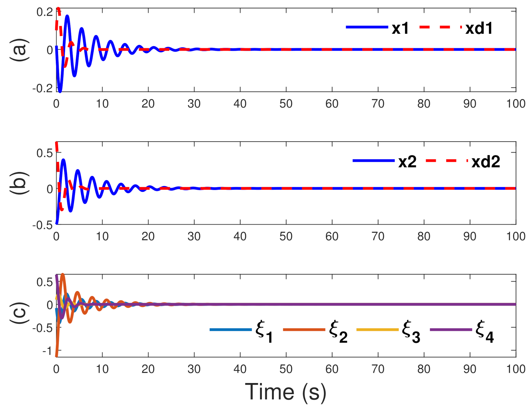
To make a comparison with DET via PE, during the neural network implementation process, a small probing noise is injected in u for the first 90 s. Figure 1 presents the evolution of the tracking system states and the augmented system states with DET via PE technique. Figure 2 presents the evolution of the tracking system states and the augmented system states with DET-based ER technique. From Figure 1 and Figure 2, it is obvious that the convergence of states and tracking trajectories via ER method is faster than the PE method. The optimal control $u_0$, the ISMC law $u_1$, the composite law u, and the sliding mode function S are shown in Figure 3 and Figure 4, for DET via PE technique and DET via ER technique, respectively. From Figure 3 and Figure 4, we can see that the convergence via ER method is faster than the PE method. The initial weights are selected randomly in the interval $[0,1]$. After a learning process, Figure 5 presents the convergence process of the critic NN weights ${\omega }_c$. The evolution of the event error $\left|\right|e_i{\left|\right|}^2$ and triggering threshold $\left|\right|e_T{\left|\right|}^2$ are shown in Figure 6. The interevent time of the control $u_0$ under under the four strategies is shown in Figure 7. Next, the characteristics of the different strategies are analyzed by comparison through Table 1, Table 2 and

Table 3. Trigger rates of different dets based on ER.

	Triggering Rate (%)	$\mathit{\lambda }$	0.01	0.1	0.5	1
$\mathit{\theta }$
0.1			24.90	25.10	25.45	25.65
0.5			22.10	22.90	25	25.80
1			17.10	20.80	25.25	26.60
3			1.75	3.6	26.30	27.50

.

First, Table 1 shows the data comparison for the four control strategies. As is well known, the number of triggering events is one of most important factors in evaluating the triggering mechanism. Furthermore, a smaller number of triggering events can reduce the communication burden and save resources. To implement this goal, it is needed to reduce the unnecessary update of the controller guaranteeing system performance. Based on this, a novel adaptive adjustment technique consisting of DET via ER technique is used. In addition, with the help of the simulation experiment platform and MATLAB data package, using respectively the technology in [39,40] and our technique in this paper, some experimental results are shown in Table 1. From Table 1, it is obvious that the DET via ER technique is the best, and which can better reduce the communication burden and save resources, since there are only 418 samples that occurred because of the larger average triggering interval time 0.2392 s. In particular, one may notice that the ER technique is also beneficial in reducing the number of event-triggering comparing with the PE technique in the framework of the same event-triggered conditions. Similarly, the DET is also beneficial in reducing the number of event-triggering comparing with ET in the framework of the same PE technique (ER technique). In addition, the minimal interval indicates Zeno-free behaviors. The minimal interval values of the four strategies are consistent with Figure 7. Moreover, according to Figure 7, we know that DET via ER technique can generate a biggest minimal interval comparing with other technique, so the effectiveness of the current technique designed in this paper is verified.

Next, we define another important factor to evaluate the control strategy, (called a triggering rate based on TT). The triggering rate is calculated by $\frac{{\mathrm{DET}}_{\mathrm{number}}}{{\mathrm{TT}}_{\mathrm{number}}}$. When $\theta =1$ and $\lambda =0.01$, Table 2 and Table 3 present that the rate of DET via PE and the rate of DET via ER are $23.75\%$ and $20.08\%$, respectively. Generally speaking, a small triggering rate is more favorable than a large triggering rate. To investigate the characteristics of the changes utilized to execute the triggering rule, some data of the triggering rates are shown in Table 2 and Table 3.The tables also show the effect of the parameters on the triggering rate generated by $\theta$ and $\lambda$ with DET via PE and ER respectively. To summary, a bigger $\theta$ value means a reduction of the number of events; in contrast, a bigger $\lambda$ value means an increase in the number of events.

Remark 4.

${\mathrm{ET}}_{\mathrm{PE}}$ is ET via PE technique, ${\mathrm{ET}}_{\mathrm{ER}}$ is ET via ER technique, ${\mathrm{DET}}_{\mathrm{PE}}$ is DET via PE technique, and ${\mathrm{DET}}_{\mathrm{ER}}$ is DET via ER technique.

6. Conclusions

In this article, a learning-based event-triggered optimal tracking control technique for nonlinear systems was developed via ADP. Matched uncertainties have been eliminated by the ISMC proposed in this paper. Unmatched uncertainties have been attenuated, utilizing projection matrix and an optimal controller. A critic NN via a novel dynamic event-triggered rule has been constructed to ensure the existence of the solution of the HJI equation and all errors have been proved UUB using the Lyapunov analysis method. Moreover, the simulation results revealed that our control algorithm is more favorable than traditional event-triggered control algorithms. Future work is to further explore this framework, e.g., in the presence of various delays or system constraints.

Remark 5.

(1) The pros: This study first provides codesign of dynamic event mechanism and experience replay technique-based weighted adaptive adjustment technique to guarantee the optimal approximation of the cost function $V^{*}$. In addition, this codesign technique not only speeds up the approximation speed of the cost function but also enlarges the average interval of internal events aiming to reduce the updating times of the controller and save the calculation burden and communication resources.

(2) The cons: In the proof Theorem 2, using the approximate the sign function $\mathrm{sgn}\left(S\right)\approx \tanh (S/\nu )$ where $\nu \ge 1$ that makes us to only obtain an approximation condition rather than a sufficient condition, namely, which weakens the effect of sliding-mode control. This issue should be investigated further.

References

- Isermann, R. Digital Control Systems; Springer Science & Business Media: Berlin/Heidelberg, Germany, 2013. [Google Scholar]
- Astrom, K.J.; Bernhardsson, B.M. Comparison of Riemann and Lebesque sampling for first order stochastic systems. In Proceedings of the 41st IEEE Conference on Decision and Control, Las Vegas, NV, USA, 10–13 December 2002; pp. 2011–2016. [Google Scholar]
- Tabuada, P. Event-triggered real-time scheduling of stabilizing control tasks. IEEE Trans. Autom. Control 2007, 52, 1680–1685. [Google Scholar] [CrossRef] [Green Version]
- Girard, A. Dynamic Triggering Mechanisms for Event-Triggered Control. IEEE Trans. Autom. Control 2015, 60, 1992–1997. [Google Scholar] [CrossRef] [Green Version]
- Ding, L.; Han, Q.L.; Ge, X.; Zhang, X.M. An overview of recent advances in event-triggered consensus of multi-agent systems. IEEE Trans. Cybern. 2018, 48, 1110–1123. [Google Scholar] [CrossRef] [PubMed] [Green Version]
- Peng, C.; Li, F. A survey on recent advances in event-triggered communication and control. Inf. Sci. 2018, 457, 113–125. [Google Scholar] [CrossRef]
- Zhang, X.M.; Han, Q.L.; Zhang, B.L. An overview and deep investigation on sampled-data-based event-triggered control and filtering for networked systems. IEEE Trans. Ind. Inform. 2016, 13, 4–16. [Google Scholar] [CrossRef]
- Pan, Y.; Yang, G.H. Event-triggered fault detection filter design for nonlinear networked systems. IEEE Trans. Syst. Man Cybern. Syst. 2008, 48, 1851–1862. [Google Scholar] [CrossRef]
- Ye, C.; Song, Y. Event-Triggered Prescribed Performance Control for a Class of Unknown Nonlinear Systems. IEEE Trans. Syst. Man Cybern. Syst. 2021, 51, 6576–6586. [Google Scholar]
- Ge, X.; Han, Q.; Zhang, X.M.; Ding, D. Dynamic event-triggered control and estimation: A survey. Int. J. Autom. Comput. 2021, 18, 857–886. [Google Scholar] [CrossRef]
- Ge, X.; Han, Q.L.; Ding, L.; Wang, Y.L.; Zhang, X.M. Dynamic event-triggered distributed coordination control and its applications: A survey of trends and techniques. IEEE Trans. Syst. Man Cybern. Syst. 2020, 50, 3112–3125. [Google Scholar] [CrossRef]
- Niu, Y.; Ho, D.W.C.; Lam, J. Robust integral sliding mode control for uncertain stochastic systems with time-varying delay. Automatica 2005, 41, 873–880. [Google Scholar] [CrossRef]
- Roy, S.; Baldi, S.; Fridman, L.M. Adaptive sliding mode control without a priori bounded uncertainty. Automatica 2020, 111, 1–6. [Google Scholar] [CrossRef]
- Roy, S.; Roy, S.B.; Lee, J.; Baldi, S. Overcoming the Underestimation and Overestimation Problems in Adaptive Sliding Mode Control. IEEE/ASME Trans. Mechatron. 2019, 24, 2031–2039. [Google Scholar] [CrossRef] [Green Version]
- Yu, W.; Wang, H.; Cheng, F.; Yu, X.; Wen, G. Second-Order Consensus in Multiagent Systems via Distributed Sliding Mode Control. IEEE Trans. Cybern. 2017, 47, 1872–1881. [Google Scholar] [CrossRef] [PubMed]
- Corradini, M.L.; Cristofaro, A. Nonsingular terminal sliding-mode control of nonlinear planar systems with global fixed-time stability guarantees. Automatica 2018, 95, 561–565. [Google Scholar] [CrossRef]
- Li, H.; Shi, P.; Yao, D. Adaptive sliding-mode control of Markov jump nonlinear systems with actuator faults. IEEE Trans. Autom. Control 2017, 64, 1933–1939. [Google Scholar] [CrossRef]
- Castan˜os, F.; Fridman, L. Analysis and Design of Integral Sliding Manifolds for Systems With Unmatched Perturbations. IEEE Trans. Autom. Control 2006, 51, 853–858. [Google Scholar] [CrossRef] [Green Version]
- Truc, L.N.; Vu, L.A.; Thoan, T.V.; Thanh, B.T.; Nguyen, T.L. Adaptive Sliding Mode Control Anticipating Proportional Degradation of Actuator Torque in Uncertain Serial Industrial Robots. Symmetry 2022, 14, 957. [Google Scholar] [CrossRef]
- Xu, L.; Xiong, W.; Zhou, M.; Chen, L. A Continuous Terminal Sliding-Mode Observer-Based Anomaly Detection Approach for Industrial Communication Networks. Symmetry 2022, 14, 124. [Google Scholar] [CrossRef]
- Yan, H.; Zhang, H.; Zhan, X.; Wang, Y.; Chen, S.; Yang, F. Event-Triggered Sliding Mode Control of Switched Neural Networks With Mode-Dependent Average Dwell Time. IEEE Trans. Syst. Man Cybern. Syst. 2021, 51, 1233–1243. [Google Scholar] [CrossRef]
- Zheng, B.C.; Yu, X.; Xue, Y. Quantized feedback sliding-mode control: An event-triggered approach. Automatica 2018, 91, 126–135. [Google Scholar] [CrossRef]
- Nair, R.R.; Behera, L.; Kumar, S. Event-triggered finite-time integral sliding mode controller for consensus-based formation of multi-robot systems with disturbances. IEEE Trans. Control Syst. Technol. 2019, 27, 39–47. [Google Scholar] [CrossRef]
- Zhou, K.; Doyle, J.C.; Glover, K. Robust and Optimal Control; Prentice-Hall: Englewood Cliffs, NJ, USA, 1996. [Google Scholar]
- Vincent, T.L. Nonlinear and Optimal Control Systems; Wiley: New York, NY, USA, 1997. [Google Scholar]
- Lewis, F.L.; Vrabie, D.; Syrmos, V.L. Optimal Control; Wiley: New York, NY, USA, 2012. [Google Scholar]
- Basar, T.; Bernard, P. H∞-Optimal Control and Related Minimax Design Problems; Birkhäuser: Boston, MA, USA, 1995. [Google Scholar]
- Vrabie, D.; Lewis, F. Neural network approach to continuous-time direct adaptive optimal control for partially unknown nonlinear systems. Neural Netw. 2009, 22, 237–246. [Google Scholar] [CrossRef] [PubMed]
- Bellman, R.E. Dynamic Programming; Princeton University Press: Princeton, NJ, USA, 1957. [Google Scholar]
- Wang, F.Y.; Zhang, H.; Liu, D. Adaptive dynamic programming: An introduction. IEEE Comput. Intell. Mag. 2009, 4, 39–47. [Google Scholar] [CrossRef]
- Michailidis, I.; Baldi, S.; Kosmatopoulos, E.B.; Ioannou, P.A. Adaptive Optimal Control for Large-Scale Nonlinear Systems. IEEE Trans. Autom. Control 2017, 62, 5567–5577. [Google Scholar] [CrossRef] [Green Version]
- Liu, D.; Xue, S.; Zhao, B.; Luo, B.; Wei, Q. Adaptive Dynamic Programming for Control: A Survey and Recent Advances. IEEE Trans. Syst. Man Cybern. Syst. 2021, 51, 142–160. [Google Scholar] [CrossRef]
- Fan, Q.Y.; Yang, G.H. Adaptive actor-critic design-based integral sliding-mode control for partially unknown nonlinear systems with input disturbances. IEEE Trans. Neural Netw. Learn. Syst. 2016, 27, 165–177. [Google Scholar] [CrossRef]
- Qu, Q.; Zhang, H.; Yu, R.; Liu, Y. Neural network-based H∞ sliding mode control for nonlinear systems with actuator faults and unmatched disturbances. Neurocomputing 2018, 275, 2009–2018. [Google Scholar] [CrossRef]
- Zhang, H.; Qu, Q.; Xia, G.; Cui, Y. Optimal guaranteed cost sliding mode control for constrained-input nonlinear systems with matched and unmatched disturbances. IEEE Trans. Neural Netw. Learn. Syst. 2018, 29, 2112–2126. [Google Scholar] [CrossRef]
- Vamvoudakis, K.G. Event-triggered optimal adaptive control algorithm for continuous-time nonlinear systems. IEEE/CAA J. Autom. Sin. 2014, 1, 282–293. [Google Scholar]
- Zhang, Q.; Zhao, D.; Zhu, Y. Event-triggered H∞ control for continuous-time nonlinear system via concurrent learning. IEEE Trans. Syst. Man Cybern. Syst. 2017, 47, 1071–1081. [Google Scholar] [CrossRef]
- Xue, S.; Luo, B.; Liu, D. Event-Triggered Adaptive Dynamic Programming for Unmatched Uncertain Nonlinear Continuous-Time Systems. IEEE Trans. Neural Netw. Learn. Syst. 2020, 99, 1–13. [Google Scholar] [CrossRef] [PubMed]
- Yang, D.S.; Li, T.; Xie, X.P.; Zhang, H.G.; Liu, D.R.; Li, Y.H. Event-Triggered Integral Sliding-Mode Control for Nonlinear Constrained-Input Systems With Disturbances via Adaptive Dynamic Programming. IEEE Trans. Syst. Man Cybern. Syst. 2020, 50, 2168–2216. [Google Scholar] [CrossRef]
- Zhang, H.G.; Liang, Y.; Su, H.; Liu, C. Event-Driven Guaranteed Cost Control Design for Nonlinear Systems with Actuator Faults via Reinforcement Learning Algorithm. IEEE Trans. Syst. Man Cybern. Syst. 2020, 50, 4135–4150. [Google Scholar] [CrossRef]
- Van, M.; Do, X.P. Optimal adaptive neural PI full-order sliding mode control for robust fault tolerant control of uncertain nonlinear system. Eur. J. Control. 2020, 54, 22–32. [Google Scholar] [CrossRef]
Figure 1.
PE technique: (a,b) resulted trajectory compared with the desired trajectory with DET; (c) state trajectory.
Figure 2.
ER technique: (a,b) resulted trajectory compared with the desired trajectory with DET; (c) state trajectory of augmented systems.
Figure 3.
PE technique: (a) evolution of RL-based control law ; (b) evolution of SMC input ; (c) evolution of composite control law u; (d) evolution of sliding mode surface S.
Figure 4.
ER technique: (a) evolution of RL-based control law ; (b) evolution of SMC input ; (c) evolution of composite control law u; (d) evolution of sliding mode surface S.
Figure 5.
Weight curves of system states during learning stage.
Figure 6.
Trigger threshold and event error during learning stage.
Figure 7.
Inter-event time of four strategies during learning stage.