Optimization for an Indoor 6G Simultaneous Wireless Information and Power Transfer System

Abstract

Antenna beamforming for Simultaneous Wireless Information and Power Transfer (SWIPT) and Wireless Power Transfer (WPT) in an indoor 6G communication system is presented in this paper. The objective function is to maximize the total harvesting power for the SWIPT and WPT nodes with the constraints of the bit error rate and minimum harvesting power. In the study, the power-splitting ratio between harvesting power and decoding information can be adjusted for the SWIPT node. Due to the non-convex problem, we use Self-Adaptive Dynamic Differential Evolution (SADDE) to optimize the designed multi-objective function. We use a symmetric antenna array to study three situations of distance—closer, farther, and similar—between the transmitting antenna and the individual SWIPT and WPT nodes in this paper. Experimental results show that the overall harvesting efficiency is improved, especially in the case of SWIPT nodes closer to the transmitter. The total harvesting power can be improved by 86.7% in the total short-distance case, and by 7.87% in the total long-distance case.

1. Introduction

The 6G science and technology has developed very rapidly in recent years in order to improve the strength of transmitted and received signals, as well as system performance gain. Therefore, symmetric antenna arrays are widely used in communication, radar, and other systems. The focus of 6G communication is on four application areas: solving social problems, connecting people and things, building a broader communication environment, and achieving the complex integration of the virtual and the real [1,2,3,4]. The transmission capacity of 6G is probably 100 times higher than that of 5G, while the network latency is also reduced from milliseconds (1 ms) to microseconds (100 µs). The main purpose is to develop the internet. Power efficiency, spectral efficiency, air delay, connection density, reliability, peak data rate, and user experience data rate are far better than those of 5G mobile communication systems, which have been officially rolled out all over the world [5,6,7]. As 6G communication systems are being actively developed, in order to meet the goal of high-speed communication, the US Federal Communications Commission (FCC) suggests that the frequency band used for 6G should be 95 GHz to 3 THz. As 6G has higher speed, lower latency, and a wider connection range than 5G, more high-frequency resources such as millimeter and terahertz waves can be implemented with artificial intelligence technology to create more connections.

Energy-constrained and energy-consumptive are typical wireless device problems in the Internet of Things (IoT), although the wireless device can solve them by changing batteries [8,9]. However, it requires high operational costs, and is not feasible in some scenarios. WPT and SWIPT can solve this problem by replenishing energy from the ambient environment constantly. Moreover, the SWIPT can provide energy and transfer data at the same time. For some applications, the sensor can use the relay wireless signal or the base station wireless signal to harvest power when it has information transaction requirements. In the past, some studies on low-power IoT have used UAVs to improve the SWIPT/WPT charging efficiency and extend the transmission path of the base station [10]. There are also studies on the coverage and performance improvement of systems using SWIPT/WPT relays [11].

Some researchers have used deep learning methods to adjust the antenna for the SWIPT system [12,13]. SWIPT cooperative spectrum sharing for 6G-enabled cognitive IoT networks was proposed in [14]. SWIPT cooperative relays were discussed in [11]. Simultaneous WPT with IoT toward 6G has been presented in [15]. For THz beamforming in 6G communication systems, Wang used a reconfigurable intelligible surface for beaming [16]. Huang applied deep reinforcement learning to adjust a reconfigurable intelligent surface to improve the beaming technology [17]. Guo employed circuit multiple beaming networks to reduce the cost and power consumption [18]. Cataka proposed a mitigation method for adversarial attacks against 6G machine learning models for millimeter-wave beam prediction using adversarial training. The results show that the mean square errors of the defended model under attack are very close to those of the undefended model without attack [19].

Some studies on beamforming technology for SWIPT and WPT have been published in recent years [20,21,22,23,24]. The topologies for splitting-based SWIPT are investigated in [25,26,27]. Time-splitting, power-splitting, and frequency-splitting are the most popular ways to achieve SWIPT. In the power-splitting technique, a power-divided component is utilized to divide the received signal into two streams with a designed power ratio. The major merit is that the signal is used for both functions in the same time slot. For the evolution algorithm, Differential Evolution (DA) and SADDE have been used in the antenna beamforming design, as in [17,28]. The objective function used in this paper is the weighted sum of the individual objective functions, such as the antenna pattern, antenna sidelock, and scattering s-parameters. None of the BER is considered in these cases.

A lot of low-power sensors for 6G SWIPT/WPT IoT are placed in modern communication systems. SWIPT has an advantage compared with the conventional time-division multiplexing mechanism, where the transmissions of power and information are separate. In addition, past SWIPT power-splitting has used fixed splitting coefficients, but in fact, this may lead to excessive waste of transmission energy. Thus, if we can control the adjustment of the splitting coefficients dynamically, the harvest power efficiency can be improved a lot. Our proposed system can switch beams according to the sensors in the environment. As a result, overall high performance can be achieved.

Our novelty is to present beamforming technique optimization for SWIPT and WPT in 6G terahertz broadband communication systems. The beamforming technique is used to adjust the phase of the transmitter to find the maximum power harvesting efficiency under the constraint of the preset lowest bit error rate and lowest harvesting power. The bit error rate of the broadband signal is affected by the multipath and the power level at the same time, as the bit error rate is a nonlinear function and, thus, one cannot find the best solution by the differential method. The evolution algorithms are used to optimize the different requirements at the same time by the designed multi-objective function. The ray-tracing method is used to simulate the environment. Then, SADDE is used to optimize the synthetic field pattern of the antenna array to improve the system performance.

The structure of this article is listed as follows: Section 2 introduces the system model and the deployment of the antenna array. In Section 3, the evolution algorithm and objective function are presented. Numerical results are given in Section 4, where we compare the SWIPT and WPT using SADDE. The final section summarizes the contributions of this paper.

2. System Model

In the channel model, the ray-tracing method is used to calculate the loss and frequency response of 6G terahertz communication. The frequency response is denoted as follows:

$$H\left(f\right)={{\displaystyle \sum }}_{i=1}^N{\alpha }_i\left(f\right)e^{j\phi \left(f\right)}$$

(1)

where N is the total number of paths, f is the frequency, i is the path index of the ray, ${\alpha }_i$ is the i-th amplitude comprising the phase and intensity information, and $\phi$ is the phase shift delay. The time-domain impulse response of the equivalent baseband can be obtained by using the inverse Fourier transform.

$$h\left(t\right)={{\displaystyle \int }}_{-\infty }^{\infty }H\left(f\right)e^{j2\pi ft}df$$

(2)

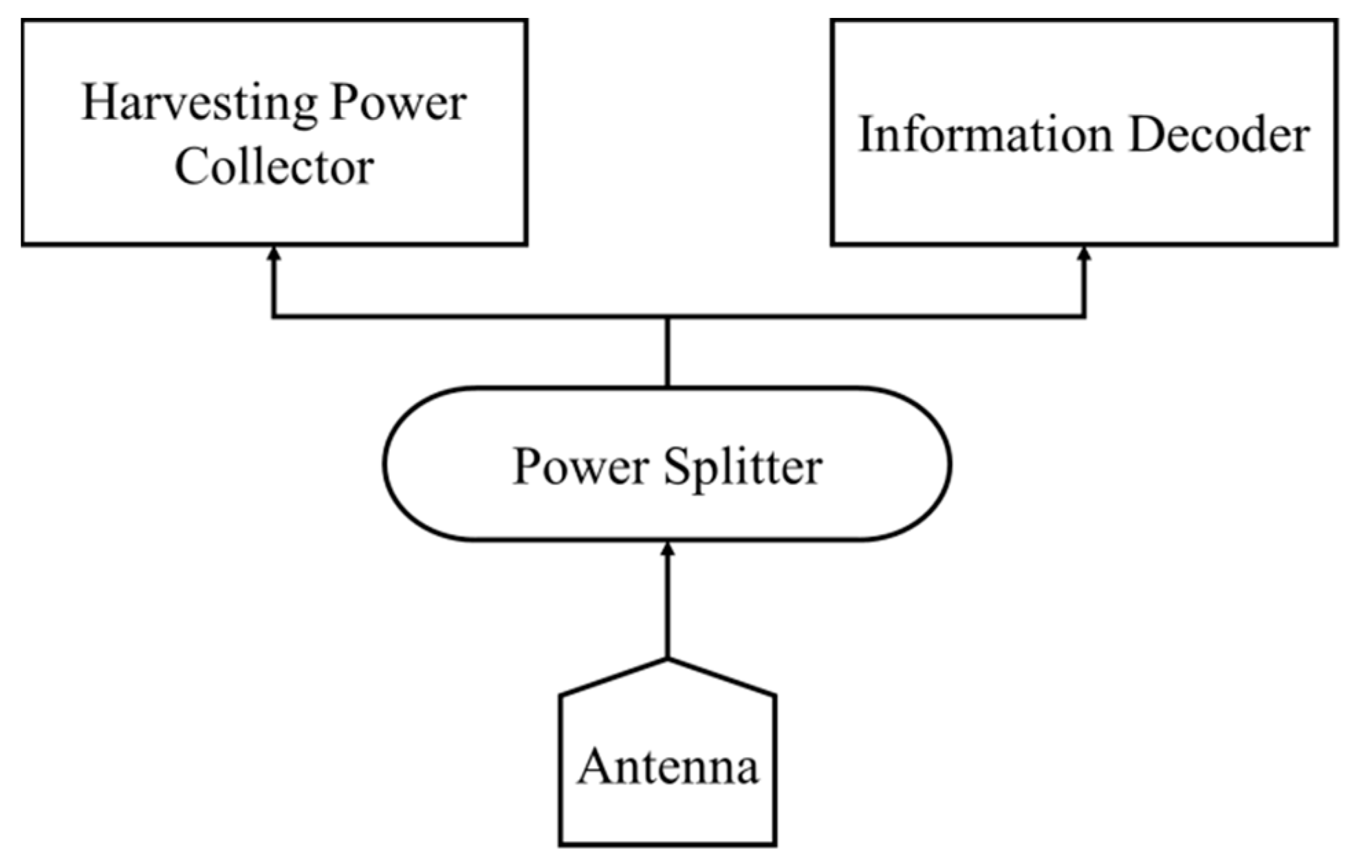
Figure 1 shows the SWIPT splitter structure. For simulation’s sake, the split rate of the power divider is set to $\alpha$ for the power harvester. The harvesting power collector and the information decoder are arranged in front of the power distributor.

The wireless harvesting power is modeled as the received energy per bit:

$$HP=\alpha \eta {{\displaystyle \int }}_{-\infty }^{\infty }h{\left(t\right)}^{2}dt$$

(3)

where $\eta$ is the portion of RF signal used for power acquisition, and $\alpha$ is the energy split ratio. The information decoder for BER is used to study the inter-symbol interference in our SWIPT system. Its calculation formula is as follows [29,30]:

$$BER={\sum }_{n=1}^{2^N}P\left({\stackrel{\rightharpoonup }{d}}_n\right)·\frac{1}{2}erfc[\frac{V_n}{\sqrt{2}\sigma }·(d_N)]$$

(4)

where $erfc\left(x\right)=\frac{2}{\sqrt{\mathsf{\pi }}}{\int }_x^{\infty }{e}^{-y^2}dy$ is the complementary error function, and V is the received signal after demodulation. $\left\{{\stackrel{\rightharpoonup }{d}}_n\right\}=\left\{d_1,d_2,\dots d_N\right\}$ is the binary sequence, and N is the number of bits.

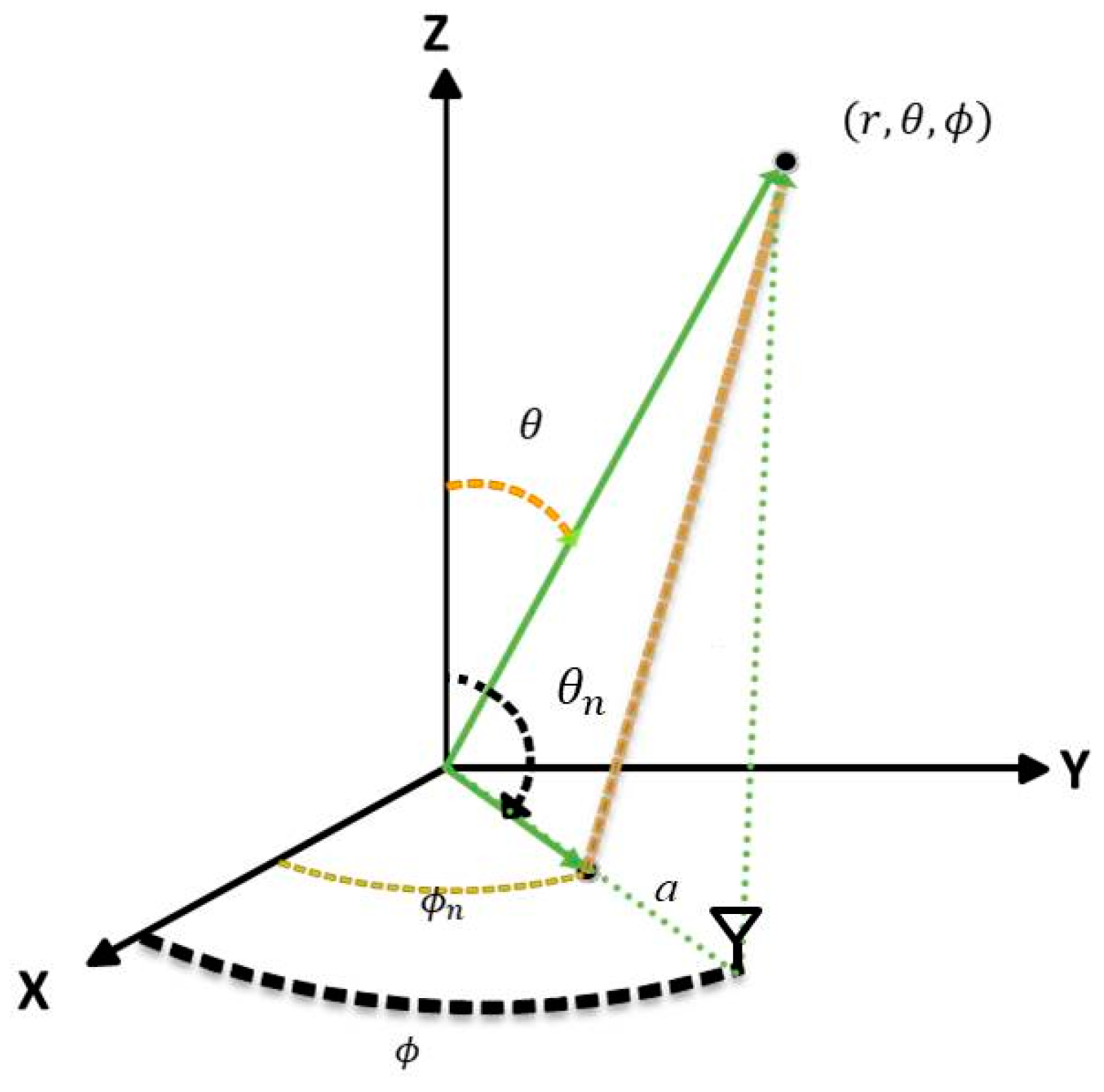
The array equivalent mode is calculated by the array factor, and the coordinate relationship is shown in Figure 2.

According to Figure 2, we can express the array factor as follows:

$$AF\left(\theta ,\varphi ,f\right)={\displaystyle \sum }_{n=1}^M{W}_n{e}^{jka\left[sin\theta sin{\theta }_{n}cos\left(\varphi -{\varphi }_n\right)+cos{\theta }_{n}cos\theta \right]}$$

(5)

where M is the total number of antennas in the array, a is the distance between the antenna location and the origin, ${\theta }_n$ and ${\varphi }_n$ are the polar angle and azimuthal angle of the transmitter, respectively, the azimuthal angle $\varphi$ and $\mathrm{polar}\mathrm{angle}\theta$ are the spherical coordinates system, and k is equal to $2\pi$ divided by the wavelength. The adjustment for phase delay and antenna power can be expressed as follows:

$$W_m=I_m{e}^{j{D}_m\left(f\right)}$$

(6)

where $D_m\left(f\right)$ is the excitation current and $I_m$ is the phase delay. The relationship between feed length and $D_m\left(f\right)$ can be expressed as follows:

$$D_m\left(f\right)=-\frac{2\pi f}{c}\sqrt{{\epsilon }_r}·{\ell }_n$$

(7)

where ${\epsilon }_r$ is the relative dielectric constant of the feeder and ${\ell }_n$ is the feeder length of the transmission line, which can be used to adjust the phase delay; c is the light speed.

3. Evolution Algorithm

Dynamic Differential Evolution (DDE) is further developed into Self-Adaptive Dynamic Differential Evolution (SADDE). The SADDE algorithm adds a dynamic mechanism to the adjustment factor during the DDE search [31]. The flowchart of the SADDE algorithm is shown in Figure 3.

First, the population parameters are randomly initialized. The objective function of the antenna array is calculated by using M-dimensional adjustment parameters. The position of the particle is adjusted according to the parameters. From the calculation of the objective function, the optimal particle is updated accordingly. The test vector then adjusts the control vector in the next calculation, and decides whether to use the crossover mechanism based on a preset probability. After crossover, the new particle is compared to the previous target value, and the position of the globally optimal particle is renewed.

The detailed steps are as follows:

Step 1

First, the population parameters are initialized randomly. During the initialization process, the population is initialized as a $D_s$-dimensional vector, where $D_s$ denotes the number of parameters.

Step 2

The $D_s$-dimensional adjustment parameters are used to calculate the objective function for any antenna array. The objective functions for $L_p$ particles are then evaluated, where $L_p$ denotes the population size. Based on the calculated value from our objective functions, the best particle is updated accordingly.

Step 3

In adjusting the control vectors ${\mathsf{\nu }}_i^{g+1}$ and ${\mathsf{\xi }}_i^{g+1}$ of the next iteration, the mutation process is composed of arithmetic combination, by adjusting the test vector ${\mathsf{\Omega }}_i^{g+1}$, which is generated from the parent parameter vector ${\mathsf{\Lambda }}_i^g$ by the following equation:

$$\begin{gathered} {\left({\mathsf{\Omega }}_i^{g+1}\right)}_j={\left({\mathsf{\Lambda }}_i^g\right)}_j+{\mathsf{\nu }}_i^g·\left[{\left({\mathsf{\Lambda }}_{best}^g\right)}_j-{\left({\mathsf{\Lambda }}_i^g\right)}_j\right]+{\mathsf{\xi }}_i^g·\left[{\left({\mathsf{\Lambda }}_m^g\right)}_j-{\left({\mathsf{\Lambda }}_n^g\right)}_j\right] \\ m,n\in \left[1,L_p\right],m\ne n \end{gathered}$$

(8)

$${\mathsf{\nu }}_i^{g+1}=\{\begin{array}{cc}{\mathsf{\nu }}_l+ran{d}_a\times {\mathsf{\nu }}_u,& ifran{d}_b<0.1\\ {\mathsf{\nu }}_i^g,& otherwise\end{array}$$

(9)

$${\mathsf{\xi }}_i^{g+1}=\{\begin{array}{cc}{\mathsf{\xi }}_l+ran{d}_c\times {\mathsf{\xi }}_u,& ifran{d}_d<0.1\\ {\xi }_i^g,& otherwise\end{array}$$

(10)

where ${\mathsf{\nu }}_i$ and ${\mathsf{\nu }}_u$ are the lower and upper limits of $\mathsf{\nu }$, respectively. ${\mathsf{\xi }}_l$ and ${\mathsf{\xi }}_u$ are the lower and upper limits of $\mathsf{\xi }$, respectively. $ran{d}_a$, $ran{d}_b$, $ran{d}_c$, and $ran{d}_d$ are uniformly distributed random numbers from 0 to 1.

Step 4

In the crossover mechanism, crossover is determined according to the probability of $C{o}_i$, and the equation is as follows:

$${\left({\mathsf{\Gamma }}_i^{g+1}\right)}_j=\{\begin{array}{cc}{\left({\mathsf{\Omega }}_i^{g+1}\right)}_j,& \zeta \left(j\right)<C{o}_i^g\\ {\left({\mathsf{\Lambda }}_i^g\right)}_j,& \zeta \left(j\right)\ge C{o}_i^g\end{array}$$

(11)

$$C{o}_i^{g+1}=\{\begin{array}{cc}ran{d}_e,& ifran{d}_f<0.1\\ C{o}_i^g,& otherwise\end{array}$$

(12)

where $\zeta \left(j\right)$, $ran{d}_e$, and $ran{d}_f$ are the random numbers.

Step 5

The vector with the smaller objective function is used to update the position of the global best particle.

Step 6

Finally, we decide to execute or stop the algorithm according to the iteration number and the convergent condition.

In order to meet the different requirements concurrently, multi-objective functions are considered in the algorithm. The goal is to find the maximum total harvesting power with constraints. The constraints include the bit error rate as well as the minimum harvesting power for the SWIPT and WPT nodes. The total harvesting power is expressed by the following equation:

$$H{P}_T={\displaystyle \sum }_{m=1}^{M_R}H{P}_m$$

(13)

where $M_R$ is the total number of receivers in the environment.

The $BER$ constraint is defined as ${10}^{-5}$, so that $BE{R}_W$ is expressed as follows:

$$BE{R}_W=\{\begin{array}{c}\frac{{10}^{-5}}{BER},BER>{10}^{-5}\\ 1,BER<{10}^{-5}\end{array}$$

(14)

The minimum harvesting power for SWIPT is set at $5\times {10}^{-8}$ as the second constraint. $H{P}_{SWIPT}$ is defined as follows:

$$H{P}_{SWIPT}=\{\begin{array}{c}\frac{H{P}_1}{5\times {10}^{-8}},H{P}_1<5\times {10}^{-8}\\ 1,H{P}_1>5\times {10}^{-8}\end{array}$$

(15)

The minimum harvesting power for WPT is set at $1.5\times {10}^{-7}$ as the third constraint. $H{P}_{WPT}$ is defined as follows:

$$H{P}_{WPT}=\{\begin{array}{c}\frac{H{P}_2}{1.5\times {10}^{-7}},H{P}_2<1.5\times {10}^{-7}\\ 1,H{P}_2>1.5\times {10}^{-7}\end{array}$$

(16)

The objective function is assumed to be:

$$BE{R}_W\times H{P}_{SWIPT}\times H{P}_{WPT}\times H{P}_T$$

(17)

From Equation (17), when the BER is reduced to ${10}^{-5}$, along with the minimum harvesting power constraint being satisfied, the total harvesting power can be maximized as much as possible.

4. Numerical Results

Terahertz waves were deployed as the indoor communication system in our research. The frequency was set from 99 GHz to 109 GHz in a sixth-generation communication system with 48 antennas. The SWIPT node was Rx1. The power collection node was Rx2. Figure 4 shows the floor plan of the actual simulation environment. The Tx antenna was located at the center of the room (5, 5, 1 m). In order to investigate the performance against the location factor, three different distance scenarios were arranged between the receiving antennas Rx1 and Rx2 and the Tx antenna. The first scenario placed Rx1 farther away from Tx than Rx2. Here, Rx1 (9, 7, 1 m) and Rx2 (2, 6, 1 m) corresponded to the longer total distance (i.e., Rx1 to Tx plus Rx2 to Tx), while Rx1 (7, 2, 1 m) and Rx2 (3, 6, 1 m) corresponded to the shorter total distance. In the second scenario, Rx1 was placed closer to Tx than Rx2. Rx1 (5, 8, 1 m) and Rx2 (2, 2, 1 m) corresponded to the longer total distance, while Rx1 (6, 6, 1 m) and Rx2 (2, 5, 1 m) corresponded to the shorter total distance. In the third scenario, the distance of Rx1 and Rx2 from Tx was less than 1 m. Rx1 (9, 8, 1 m) and Rx2 (3, 1, 1 m) corresponded to the longer total distance, while Rx1 (7, 8, 1 m) and Rx2 (2, 7, 1 m) corresponded to the shorter total distance.

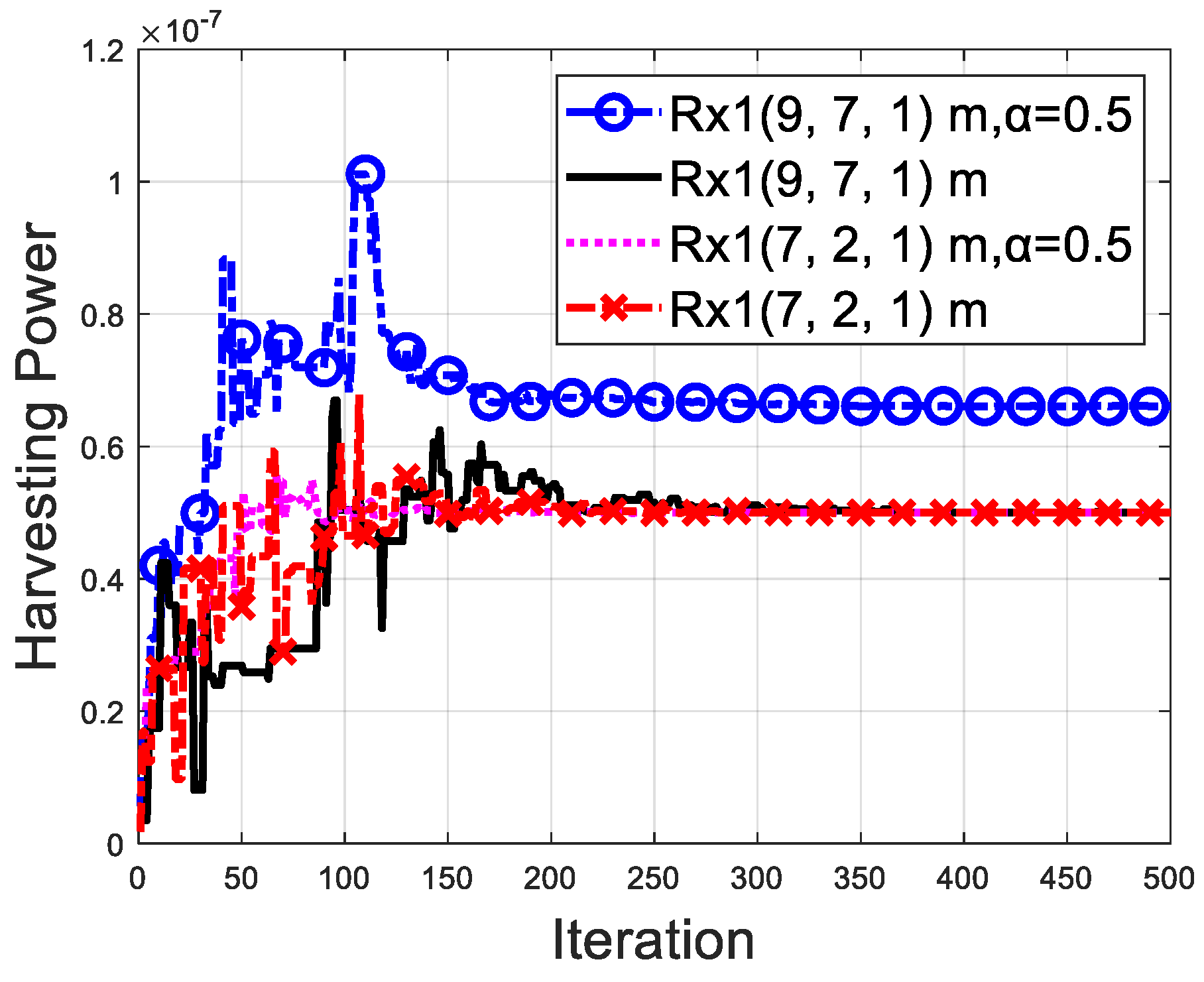
In the first scenario, Rx1 was farther away from Tx than Rx2. Figure 5 and Figure 6 show the SWIPT and WPT harvesting power, respectively, with and without α adjustment, where $\alpha =0.5$ (power allocation ratio) is preset for the case without optimization adjustment. It can be seen that the convergence was reached after 200 iterations. The harvesting power for the WTP node was slightly increased with the power-splitting adjustment.

Table 1. Harvesting power ratios for Rx1 (9, 7, 1) and Rx2 (2, 6, 1).

	BER	Harvesting Power Ratio	Harvesting Power Ratio Improvement	α
Rx1	O	$6.61\times {10}^{-8}$	7.15%	0.5
Rx2		$2.54\times {10}^{-7}$
Rx1 (α)	O	$5.00\times {10}^{-8}$		0.44
Rx2 (α)		$2.93\times {10}^{-7}$

shows the harvesting power ratio for the first group Rx1 (9, 7, 1 m) and Rx2 (2, 6, 1 m), in which the harvesting power ratio was increased by about 7.15% by $\alpha$ adjustment. As long as the BER and minimum harvesting power requirement for Rx1 are met, the excess power can be efficiently allocated to Rx2 during the field adjustment process. Under this circumstance, the total power for Rx1 plus Rx2 is increased.

Table 2. Harvesting power ratios for Rx1 (7, 2, 1) and Rx2 (3, 6, 1).

	BER	Harvesting Power Ratio	Harvesting Power Ratio Improvement	α
Rx1	O	$5.00\times {10}^{-8}$	2.6%	0.5
Rx2		$4.88\times {10}^{-7}$
Rx1 (α)	O	$5.00\times {10}^{-8}$		0.53
Rx2 (α)		$5.02\times {10}^{-7}$

shows the harvesting power for the second group, Rx1 (7, 2, 1 m) and Rx2 (3, 6, 1 m). We can see that the harvesting power for Rx1 without (α = 0.5) and with power-splitting adjustment (α = 0.53) is the same. This is because the antenna pattern is changed when α is being adjusted. In other words, the antenna gain towards Rx1 is decreased while the power-splitting ratio is increased. Moreover, when the antenna gain towards Rx2 is increased, the harvesting power for Rx2 is also increased. In the end, the total harvesting power of Rx1 plus Rx2 is increased by 2.6% compared with that of α = 0.5. The random search for the first generation is used in the SADDE algorithm. The different random seed affects the convergence of our problem. However, if we use enough iterations, we can obtain an accurate result.

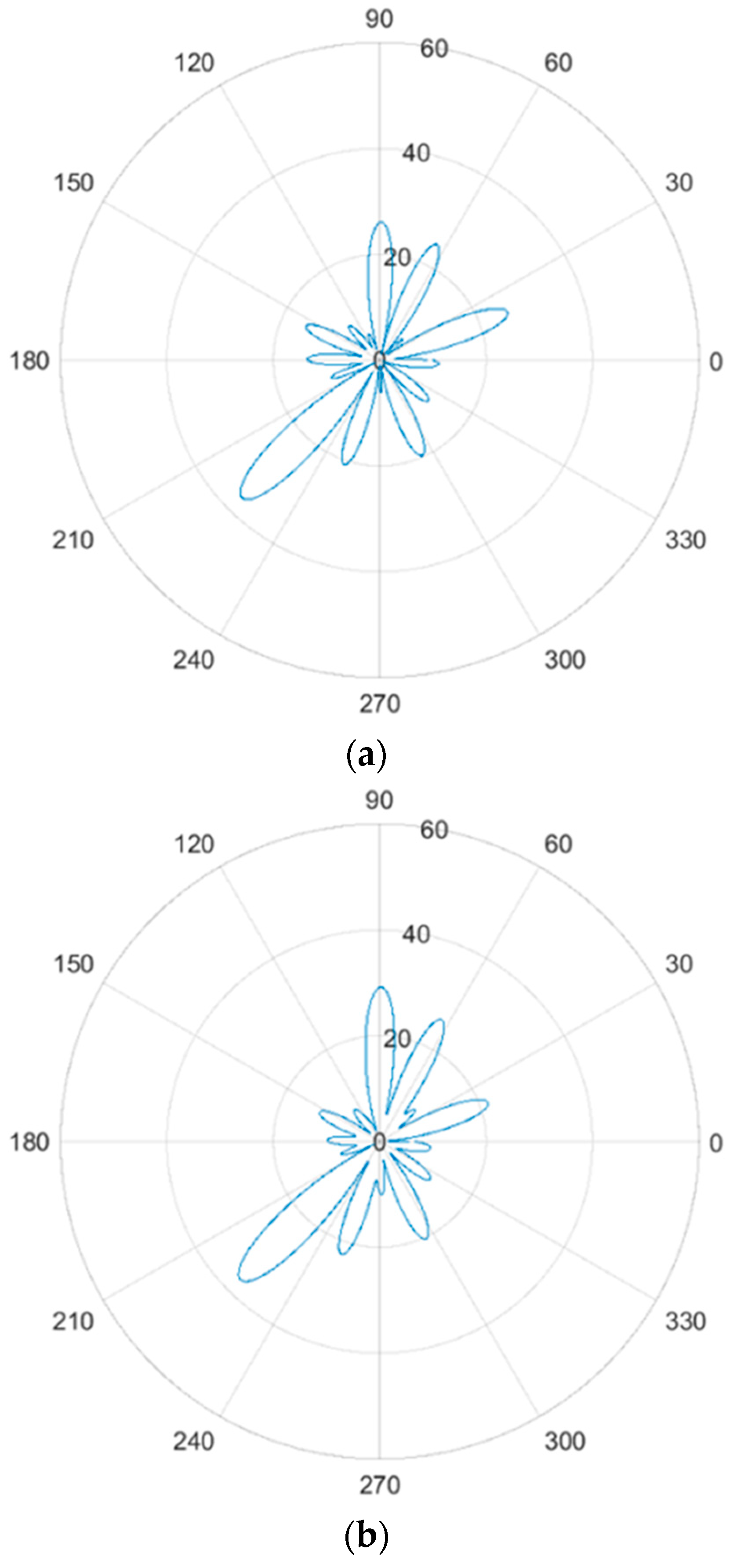
In the second scenario, Rx2 is closer to Tx, and Rx1 is farther from Tx. Figure 7 and Figure 8 show the SWIPT and WPT harvesting power, respectively, with and without α adjustment, where α = 0.5 (power allocation ratio) is preset for the case without optimization adjustment. Simulations showed that the harvesting power was convergent at about 250 iterations. The harvesting power for the SWIPT node was increased by adjusting the power-splitting ratio.

Table 3. Harvesting power ratios for Rx1 (5, 8, 1) and Rx2 (2, 2, 1).

	BER	Harvesting Power Ratio	Harvesting Power Ratio Improvement	α
Rx1	O	$8.53\times {10}^{-8}$	7.87%	0.5
Rx2		$1.59\times {10}^{-7}$
Rx1 (α)	O	$1.13\times {10}^{-7}$		0.59
Rx2 (α)		$1.50\times {10}^{-7}$

shows the harvesting power ratio for the first group Rx1 (5, 8, 1) and Rx2 (2, 2, 1). It can be seen that the harvesting power ratio was increased about 7.87% due to α adjustment. As long as the minimum power harvesting requirement for Rx2 is met, the harvesting power can be efficiently allocated to Rx1 through α adjustment. Consequently, the total power for Rx1 plus Rx2 can be obtained.

Table 4. Harvesting power ratios for Rx1 (6, 6, 1) and Rx2 (2, 5, 1).

	BER	Harvesting Power Ratio	Harvesting Power Ratio Improvement	α
Rx1	O	$5.74\times {10}^{-7}$	86.7%	0.5
Rx2		$1.50\times {10}^{-7}$
Rx1 (α)	O	$1.20\times {10}^{-6}$		0.95
Rx2 (α)		$1.50\times {10}^{-7}$

shows the harvesting power for the second group of Rx1 (6, 6, 1 m) and Rx2 (2, 5, 1 m). In this case, the harvesting power ratio for Rx1 was increased due to the large power-splitting factor (α = 0.95). Again, the harvesting power ratio for Rx2 without (0.5α) and with (0.95α) power-splitting adjustment was the same. Eventually, the total harvesting power for Rx1 plus Rx2 increased by 86.7% compared with that of α = 0.5. Figure 9 shows the radiation pattern from the transmitter to Rx1 (6, 6, 1 m) and Rx2 (2, 5, 1 m). The diagrams illustrate that both beams point correctly towards Rx1 (6, 6, 1 m) and Rx2 (2, 5, 1 m). However, the gain for the case with power-splitting adjustment is slightly greater than that without power-splitting adjustment.

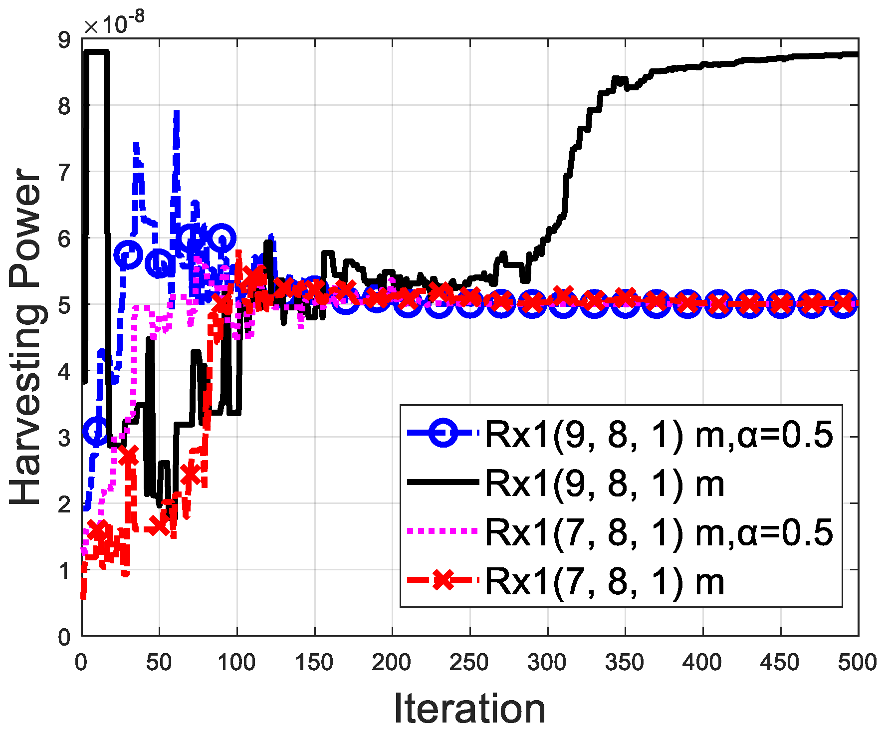
In the third scenario, the distance of Rx1 and Rx2 from Tx was less than 1 m. Figure 10 and Figure 11 show the SWIPT and WPT harvesting power, respectively, with and without α adjustment, where α = 0.5 (the power allocation ratio) is preset for the case without optimization adjustment. Convergence was reached after 350 iterations.

Table 5. Harvesting power ratios for Rx1 (9, 8, 1) and Rx2 (3, 1, 1).

	BER	Harvesting Power Ratio	Harvesting Power Ratio Improvement	α
Rx1	O	$5.00\times {10}^{-8}$	0.13%	0.5
Rx2		$1.87\times {10}^{-7}$
Rx1 (α)	O	$8.76\times {10}^{-8}$		0.63
Rx2 (α)		$1.50\times {10}^{-7}$

shows the harvesting power ratio for the first group Rx1 (9, 8, 1 m) and Rx2 (3, 1, 1 m). It can seen that the harvesting power ratio was increased by about 0.13% due to α adjustment. As long as the minimum power harvesting requirement for Rx2 is achieved, the excess power can be efficiently allocated to Rx1 through α adjustment of the antenna gain during the field adjustment process. Ultimately, the total power for Rx1 plus Rx2 is only slightly increased.

Table 6. Harvesting power ratios for Rx1 (7, 8, 1) and Rx2 (2, 7, 1).

	BER	Harvesting Power Ratio	Harvesting Power Ratio Improvement	α
Rx1	O	$5.00\times {10}^{-8}$	0.52%	0.5
Rx2		$1.80\times {10}^{-7}$
Rx1 (α)	O	$5.02\times {10}^{-8}$		0.55
Rx2 (α)		$1.81\times {10}^{-7}$

shows the harvesting power ratio for the second group, Rx1 (7, 8, 1 m) and Rx2 (2, 7, 1 m). It can be seen that the harvesting power ratio was increased by about 0.52% via α adjustment. Note that the power collected by Rx1 before (α = 0.5) and after (α = 0.55) the adjustment was similar. This is due to the fact that the antenna gains for Rx1 and Rx2 can be adjusted during the α optimization process. Subsequently, by reducing the antenna gain of Rx1, the algorithm can still meet the BER and minimum power harvesting requirement constraints by increasing α, and the excess power can then be allocated to Rx2. For this case, the total power of Rx1 plus Rx2 is increased by 0.52% compared with that of α = 0.5.

5. Conclusions

In this paper, the millimeter-wave frequency band of the future sixth-generation mobile communication system is analyzed and presented. The impact of the actual environment on the millimeter wave band is taken into account by the ray-bouncing tracking method, and the frequency of 99–109 GHz is used for optimization analysis. The distance between the transmitter and the SWIPT as well as WPT nodes is considered for our study. SWIPT nodes need to consider the communication quality and the harvesting power simultaneously. On the other hand, WPT nodes only need to consider the harvesting power. To satisfy the bit error rate constraint—the basic power requirements for SWIPT nodes and WPT nodes—a special objective function is employed, and it is ultimately solved the by Self-Adaptive Dynamic Differential Evolution method. In summary, SWIPT can achieve basic communication quality and, in the meantime, can maintain the minimum harvesting power requirement by applying the multi-objective function algorithm. In the first scenario, the improvement in efficiency by power-splitting adjustment is affected by the total distance. Since the WPT can easily meet the constraint via SADDE with the designed objective function at a closer total distance, the power-splitting improvement is only 2.6%, but the improvement is 7.15% better at a greater total distance. Moreover, the second scenario’s results show that when the WPT node is closer to the transmitter and the SWIPT node is farther from transmitter, the total harvesting power can be improved by 7.87% in the total long-distance case. However, the third scenario’s results show that when the SWIPT node is placed closer to Tx, the total harvesting power can be improved by 86.7%. This is due to the fact that when the total distance is lower than that in the second scenario, the constraints are easy to achieve, and the power-splitting adjustment has more flexibility to improve the total efficiency. Finally, the system efficiency is improved overall, while the targeted bit error rate constraints can be met in all cases as well. However, our algorithm is very time-consuming. We intend to modify and speed up the algorithm in the future.

References

- Lee, Y.L.; Qin, D.; Wang, L.-C.; Sim, G.H. 6G Massive Radio Access Networks: Key Applications, Requirements and Challenges. IIEEE Open J. Veh. Technol. 2021, 2, 54–66. [Google Scholar] [CrossRef]
- Tataria, H.; Shafi, M.; Molisch, A.F.; Dohler, M.; Sjöland, H.; Tufvesson, F. 6G Wireless Systems: Vision, Requirements, Challenges, Insights, and Opportunities. Proc. IEEE 2021, 109, 1166–1199. [Google Scholar] [CrossRef]
- De Lima, C.; Belot, D.; Berkvens, R.; Bourdoux, A.; Dardari, D.; Guillaud, M.; Isomursu, M.; Lohan, E.-S.; Miao, Y.; Wymeersch, H.; et al. Convergent Communication, Sensing and Localization in 6G Systems: An Overview of Technologies, Opportunities and Challenges. IEEE Access 2021, 9, 26902–26925. [Google Scholar] [CrossRef]
- Verma, S.; Kaur, S.; Khan, M.A.; Sehdev, P.S. Toward Green Communication in 6G-Enabled Massive Internet of Things. IEEE Internet Things J. 2021, 8, 5408–5415. [Google Scholar] [CrossRef]
- Ansari, R.I.; Chrysostomou, C.; Hassan, S.A.; Guizani, M.; Mumtaz, S.; Rodriguez, J.; Rodrigues, J.J. 5G D2D Networks: Techniques, Challenges, and Future Prospects. IEEE Syst. J. 2018, 12, 3970–3984. [Google Scholar] [CrossRef]
- Shafique, K.; Khawaja, B.A.; Sabir, F.; Qazi, S.; Mustaqim, M. Internet of Things (IoT) for Next-Generation Smart Systems: A Review of Current Challenges, Future Trends and Prospects for Emerging 5G-IoT Scenarios. IEEE Access 2020, 8, 23022–23040. [Google Scholar] [CrossRef]
- Zhou, B.; Liu, A.; Lau, V. Successive Localization and Beamforming in 5G mmWave MIMO Communication Systems. IEEE Trans. Signal Process. 2019, 67, 1620–1635. [Google Scholar] [CrossRef]
- Huang, J.; Xing, C.-C.; Wang, C. Simultaneous Wireless Information and Power Transfer: Technologies, Applications, and Research Challenges. IEEE Commun. Mag. 2017, 55, 26–32. [Google Scholar] [CrossRef]
- Perera, T.D.P.; Jayakody, D.N.K.; Sharma, S.K.; Chatzinotas, S.; Li, J. Simultaneous Wireless Information and Power Transfer (SWIPT): Recent Advances and Future Challenges. IEEE Commun. Surv. Tutor. 2017, 20, 264–302. [Google Scholar] [CrossRef] [Green Version]
- Wang, X.; Gursoy, M.C. Coverage Analysis for Energy-Harvesting UAV-Assisted mmWave Cellular Networks. IEEE J. Sel. Areas Commun. 2019, 37, 2832–2850. [Google Scholar] [CrossRef] [Green Version]
- Ashraf, N.; Sheikh, S.A.; Khan, S.A.; Shayea, I.; Jalal, M. Simultaneous Wireless Information and Power Transfer With Cooperative Relaying for Next-Generation Wireless Networks: A Review. IEEE Access 2021, 9, 71482–71504. [Google Scholar] [CrossRef]
- Park, J.J.; Moon, J.H.; Lee, K.-Y.; Kim, D.I. Transmitter-Oriented Dual-Mode SWIPT With Deep-Learning-Based Adaptive Mode Switching for IoT Sensor Networks. IEEE Internet Things J. 2020, 7, 8979–8992. [Google Scholar] [CrossRef]
- Al-Eryani, Y.; Akrout, M.; Hossain, E. Antenna Clustering for Simultaneous Wireless Information and Power Transfer in a MIMO Full-Duplex System: A Deep Reinforcement Learning-Based Design. IEEE Trans. Commun. 2021, 69, 2331–2345. [Google Scholar] [CrossRef]
- Lu, W.; Si, P.; Huang, G.; Han, H.; Qian, L.; Zhao, N.; Gong, Y. SWIPT Cooperative Spectrum Sharing for 6G-Enabled Cognitive IoT Network. IEEE Internet Things J. 2021, 8, 15070–15080. [Google Scholar] [CrossRef]
- López, O.L.A.; Alves, H.; Souza, R.D.; Montejo-Sánchez, S.; Fernández, E.M.G.; Latva-Aho, M. Massive Wireless Energy Transfer: Enabling Sustainable IoT Toward 6G Era. IEEE Internet Things J. 2021, 8, 8816–8835. [Google Scholar] [CrossRef]
- Wang, J.; Wang, G.; Li, B.; Yang, H.; Hu, Y.; Schmeink, A. Massive MIMO Two-Way Relaying Systems With SWIPT in IoT Networks. IEEE Internet Things J. 2021, 8, 15126–15139. [Google Scholar] [CrossRef]
- Huang, C.; Yang, Z.; Alexandropoulos, G.C.; Xiong, K.; Wei, L.; Yuen, C.; Zhang, Z.; Debbah, M. Multi-Hop RIS-Empowered Terahertz Communications: A DRL-Based Hybrid Beamforming Design. IEEE J. Sel. Areas Commun. 2021, 39, 1663–1677. [Google Scholar] [CrossRef]
- Guo, Y.J.; Ansari, M.; Fonseca, N.J.G. Circuit Type Multiple Beamforming Networks for Antenna Arrays in 5G and 6G Terrestrial and Non-Terrestrial Networks. IEEE J. Microw. 2021, 1, 704–722. [Google Scholar] [CrossRef]
- Cataka, F.O.; Kuzlub, M.; Catakc, E.; Calid, U.; Unale, D. Security Concerns on Machine Learning Solutions for 6G Networks in mmWave Beam Prediction. Phys. Commun. 2022, 52, 101626. [Google Scholar] [CrossRef]
- Jiang, Z.; Wang, Z.; Leach, M.; Lim, E.G.; Zhang, H.; Pei, R.; Huang, Y. Symbol-Splitting-Based Simultaneous Wireless Information and Power Transfer System for WPAN Applications. IEEE Microw. Wirel. Compon. Lett. 2020, 30, 713–716. [Google Scholar] [CrossRef]
- Wagih, M.; Hilton, G.S.; Weddell, A.S.; Beeby, S. Dual-Polarized Wearable Antenna/Rectenna for Full-Duplex and MIMO Simultaneous Wireless Information and Power Transfer (SWIPT). IEEE Open J. Antennas Propag. 2021, 2, 844–857. [Google Scholar] [CrossRef]
- Lu, P.; Huang, K.M.; Song, C.; Ding, Y.; Goussetis, G. Optimal Power Splitting of Wireless Information and Power Transmission using a Novel Dual-Channel Rectenna. IEEE Trans. Antennas Propag. 2022, 70, 1846–1856. [Google Scholar] [CrossRef]
- Jiang, Z.J.; Zhao, S.; Chen, Y.; Cui, T.J. Beamforming Optimization for Time-Modulated Circular-Aperture Grid Array With DE Algorithm. IEEE Antennas Wirel. Propag. Lett. 2018, 17, 2434–2438. [Google Scholar] [CrossRef]
- Zheng, S.; Gao, S.; Yin, Y.; Luo, Q.; Yang, X.; Hu, W.; Ren, X.; Qin, F. A Broadband Dual Circularly Polarized Conical Four-Arm Sinuous Antenna. IEEE Trans. Antennas Propag. 2018, 66, 71–80. [Google Scholar] [CrossRef]
- Hu, Z.; Xie, D.; Jin, M.; Zhou, L.; Li, J. Relay Cooperative Beamforming Algorithm Based on Probabilistic Constraint in SWIPT Secrecy Networks. IEEE Access 2020, 8, 173999–174008. [Google Scholar] [CrossRef]
- Cai, Y.; Cui, F.; Shi, Q.; Wu, Y.; Champagne, B.; Hanzo, L. Secure Hybrid A/D Beamforming for Hardware-Efficient Large-Scale Multiple-Antenna SWIPT Systems. IEEE Trans. Commun. 2020, 68, 6141–6156. [Google Scholar] [CrossRef]
- Wang, B.; Feng, G.; Guo, W.; Sun, Y.; Liu, Y. Achievable Rate of Beamforming Dual-Hop Relay Network With a Jammer and EH Constraint. IEEE Sens. J. 2020, 20, 10123–10129. [Google Scholar] [CrossRef]
- Zhang, J.; Zheng, G.; Krikidis, I.; Zhang, R. Fast Specific Absorption Rate Aware Beamforming for Downlink SWIPT via Deep Learning. IEEE Trans. Veh. Technol. 2020, 69, 16178–16182. [Google Scholar] [CrossRef]
- Chiu, C.C.; Lai, G.D.; Cheng, Y.T. Self-adaptive Dynamic Differential Evolution Applied to BER Reduction with Beamforming Techniques for UItra Wideband MU-MIMO Systems. Electromagn. Res. C 2018, 87, 187–197. [Google Scholar] [CrossRef] [Green Version]
- Liu, C.L.; Chiu, C.C.; Liao, S.H.; Chen, Y.S. Impact of Metallic Furniture on UWB Channel Statistical Characteristics. Tamkang J. Sci. Eng. 2009, 12, 271–278. [Google Scholar]
- Chiu, C.C.; Tong, Y.X.; Cheng, Y.T. Comparison of SADDE and PSO for Smart Antennas in Wireless Communication. Int. J. Commun. Syst. 2019, 32, e3941. [Google Scholar] [CrossRef]
Figure 1.
Decentralized structure of SWIPT system.
Figure 2.
The coordinate system.
Figure 3.
SADDE flowchart.
Figure 4.
Indoor environment layout.
Figure 5.
Harvesting power of the SWIPT node with and without power−splitting adjustment (Scenario 1).
Figure 6.
Harvesting power of the WPT node with and without power−splitting adjustment (Scenario 1).
Figure 7.
Harvesting power of the SWIPT node with and without power−splitting adjustment (Scenario 2).
Figure 8.
Harvesting power of the WPT node with and without power−splitting adjustment (Scenario 2).
Figure 9.
Radiation patterns for the transmitter to Rx1 (6, 6, 1 m) and Rx2 (2, 5, 1 m) (a) without power−splitting adjustment and (b) with power-splitting adjustment.
Figure 10.
Harvesting power of the SWIPT node with and without power−splitting adjustment (Scenario 3).
Figure 11.
Harvesting power of the WPT node with and without power−splitting adjustment (Scenario 3).