
Stability of Euler Methods for Fuzzy Differential Equation

1
College of Mathematics and Information Science, Hebei University, Baoding 071002, China
2
Hebei Key Lab of Machine Learning and Computational Intelligence, Hebei University, Baoding 071002, China
*
Authors to whom correspondence should be addressed.
Symmetry 2022, 14(6), 1279; https://0-doi-org.brum.beds.ac.uk/10.3390/sym14061279
Submission received: 17 May 2022
/
Revised: 12 June 2022
/
Accepted: 15 June 2022
/
Published: 20 June 2022
(This article belongs to the Special Issue Fuzzy Set Theory and Uncertainty Theory)
Abstract
:The Liu process is a fuzzy process whose membership function is a symmetric function on an expected value. The object of this paper was a fuzzy differential equation driven by Liu process. Since the existing fuzzy Euler solving methods (explicit Euler scheme, semi-implicit Euler scheme, and implicit Euler scheme) have the same convergence, to compare them, we presented four stabilities, i.e., asymptotical stability, mean square stability, exponential stability, and A stability. By choosing special fuzzy differential equation as a test equation, we deduced that mean square stability is equivalent to exponential stability. Furthermore, an explicit fuzzy Euler scheme and semi-implicit fuzzy Euler scheme showed asymptotical stability and mean square stability, while an explicit fuzzy Euler scheme failed to meet A stability but that an implicit fuzzy Euler scheme is A stable, and whether semi-implicit fuzzy Euler scheme is A stable depends on the values of and .
1. Introduction
To characterize the evolution of fuzzy events, the fuzzy differential equation (FDE) was established. The FDE studied by experts is the fuzzification of the classical differential equation. The essence is generally divided into three cases: (1) converting the coefficients into fuzzy numbers; (2) replacing the initial or boundary values with fuzzy numbers; and (3) the forcing term is a fuzzy-valued function. Therefore, the form of FDE is either one of three cases or a combination thereof. In this context, based on fuzzy set theory, a wealth of results have been achieved. The involving differential is defined according to different fuzzy derivatives, as the representative is the generalized differential and the generalized Hukuhara derivative. On the premise of the Hukuhara derivative, by using linear transformations, Ngo [1] obtained the expression for the exact solution of linear second-order FDE; Zhang and Sun [2] put forward some definitions of the stability of FDE under second-order Hukuhara derivatives by means of Lyapunov function. Related to solving FDE, Khastan et al. [3,4] obtained new fuzzy approximation methods by fuzzy transform; Allahviranloo et al. [5] raised an Euler scheme on the basis of Taylor expansion; and spline collocation methods for systems of fuzzy fractional differential equations were deduced by Alijani et al. [6]. As for FDE under the concept of a generalized differential, Nematollah et al. [7] obtained an analytical solution and numerical solution via the differential transformation method; Chehlabi [8] obtained the continuity and existence conditions of the solution function; the relation between solutions of first-order linear FDE was developed by Khastan and Rodrguez-Lpez [9]; Mosleh and Otadi [10] presented a method to approximate linear FDE. In terms of other fuzzy derivations, we refer the interested reader to [11].
Because a lot of practical problems are self-dual in nature, the possibility measure is not the best tool to characterize fuzzy events. Just under this setting, Liu and Liu [12] set up a credibility measure, provided with self-duality, which created a new branch of fuzzy mathematics. When the fuzzy event is time-varying, Liu [13] described a special dynamic fuzzy phenomenon as a Liu process. Dai [14] contended that Liu process is consistent with reflection principle. Similar to the classical mathematical analysis, Liu [13] presented the a Liu differential, Liu integral and geometric Liu process. Along this line, You et al. [15] extended the Liu process, Liu differential and Liu integral to a multi-dimensional situation. Thereafter, a new FDE driven by Liu process was given via Liu [13] in 2008. Compared with FDE mentioned above, the fuzziness of this kind of equation is more widespread, and its most striking difference is that the driving term is a fuzzy process. In addition, in order to establish an FDE model for complicated practical problems, Zhu [16] gave a multi-dimensional FDE driven by Liu process. With regard to the new FDE, many scholars have carried out studies, for example, Zhu [16] raised some concepts and theorems of stability for FDE driven by Liu process. In contrast with the results of Zhu as for FDE, You and Hao [17] defined stability in credibility and stability in the mean was provided by You and Hao [18], and the conditions for stability in credibility and stability in the mean were given. In fact, there are few FDE that can be solved analytically, and thus scholars focused on the consideration of a numerical solution. Based on the Taylor expansion of homogeneous FDE, the Euler method originated from You and Hao [19]. Furthermore, Cheng and You [20] put forward four new numerical schemes. In the sense of applications, Liu [13] set up the stock model of Liu process, which is of great service to deal with the problem in fuzzy finance. Zhu [21] and Qin et al. [22] applied FDE to fuzzy optimization control and production planning problems, respectively.
Although scholars are exploring different numerical methods of FDE, there is no criterion to judge whether these methods are effective. Considering the explicit fuzzy Euler scheme, the semi-implicit fuzzy Euler scheme and implicit fuzzy Euler scheme have the same convergence; to compare them, we concentrated on the stability of fuzzy Euler methods. The contributions of this paper are: (1) four concepts of stability are defined for numerical solution; (2) four stable properties of the three fuzzy Euler schemes are obtained; (3) by numerical experiments, the images of stable regions are depicted.
The article is arranged as follows. The preparatory knowledge laid in Section 2 is an essential cornerstone for the study of this paper. In Section 3, we mainly prove mean square the (MS) stability of the equation, enumerate three fuzzy Euler methods used in this paper, and propose four kinds of stability for the numerical solution. In Section 4, each Euler scheme is substituted into the test equation to obtain a numerical solution. Furthermore, we discuss the four stable properties one by one for these numerical solutions. In Section 5, the visual stable region image is obtained by numerical experiment. Under the same stability conditions, different numerical methods can be compared by observing the images. Finally, we briefly conclude the results in Section 6.
2. Preliminaries
To make it easier to comprehend this paper, we will briefly introduce the knowledge involved. We use to represent a nonempty set, and to represent the power set of . is called a fuzzy event. Credibility measure is a set function satisfying:
- (1)
- ;
- (2)
- , whenever ;
- (3)
- for any ;
- (4)
- for any collection in with .
The triplet is called a credibility space [23]. A fuzzy variable is a function (abbreviated as ), whose effect is to project credibility space to a real set R. Provided that there exists an index set T, then a function which can convert into a set of real numbers, is called a fuzzy process, indicated by , where . Particularly, represents a fuzzy variable if t is set. Correspondingly, if is fixed, then refers to the sample trajectory of a fuzzy process. We say that is a continuous sample if the sample trajectory of is a continuous function of t. For simplification, we write instead of .
In order to describe a fuzzy variable, we give the definitions of expected value, variance, and k-th moment, which will be used in the discussion of stabilities.
Definition 1
(Liu [12]). Suppose that ζ is a fuzzy variable, then the expected value of ζ is expressed as where at least one of the two integrals is finite.
The variance of ζ is defined as and is called the k-th moment of ζ, where k is a positive number.
Since the research object in this paper is FDE driven by Liu process, the definition of the Liu process and its Lipschitz continuity, and the FDE driven by Liu process are listed.
Definition 2
(Liu [13]). A fuzzy process is called a Liu process if the following conditions hold. ; not only has independent increments but also stationary increments; the increment in is a normally distributed fuzzy variable with expected value and variance .
It is noteworthy that is a standard Liu process if and . Note that the membership function of a Liu process is a symmetric function about , which is useful in the calculation related to credibility or expected value.
Theorem 1
(Dai [14]). If with regard to any given , then the path of the Liu process denoted by possesses Lipschitz continuous property, which reads where K(θ) means Lipschitz constant.
Definition 3
(Fuzzy differential equation, Liu [13]). Provided that refers to a standard Liu process, and p, q are fixed functions. The following equation
is known as FDE driven by Liu process, where is a fuzzy process.
Note that it is a special case of fuzzy differential equation, where the driven process is a Liu process.
3. Stability of Numerical Methods
The stability of numerical solutions is to study the solution’s properties under small disturbances. It is an important branch of numerical solutions. In this section, four definitions of stability for numerical solutions of fuzzy differential equation are given.
3.1. Stability in Mean-Square for FDE
Consider the following FED:
where p and q are given functions with a continuous derivative, is a standard Liu process, whose stationary increment is expressed as . If the step-size h is sufficiently small, then
Definition 4.
If there is always , then (1) is stable in MS, where , , and are the solutions of (1) when the initial values are and , respectively.
Theorem 2.
Suppose that (1) has a unique solution, and if the coefficient satisfies the strong Lipschitz condition
then (1) is stable in MS, where , is an integrable function defined on .
Proof.
Suppose and are solutions of (1) corresponding to two different initial values and , then for any , it follows from Theorem 1 that
integrating on both sides of the above formula, we have then
Thus, (1) is stable in MS. The proof is completed. □
Generally speaking, the stability of the system itself is the stability of the trivial solution . In order to study stability easily, two kinds of linear test equations with complex numbers , and are given by
The analytic solution of Equation (3) is
Definition 5.
The solution of Equation (3) is p stable, if for any sufficiently small , we have When , it is called asymptotically stable, i.e.,
where means the real part of λ. When , it is said to be stable in MS, i.e.,
3.2. The Concept of Numerical Stability
Stability is a significant basis for judging whether an algorithm is applicable. Based on three commonly used Euler methods, the stability of numerical solutions is studied in this paper. Then, four concepts of stability and three Euler schemes are introduced in this subsection.
Euler methods: The discussion of Euler methods is divided into three types:
In order to facilitate discussion, the iterative formula obtained by Euler methods for Equation (3) iterated in one step is recorded as To make the formula simple, let . Naturally can be recorded as , where is a normal fuzzy variable and . We have calculated the k-th moments of to get
Then, four numerical stabilities are proposed in this paper.
Definition 6.
Let . We shall call the stable function of the numerical scheme. If , then the numerical scheme is called asymptotically stable, and the region of asymptotical stability of the numerical scheme is expressed as .
Definition 7.
Let . Then, is called the MS stable function of the numerical scheme. The numerical scheme is said to be stable in MS if . The domain of MS stability of the numerical scheme is recorded as .
Definition 8.
For a given step-size h, a numerical method is used to solve FDE, which then yields the discrete solution . If there are two positive constants p and Q such that , then the numerical method is exponentially stable in the sense of mean square.
Applying a one-step numerical method to (4), we obtain where is a fuzzy variable that is independent of , and the domain of absolute stability for the numerical method is
Definition 9.
If the domain of absolute stability for the numerical scheme contains the entire left half plane, i.e., , then the numerical scheme is said to be A stable.
4. Conditions of Stability and Stability Region of Euler Methods
According to the concepts of asymptotical stability, MS stability, exponential stability, and A stability proposed in the previous section, we apply the three Euler schemes mentioned above to the test equations, and obtain different results, respectively.
4.1. Asymptotical Stability
Theorem 3.
With regard to (3), semi-implicit fuzzy Euler scheme is asymptotically stable if and only if
Proof.
Applying the recurrence formula of the semi-implicit fuzzy Euler scheme to the test Equation (3), we have
Denote the asymptotical stable function of semi-implicit fuzzy Euler scheme as . Since , according to Definition 6, Thus, the result is easy to obtain. □
Note that for (3), the region of asymptotical stability of the semi-implicit fuzzy Euler scheme is
Denote the asymptotically stable function of the explicit fuzzy Euler method as . Since the explicit fuzzy Euler method is a special case of semi-implicit fuzzy Euler scheme, here we only give the stable function
Remark 1.
- (1)
- Applying the implicit fuzzy Euler scheme to (3), we obtain the iterative form The difficulty is that may approach infinity whenever the value of the normal fuzzy variable ξ is in the neighborhood of . In this case, the implicit Euler scheme is instable for any λ, μ and h. Hence, the value of ξ will also affect the asymptotical stability and MS stability of implicit fuzzy Euler scheme. However, in all other cases, the asymptotically stable function of the implicit fuzzy Euler method expressed by and the region of the implicit fuzzy Euler method coincides with that of the semi-implicit fuzzy Euler scheme when . As a result, the implicit method has the best stability properties.
- (2)
- Under the condition that the value of the normal fuzzy variable ξ is in the neighborhood of , if we increase α, i.e., going towards implicitness, the stability is improving but the fully implicit scheme is unstable again. This reveals that the implicit scheme is not a special case of the semi-implicit one, because the latter one handles the last term fully explicit.
- (3)
- The original Dahlquist test equation in the not-fuzzy case is a special case of the FDE studied here () and for that, the implicit method has extremely good stability properties.
4.2. MS Stability
Theorem 4.
For (3), the semi-implicit fuzzy Euler scheme is stable in MS if and only if
Proof.
Denote the MS stable function of the semi-implicit fuzzy Euler scheme as . Since according to Definition 7, we have
Thus, the result is easy to obtain. □
Note that for (3), the region of MS stability of the semi-implicit fuzzy Euler scheme is
Denote the asymptotically stable function of the explicit fuzzy Euler method as . Since the explicit fuzzy Euler method is a special case of the semi-implicit fuzzy Euler scheme, here we only focus on the stable function
Remark 2.
For the same reason in Remark 1, if the value of the normal fuzzy variable ξ is in the neighborhood of , the implicit Euler scheme is unstable for any λ, μ and h. Otherwise, the MS stable function of the implicit fuzzy Euler method expressed by and the implicit method has the best stability properties.
Theorem 5.
In the mean square sense, the semi-implicit fuzzy Euler method is absolutely unstable under the condition of .
Proof.
Let , i.e., It is equivalent to Therefore, the establishment of the formula should meet the conditions and . The proof is completed. □
4.3. Exponential Stability
Theorem 6.
For (3), fuzzy Euler methods are exponentially stable if and only if where means an MS stable function.
Proof.
Similar to the proof of Theorem 4, Replacing with and repeating the recurrence of the above formula, we have
Firstly, there is the proof of sufficiency. If , take , then for , we have
Consequently,
Secondly, there is the proof of necessity. If numerical methods are exponentially stable, according to Definition 8, and utilizing (6), we have Take for , then
Hence . The theorem is proven. □
Theorem 7.
For (3), the exponential stability of the numerical method is equivalent to its MS stability.
Proof.
By Theorem 6, we can easily draw the conclusion. □
4.4. A Stability
Theorem 8.
With respect to (4), the explicit fuzzy Euler scheme is not A stable but the implicit fuzzy Euler scheme is A stable. Furthermore, the semi-implicit fuzzy Euler scheme is A stable if the parameter α satisfies and , while semi-implicit fuzzy Euler scheme is not A stable if the parameter α satisfies .
Proof.
Let in this proof.
- (i)
- Applying the explicit fuzzy Euler scheme to (4), we yield Let , i.e., It is easy to see that the absolute stable region of the method is the interior of a circle with as its center and 1 as the radius, so the explicit fuzzy Euler scheme is not A stable from Definition 9.
- (ii)
- Applying the implicit fuzzy Euler scheme to (4), we similarly gain Let i.e., It suffices to show that the absolute stable region of the method is the exterior of a circle with as its center and 1 as the radius, so the implicit fuzzy Euler scheme is A stable.
- (iii)
- Applying the semi-implicit fuzzy Euler scheme to (4), we havethat is Let i.e.,
We then discuss this in two cases.
- Case 1: . The semi-implicit fuzzy Euler scheme is A stable only if .
- Case 2: . We find that (7) can be written as
It is obvious that the absolute stable region of the method is the interior of a circle with as its center and B as the radius, so the semi-implicit fuzzy Euler scheme is not A stable. □
5. Numerical Experiment
By numerical experiments, this section discusses the effect of in a semi-implicit fuzzy Euler scheme on MS stability, and compares the effects of three fuzzy Euler schemes in terms of asymptotical stability and MS stability.
5.1. The Effect of on MS Stability in Semi-Implicit Fuzzy Euler Scheme
The following fuzzy differential equation is used as the experimental equation:
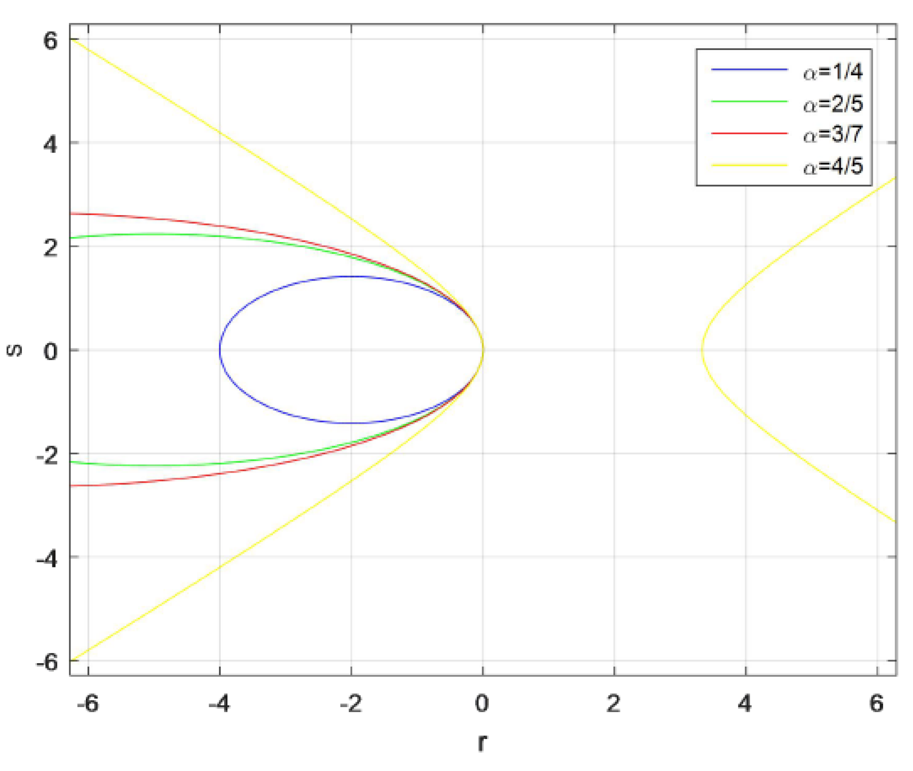
Select , , which satisfy Theorem 2; thus Equation (8) is stable in MS. Applying the semi-implicit Euler scheme, take , respectively. According to Theorem 4, the corresponding MS stability regions are depicted in Figure 1 by using Matlab software.
It is observed from Figure 1 that when , the semi-implicit fuzzy Euler scheme is not MS stable. In addition, when , according to Theorem 6, the semi-implicit fuzzy Euler scheme is absolutely unstable, thus Theorem 4 is verified; when , the semi-implicit fuzzy Euler scheme is not MS stable; when , the semi-implicit Euler scheme is MS stable; when , the semi-implicit fuzzy Euler scheme is MS stable. In short, the region of MS stability of the semi-implicit fuzzy Euler scheme is larger with the bigger value of .
5.2. Stability of Three Fuzzy Euler Scheme
In this subsection, the MS stability and asymptotical stability of the fuzzy Euler methods are verified by numerical experiments.
- (1)
- Asymptotical stability
Take the test equation as follows
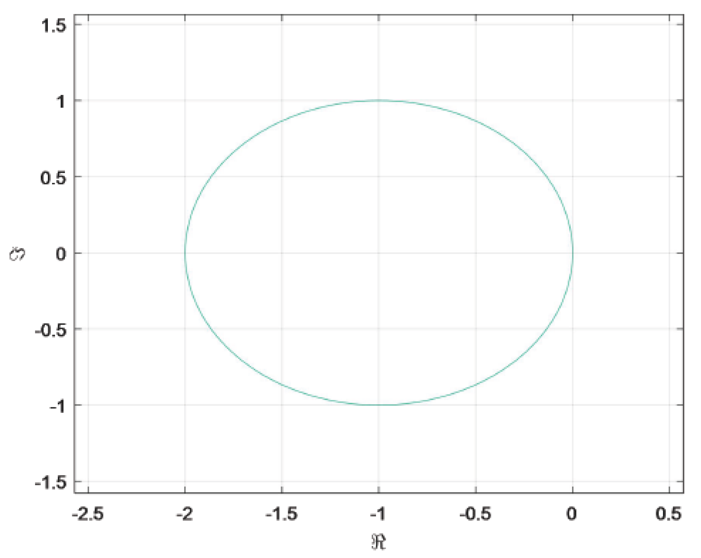
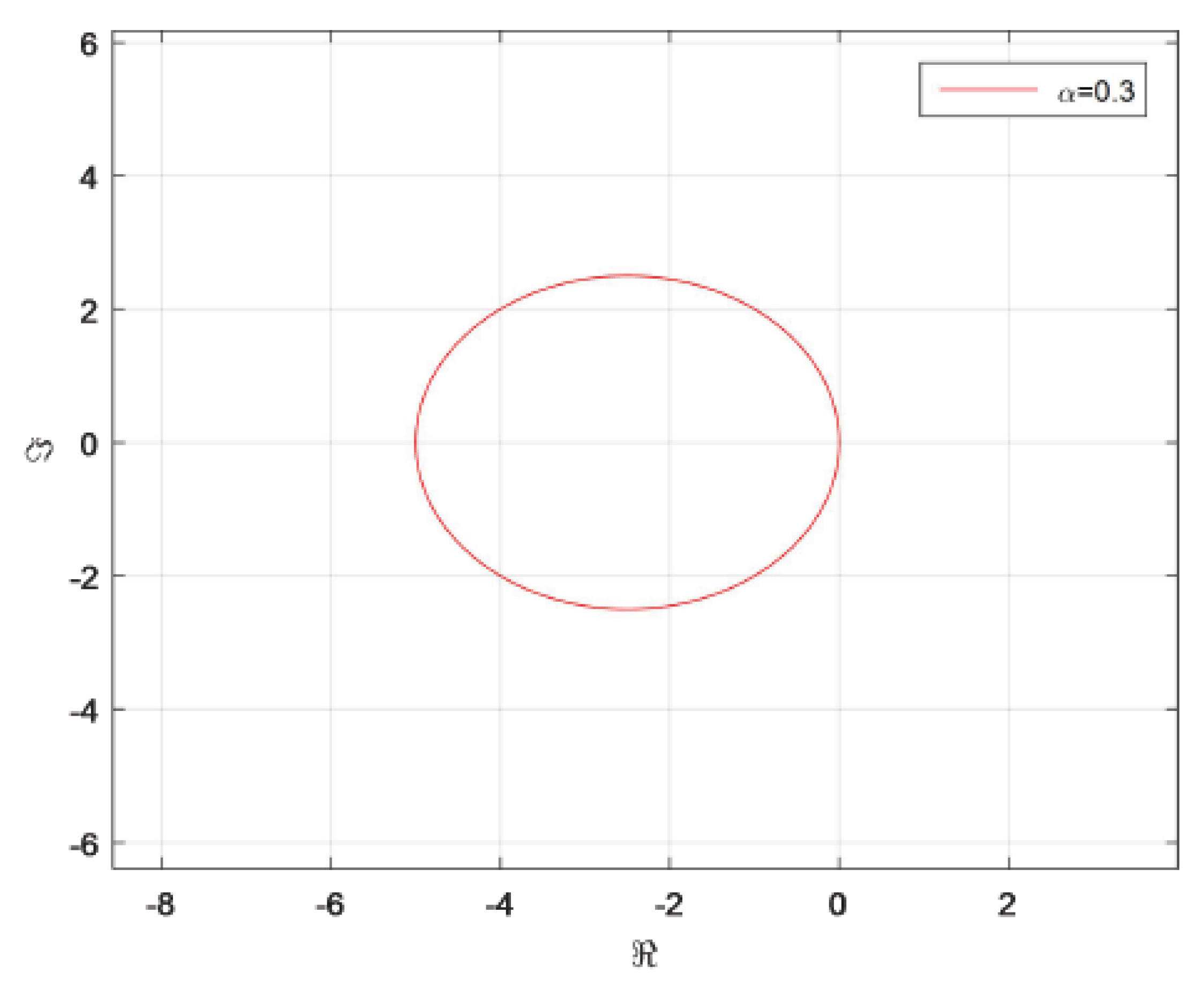
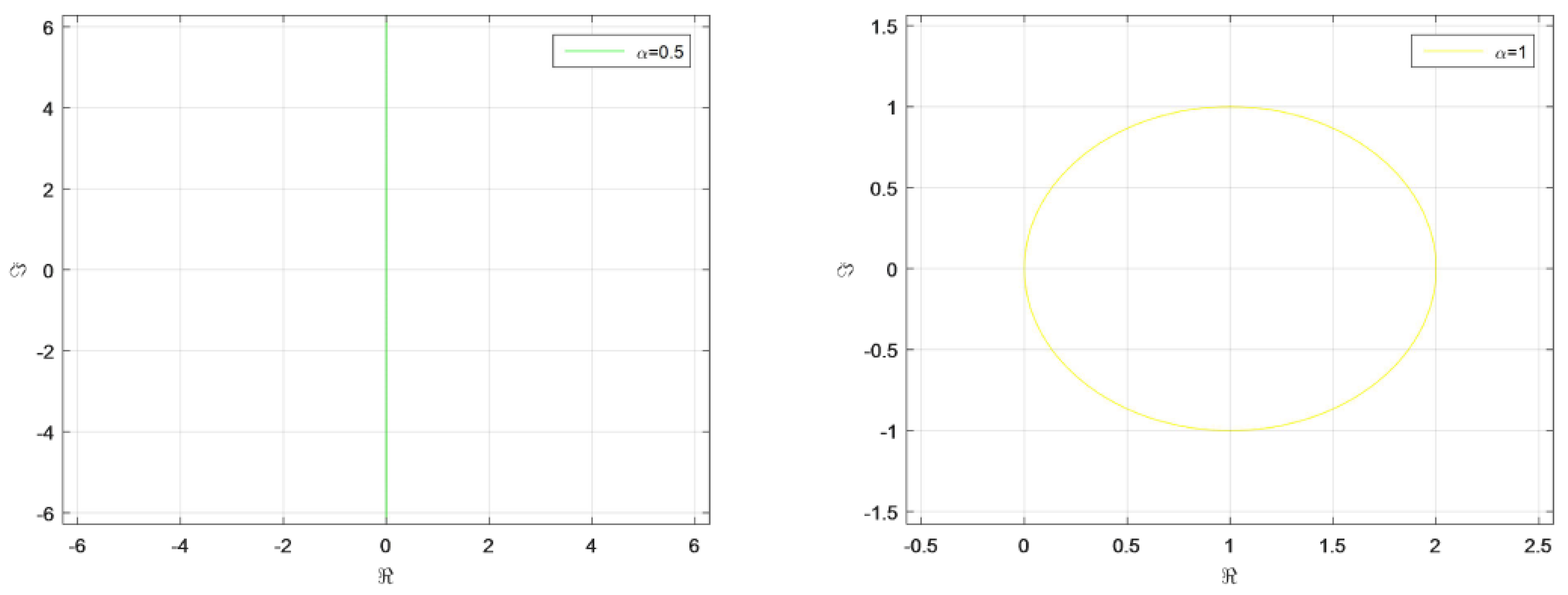
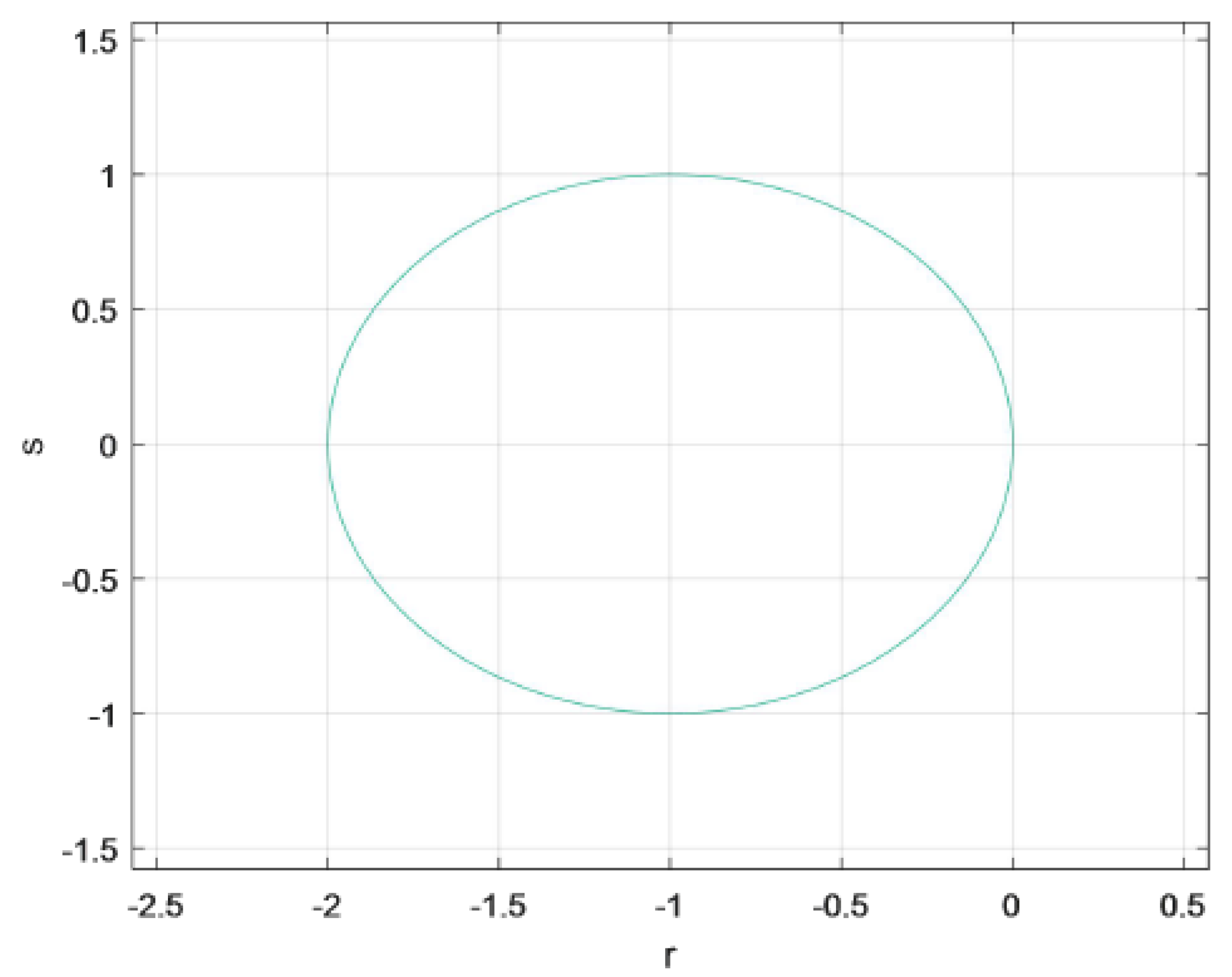
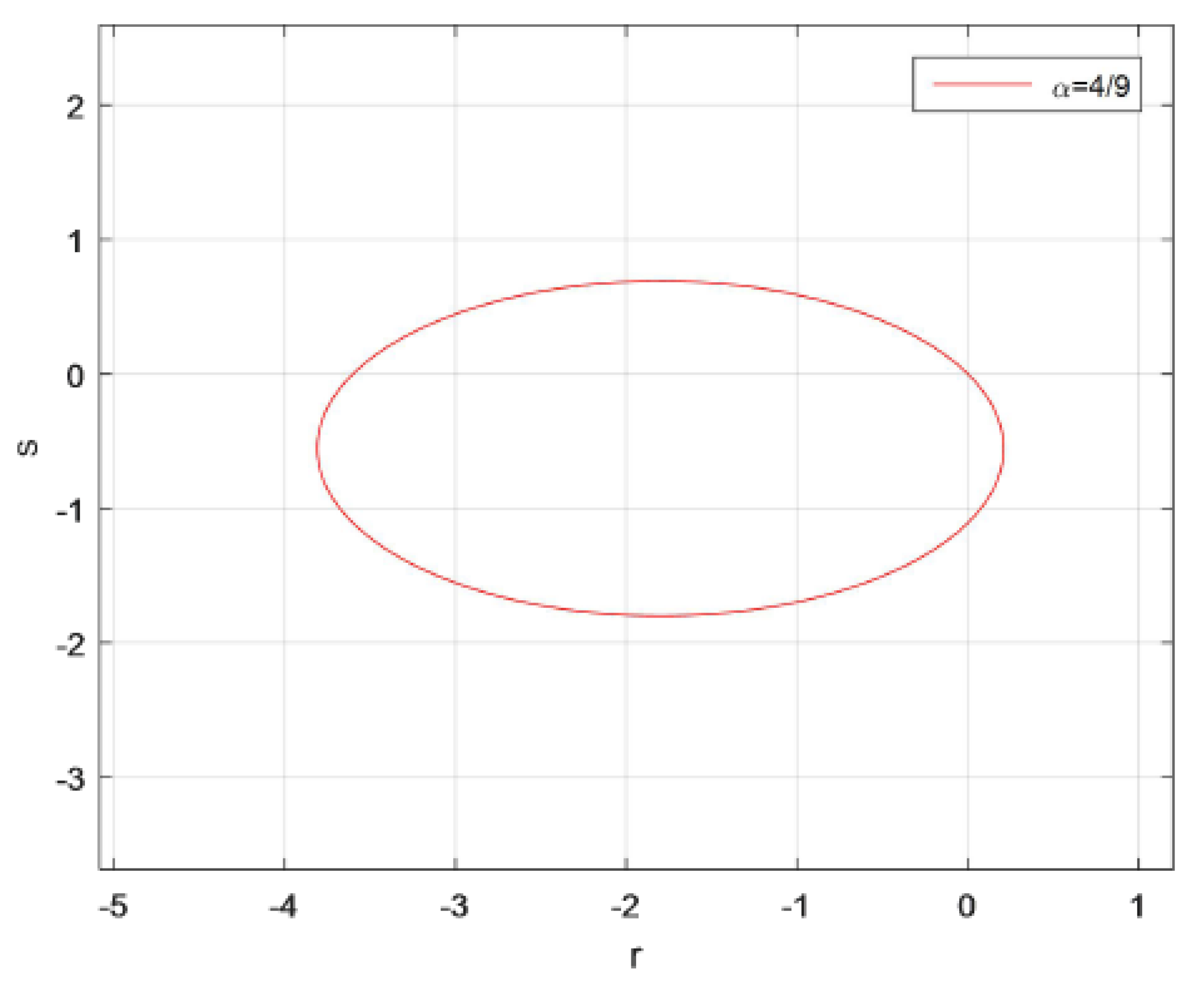
Since the region of the implicit fuzzy Euler method coincides with that of the semi-implicit fuzzy Euler scheme when , we only use the explicit fuzzy Euler schemes and the semi-implicit fuzzy Euler scheme to iterate, and take in the semi-implicit fuzzy Euler scheme to be , respectively. It follows from Section 4.1 that there is no s involved in the asymptotical stable functions , and we divide r into the real part ℜ and imaginary part ℑ. Then, the stable region of the explicit fuzzy Euler method is . Similarly, we can deduce the stable region expressed by ℜ and ℑ of the semi-implicit fuzzy Euler method based on Theorem 3. Then, the patterns of the region of asymptotical stability are given in Figure 2, Figure 3 and Figure 4. The stable region of the explicit fuzzy Euler method is the interior of the circle in Figure 2, the stable region of the semi-implicit fuzzy Euler method is the intersection of the left half plane and the exterior of the circles in Figure 3 and the right figure in Figure 4, and the stable region of the semi-implicit fuzzy Euler method is the left half plane in the left figure in Figure 4.
We find that when , the stable region of the semi-implicit fuzzy Euler scheme is larger than that of the explicit fuzzy Euler scheme; then, the stability is stronger. Therefore, for (9), the asymptotical stability of the semi-implicit fuzzy Euler scheme is better than that of the explicit fuzzy Euler scheme. Integrating Figure 1, we conclude that the implicit method has the best stability properties except for the case of the value of normal fuzzy variable is in the neighborhood of .
- (2)
- MS stability
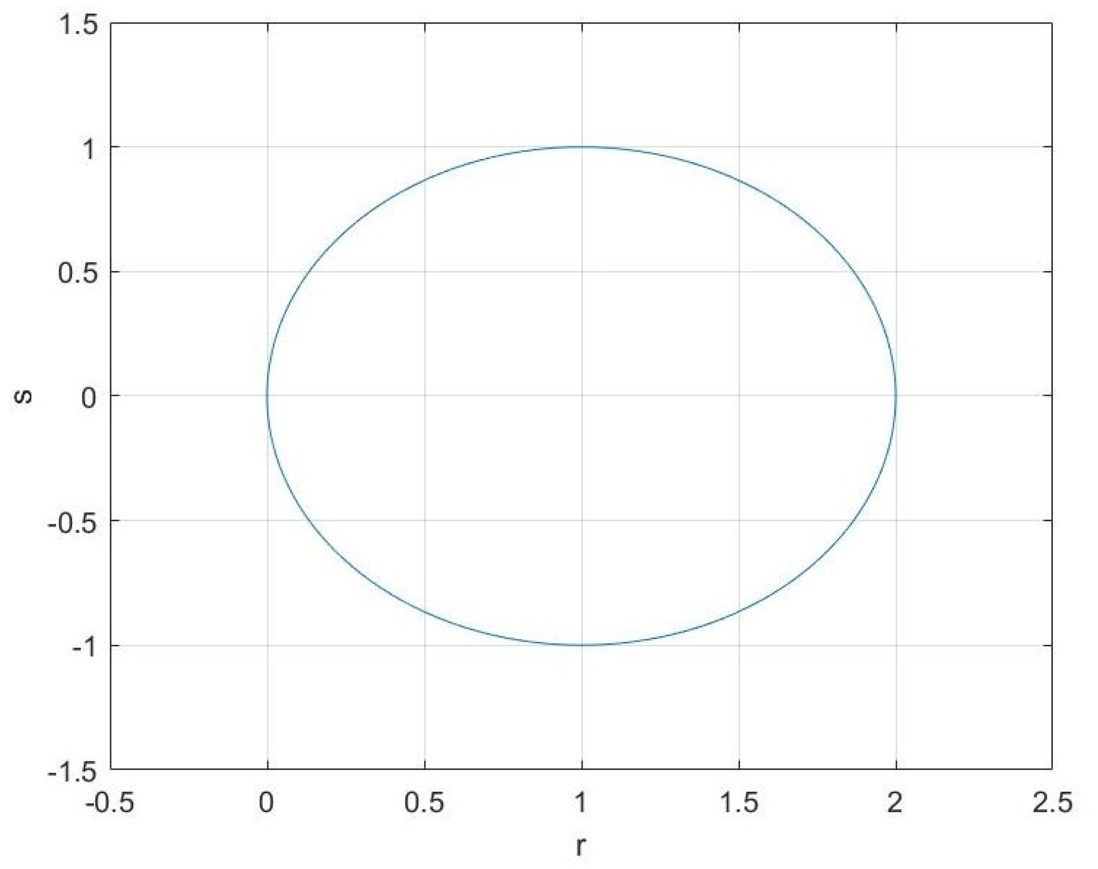
Continuing to use (8) as the test equation, three fuzzy Euler schemes are used to iterate, according to Section 4.2, their MS stable regions are shown in Figure 5, Figure 6 and Figure 7 by Matlab software. Since we have the stable region of the implicit fuzzy Euler scheme as Therefore, the stable region of the implicit fuzzy Euler scheme is the exterior of the circle in Figure 7, while the stable region of the explicit fuzzy Euler scheme and the semi-implicit fuzzy Euler scheme are the interior of the circle in Figure 5 and Figure 6.
We find that when , the stable region of the semi-implicit fuzzy Euler scheme is larger than the explicit fuzzy Euler scheme, and the stable region of the implicit fuzzy Euler scheme is the biggest. Therefore, for (8), the MS stability of the semi-implicit fuzzy Euler scheme is better than that of the explicit fuzzy Euler scheme, and the implicit method has the best stability properties except in the case in which the value of the normal fuzzy variable is in the neighborhood of .
6. Conclusions
In this paper, we gave definitions of asymptotical stability, MS stability, exponential stability and A stability, and obtained that MS stability and exponential stability are equivalent. The stability properties of fuzzy Euler methods were studied via the linear test equations. The comparison of the stabilities of three fuzzy Euler methods are listed in Table 1.
Note that, in Table 1, the implicit fuzzy Euler scheme expresses the implicit fuzzy Euler scheme where is out of the neighborhood of and the implicit fuzzy Euler scheme expresses the implicit fuzzy Euler scheme where is in the neighborhood of .
Author Contributions
Conceptualization, C.Y. and Y.C.; methodology, H.M.; software, H.M.; validation, C.Y., Y.C. and H.M.; formal analysis, Y.C.; resources, C.Y. and Y.C.; writing—original draft preparation, C.Y. and H.M.; writing—review and editing, C.Y.; supervision, C.Y. and H.M.; funding acquisition, C.Y., Y.C. and H.M.; All authors have read and agreed to the published version of the manuscript.
Funding
This research was funded by Science and Technology Project of Hebei Education Department grant number ZD2020172 and QN2020124.
Acknowledgments
The authors would like to thank the reviewers and editors for their valuable suggestions and comments, which have made a substantial improvements in this manuscript.
Conflicts of Interest
The authors declare no conflict of interest.
References
- Ngo, V.H. The initial value problem for interval-valued second-order differential equations under generalized H-differentiability. Inf. Sci. 2015, 311, 119–148. [Google Scholar]
- Zhang, S.; Sun, J. Stability of fuzzy differential equations with the second type of Hukuhara derivative. IEEE Trans. Fuzzy Syst. 2015, 23, 1323–1328. [Google Scholar] [CrossRef]
- Khastan, A.; Perfilieva, I.; Alijani, Z. A new fuzzy approximation method to Cauchy problems by fuzzy transform. Fuzzy Sets Syst. 2016, 288, 75–95. [Google Scholar] [CrossRef]
- Khastan, A.; Alijani, Z.; Perfilieva, I. Fuzzy transform to approximate solution of two-point boundary value problems. Math. Methods Appl. Sci. 2017, 40, 6147–6154. [Google Scholar] [CrossRef]
- Allahviranloo, T.; Gouyandeh, Z.; Armand, A. A full fuzzy method for solving differential equation based on Taylor expansion. J. Intell. Fuzzy Syst. 2015, 29, 1039–1055. [Google Scholar] [CrossRef]
- Alijani, Z.; Baleanu, D.; Shiri, B.; Wu, G.C. Spline collocation methods for systems of fuzzy fractional differential equations. Chaos, Solitons Fractals 2020, 131, 109510. [Google Scholar] [CrossRef]
- Nematollah, K.; Sedigheh, S.R.; Hossein, J. Differential transform method: A tool for solving fuzzy differential equations. Int. J. Appl. Comput. Math. 2018, 4, 33. [Google Scholar]
- Chehlabi, M. Continuous solutions to a class of first-order fuzzy differential equations with discontinuous coefficients. Comput. Appl. Math. 2018, 37, 5058–5081. [Google Scholar] [CrossRef]
- Khastan, A.; Rodrguez-Lpez, R. On linear fuzzy differential equations by differential inclusions’ approach. Fuzzy Sets Syst. 2020, 387, 49–67. [Google Scholar] [CrossRef]
- Mosleh, M.; Otadi, M. Approximate solution of fuzzy differential equations under generalized differentiability. Appl. Math. Model. 2015, 39, 3003–3015. [Google Scholar] [CrossRef]
- Soheil, S.; Ali, A.; Animesh, M.; Sankar, P.M.; Shariful, A. The behavior of logistic equation with alley effect in fuzzy environment: Fuzzy differential equation approach. Int. J. Appl. Comput. Math. 2018, 4, 62. [Google Scholar]
- Liu, B.; Liu, Y.K. Expected value of fuzzy variable and fuzzy expected value models. IEEE Trans. Fuzzy Syst. 2002, 10, 445–450. [Google Scholar]
- Liu, B. Fuzzy process, hybrid process and uncertain process. J. Uncertain Syst. 2008, 2, 3–16. [Google Scholar]
- Dai, W. Lipschitz continuity of Liu process. In Proceedings of the 8th International Conference on Information and Management Science, Kunming, China, 20–28 July 2009; pp. 756–760. [Google Scholar]
- You, C.; Huo, H.; Wang, W. Multi-dimensional Liu process, differential and integral. East Asian Math. J. 2013, 29, 13–22. [Google Scholar] [CrossRef] [Green Version]
- Zhu, Y. Stability analysis of fuzzy linear differential equations. Fuzzy Optim. Decis. Mak. 2010, 9, 169–186. [Google Scholar] [CrossRef]
- You, C.; Hao, Y. Stability in mean for fuzzy differential equation. J. Ind. Manag. Optim. 2019, 15, 1375–1385. [Google Scholar] [CrossRef]
- You, C.; Hao, Y. Stability in credibility for fuzzy differential equation. J. Intell. Fuzzy Syst. 2019, 36, 213–218. [Google Scholar] [CrossRef]
- You, C.; Hao, Y. Fuzzy Euler approximation and its local convergence. J. Comput. Appl. Math. 2018, 343, 55–61. [Google Scholar] [CrossRef]
- Cheng, Y.; You, C. Convergence of numerical methods for fuzzy differential equations. J. Intell. Fuzzy Syst. 2020, 38, 5257–5266. [Google Scholar] [CrossRef]
- Zhu, Y. A fuzzy optimal control model. J. Uncertain Syst. 2009, 3, 270–279. [Google Scholar]
- Qin, Z.; Bai, M.; Dan, R. A fuzzy control system with application to production planning problems. Inf. Sci. 2011, 181, 1018–1027. [Google Scholar] [CrossRef]
- Liu, B. Uncertainty Theory, 2nd ed.; Springer: Berlin/Heidelberg, Germany, 2007. [Google Scholar]
Figure 1.
The region of MS stability of semi-implicit fuzzy Euler scheme.

Figure 2.
The region of asymptotical stability of explicit fuzzy Euler scheme.

Figure 3.
The region of asymptotical stability of semi-implicit fuzzy Euler scheme.

Figure 4.
The region of asymptotical stability of semi-implicit fuzzy Euler scheme.

Figure 5.
The region of MS stability of explicit fuzzy Euler scheme.

Figure 6.
The region of MS stability of semi-implicit fuzzy Euler scheme.

Figure 7.
The region of MS stability of implicit fuzzy Euler scheme.


Table 1.
Stabilities of three fuzzy Euler methods.
| Stabilities | Asymptotical Stability | MS Stability Exponential Stability | A Stability |
|---|---|---|---|
Publisher’s Note: MDPI stays neutral with regard to jurisdictional claims in published maps and institutional affiliations. |
© 2022 by the authors. Licensee MDPI, Basel, Switzerland. This article is an open access article distributed under the terms and conditions of the Creative Commons Attribution (CC BY) license (https://creativecommons.org/licenses/by/4.0/).
Share and Cite
MDPI and ACS Style
You, C.; Cheng, Y.; Ma, H. Stability of Euler Methods for Fuzzy Differential Equation. Symmetry 2022, 14, 1279. https://0-doi-org.brum.beds.ac.uk/10.3390/sym14061279
AMA Style
You C, Cheng Y, Ma H. Stability of Euler Methods for Fuzzy Differential Equation. Symmetry. 2022; 14(6):1279. https://0-doi-org.brum.beds.ac.uk/10.3390/sym14061279
Chicago/Turabian StyleYou, Cuilian, Yan Cheng, and Hongyan Ma. 2022. "Stability of Euler Methods for Fuzzy Differential Equation" Symmetry 14, no. 6: 1279. https://0-doi-org.brum.beds.ac.uk/10.3390/sym14061279
Note that from the first issue of 2016, this journal uses article numbers instead of page numbers. See further details here.