A Joint Positioning Algorithm in Industrial IoT Environments with mm-Wave Communications

Abstract

With the real restriction of packet size and transmission power, a joint UL-AoA (Uplink Angle of Arrival) and UL-TDOA (Uplink Time Difference of Arrival) positioning method is discussed for the Industrial Internet of Things (IIoT), which demands high accuracy of position information. One motivation of the UL positioning method of IIoT is an asymmetric network and uplink traffic is dominant in most identified scenarios. Further, IIoT sensors are power limited for low cost, compared to the transmission power of base stations and other normal user equipment. This paper considers an environment of a 5G-enabled IIoT network with massive Multiple input multiple output (MIMO) antennas, beamforming and millimeter operating bands. After reviewing downlink positioning reference signal (PRS) and uplink sounding reference signal for positioning (SRS-Pos), a general system model and a theoretical localization problem is derived under the joint positioning method. The provided simulation results help to investigate the impact of system configurations on positioning measurements. Further, through the test in this paper, it is proved that joint positioning outperforms that of the time only or angle only method.

1. Introduction

A 5G system puts forward stricter requirements on positioning accuracy and performance of user equipment (UE) position than a 4G wireless cellular communication network system. The confidence of positioning accuracy of each positioning performance level is 95% [1]. This means that 3GPP will deeply couple 5G communication and positioning capabilities and continue to add value to 5G-enabling vertical industries.

The Industrial Internet of Things is a major vertical focus area for NR R16 [2,3], and is shaping the future of many commercial applications. The fourth Industrial Revolution (Industry 4.0) triggered by IIoT will bring significant revenue expansion through the new digital service provider market [4]. The IIoT network will be scalable in terms of connections and number of devices and will use key LTE and 5G new radio (NR) capabilities, such as ultra-reliable low-delay communication, large-scale machine-type communication, 5G positioning, time-sensitive communication, and to a lesser extent, enhanced mobile broadband.

In Industry 4.0, there is a growing need to develop indoor navigation and localization systems for future living and working environments. The market opportunities of Indoor-Localization-related systems are expected to be in the order of USD 10 billion by 2024 [5]. The presence of 5G has the potential to improve indoor positioning estimation to sub-meter accuracy [6] and offers opportunities for a large number of applications in manufacturing [7].

In the R16 version, 5G can achieve an indoor positioning accuracy of 3 m and outdoor positioning accuracy of 10 m [8]. The R16 can achieve accuracy of less than 5 m outdoors and less than 3 m indoors by using high time resolution of 5G bandwidth and multi-beam Angle information. However, there is still a gap between centimeter-level high-precision positioning requirements. In R17, critical 5G positioning capabilities will be improved to meet the needs of more stringent use cases such as centimeter-level accuracy, while reducing positioning delay and increasing positioning efficiency to expand capacity [1]. Low power devices with high accuracy positioning (LPHAP) is one of the enhanced features of R18 defined 5G-Advanced [9], which includes sub-meter accuracy to further reduce latency and terminal power consumption, enabling 5G positioning to meet the requirements for higher accuracy and delay in more end markets [6,10], as summarized in

Table 1. Positioning accuracy requirement in NR System.

Release	Bandwidth	Positioning Accuracy
R16	100 MHz	1–3 m
R17	100 MHz	0.5 m
R18	200–800 MHz	10 cm

.

This illustrates the areas that the strict requirements of IIoT for 5G cellular positioning with higher precision, richer terminal types, and significantly reduced terminal side power consumption are further focused on. Among the numerous requirements, the most important one is to reduce the power consumption of the positioning device while maintaining the positioning accuracy, so as to occupy the growing positioning market and expand the potential IIoT Settings use cases, supporting the need to add new use cases, such as factory automation and power distribution.

2. Related Work

Support for a variety of location technologies to provide reliable and accurate user location has been a key research area of the 3GPP standard. The authors of [11], introduce a downlink angle of departure (DL-AoD) and an uplink angle of arrival (UL-AoA), multi-round trip time (Multi-RTT), downlink time difference of arrival (DL-TDOA), uplink time difference of arrival (UL-TDOA), and other new positioning measurement methods. It greatly expands the positioning mode supported by the 5G system and makes up for the deficiency that R15 does not support positioning using NR signals and improves the performance of UE positioning, especially in indoor environments where GNSS cannot work normally. In R16, the used reference signal for positioning are PRS and SRS-Pos for downlink measurement and uplink measurement, respectively.

The main principle of TDOA is to calculate the UE position by constructing a nonlinear hyperbolic equation, wherein a distance difference between every two base stations to a single UE is modeled according to the signal arrival time difference. There are many kinds of literature to investigate various methods to obtain signal arrival time difference for TDOA localization, such as the cross-correlation algorithm using received signal and transmitted signal [12], based on timing advance (TA) value to obtain the signal arrival time difference [13], etc. However, one disadvantage of these methods is that the phase characteristics of the system cannot be obtained, and it is sensitive to additional signals.

AoA is a positioning algorithm based on the angle of arrival of signals. UE positioning is carried out by measuring the azimuth angle of arrival (A-AoA) and the zenith angle of arrival (Z-AoA), which can be configured on the network side [11]. The proposed positioning methods in [14,15] were based on MIMO (multi input multi output) technology and greatly improve the positioning accuracy. In [16], the author studies the characteristics of time-frequency signals and uses the orthogonality of signal and noise subspace to obtain more accurate angle estimation results. Once the signal arrives, some references provide specific methods for calculating UE coordinates from angle estimates. For example, in [17] the author introduces the modified polar representation to calculate the localization of a ue using AoA, and in [18], the author proposes a closed-form solution for 3D localization using AoAs.

For such TDOA- or AoA-only positioning methods, there are some disadvantages. The positioning accuracy of AoA is very dependent on the angle measurement accuracy of the array antenna and is sensitive to signal propagation distance. TDOA has high positioning accuracy, but is seriously affected by channel uncertainty. Therefore, a mixture of multiple positioning methods can be considered. In the existing studies, the fusion of localization schemes mainly includes TDOA + AoA and TDOA/AoA + fingerprints [19,20,21,22,23]. The combination of TDOA and AoA can better solve the synchronization problem in a time-based positioning scheme and the problem that the angle-based positioning scheme is sensitive to the rotation angle of the device.

In the scenario of IIoT, higher requirements are put forward for positioning accuracy and power consumption of positioning equipment. In [24], the author proposes a big-data-driven method to improve positioning accuracy by analyzing the data of low-power beacons and scanners to detect the indoor position of users in a specific “activity-based area” during the activities of daily life. However, such a method requires higher signal processing capability on the sensors. In [25], the author aims to evaluate the positioning performance in terms of accuracy and availability while considering different deployment strategies. To reduce the power consumption of positioning devices, in [26], the author provides a wireless IoT device alliance based on the framework of common interests, energy and physical awareness, which improve the energy efficiency of the whole system, reduce power consumption, and extend the battery life of the equipment. In [27], the author proposes an LPHAP solution under the framework of the 3GPP NR standard. The research and development of LPHAP technology provide key support for solving the bottleneck problem of IIoT application development, and currently, related research is quite limited.

The purpose of this paper is to provide a joint UL-AoA and UL-TDOA for IIoT sensors positioning with a constriction of resource overhead, power restriction, and traffic condition, according to the real IIoT environment [1,7]. That is to say, an asymmetric IIoT network is considered in this paper. IIoT sensors are power restricted and can sustain a long lifetime without changing the battery (typically, this could be 1–2 years). Further, uplink traffic is dominant according to identified scenarios [2]. The resource overhead for positioning is analyzed in this paper. The work in this paper assumes a millimeter wave communication supporting a finer delay domain resolution, and presents the corresponding test results after giving an overview of PRS and SRS-Pos design. Our simulation-based evaluation shows that network configuration plays a vital role when it comes to achieving a high-accuracy positioning performance, and the joint positioning method outperforms the AoA only and TDOA only.

The rest of this paper is organized as follows. In Section 3, DL PRS and UL SRS-Pos are reviewed. Then, the proposed algorithm for IIoT is described in Section 4. Section 5 presents the test results, and the conclusion is drawn in Section 6. For easy description and reading, some notations are summarized in

Table 2. Notation description.

Notation	Explanation
$L_{\mathrm{PRS}}$	consecutive OFDM symbols within a slot in time domain
$K_{\mathrm{comb}}^{\mathrm{PRS}}$	frequency granularity of PRS resources
$n_{\mathrm{SRS}}^{\mathrm{cs},\max }$	maximum number of cyclic shifts
$K_{\mathrm{TC}}^{\mathrm{SRS}}$	comb structure of transmitted SRS-Pos
${\mathbb{C}}^{m\times n}$	a set of $m\times n$ dimensional complex matrix
${\left(·\right)}^{†}$	conjugate transpose operation
${\left(·\right)}^T$	transpose operation
$N_{\mathrm{RE}}^{\mathrm{SRS}}$	SRS RE number
$N_{\mathrm{RB}}^{\mathrm{PRS}}$	PRS RB number
$N_{\mathrm{RB}}^{\mathrm{SRS}}$	SRS RB number
$\mathcal{C}\mathcal{N}\left(\mu ,{\sigma }^2\right)$	normal distribution with mean $\mu$ and variance ${\sigma }^2$
$\mathbf{I}$	identity matrix
$\mathrm{E}\{·\}$	the expectation operation
$\mathcal{O}\left(·\right)$	time complexity
${\Xi }_{\mathrm{TDOA}}$	the algorithm complexity of UL-TDOA
${\Xi }_{\mathrm{AoA}}$	the algorithm complexity of UL-AoA
${\Xi }_{\mathrm{joint}}$	the algorithm complexity of joint UL-AoA + TDOA

.

3. Overview of NR PRS and SRS-Pos Design

3.1. DL Positioning Reference Signal, DL-PRS

In the DL positioning technology scheme (mainly based on DL-TDOA or DL-AoD), and the uplink-downlink joint positioning technology scheme, UE obtains the measurement value by detecting the PRSs from multiple base stations or transmission/reception points (TRPs). As a tradeoff of signaling overhead and flexible resource allocation under multiple TRP non-colliding transmissions to position a device, NR uses a hierarchy with positioning frequency layers, PRS resource sets and PRS resources to define the structure, as shown in Figure 1a. One positioning frequency layer consists of one or more PRS resource sets across one or more TRPs, all with the same carrier frequency, subcarrier spacing (SCS, i.e., OFDM numerology), PRS bandwidth and so on. A PRS resource set contains at most two PRS resources originating from the same TRP, and parameters comprising PRS repetition factor, resource offset, etc., are identical. Each PRS resource typically corresponds to a beam from the TRP. Then, by configuring a device to measure on a certain PRS resource from a PRS resource set, the location server obtains knowledge not only about which TRP the reported measurements correspond to, but also the particular beam from the TRP.

For each PRS transmission, a frequency-time resource set with $L_{\mathrm{PRS}}\in \left\{2,4,6,12\right\}$ consecutive OFDM symbols within a slot in time domain and $N_{\mathrm{RB}}^{\mathrm{PRS}}\in \left\{28,32,\dots ,272\right\}$ consecutive PRBs (Physical Resource Blocks) in the frequency domain is used. Note that the frequency resources are configured with a granularity of four PRBs [28].

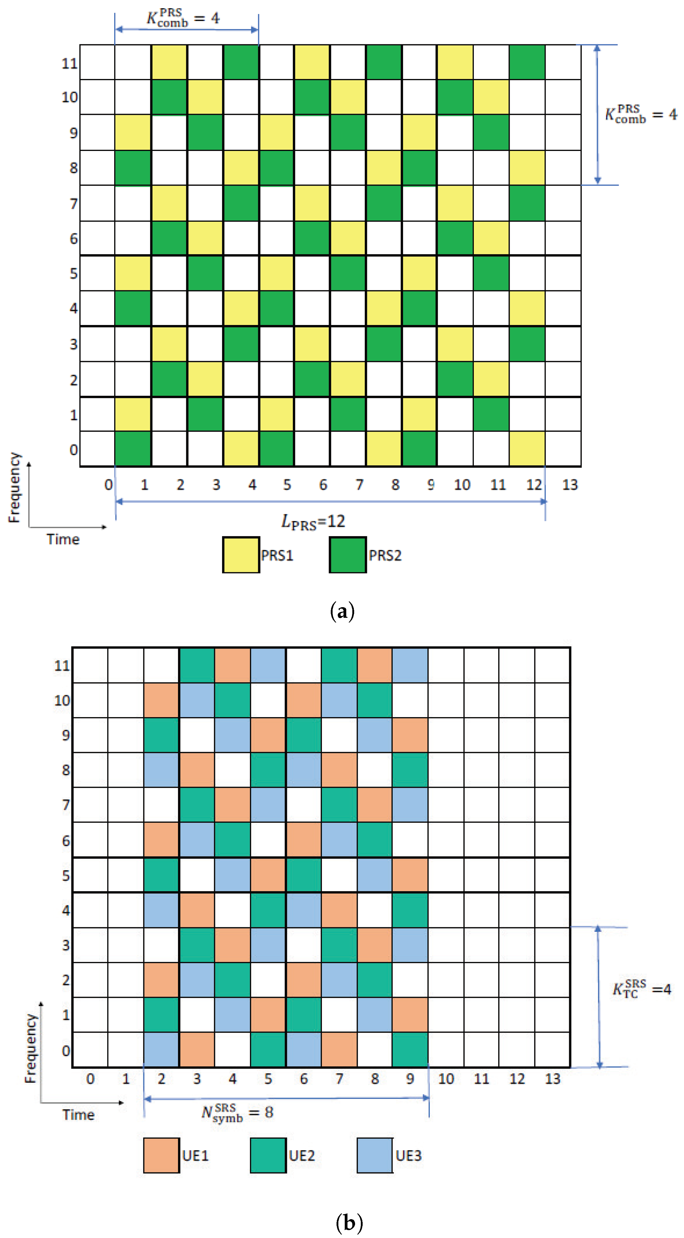
Further, to allow simultaneous transmission of multiple PRS, a comb-based transmission is designed. $K_{\mathrm{comb}}^{\mathrm{PRS}}\in \left\{2,4,6,12\right\}$ is the frequency granularity of PRS resources, i.e., the PRS utilizes every $K_{\mathrm{comb}}^{\mathrm{PRS}}$th subcarrier. Then, one device should listen to multiple TRPs for positioning. Figure 2a shows an example of PRS time-frequency resource element (RE) mapping under a comb-based design with $K_{\mathrm{comb}}^{\mathrm{PRS}}=4$ and $L_{\mathrm{PRS}}=12$.

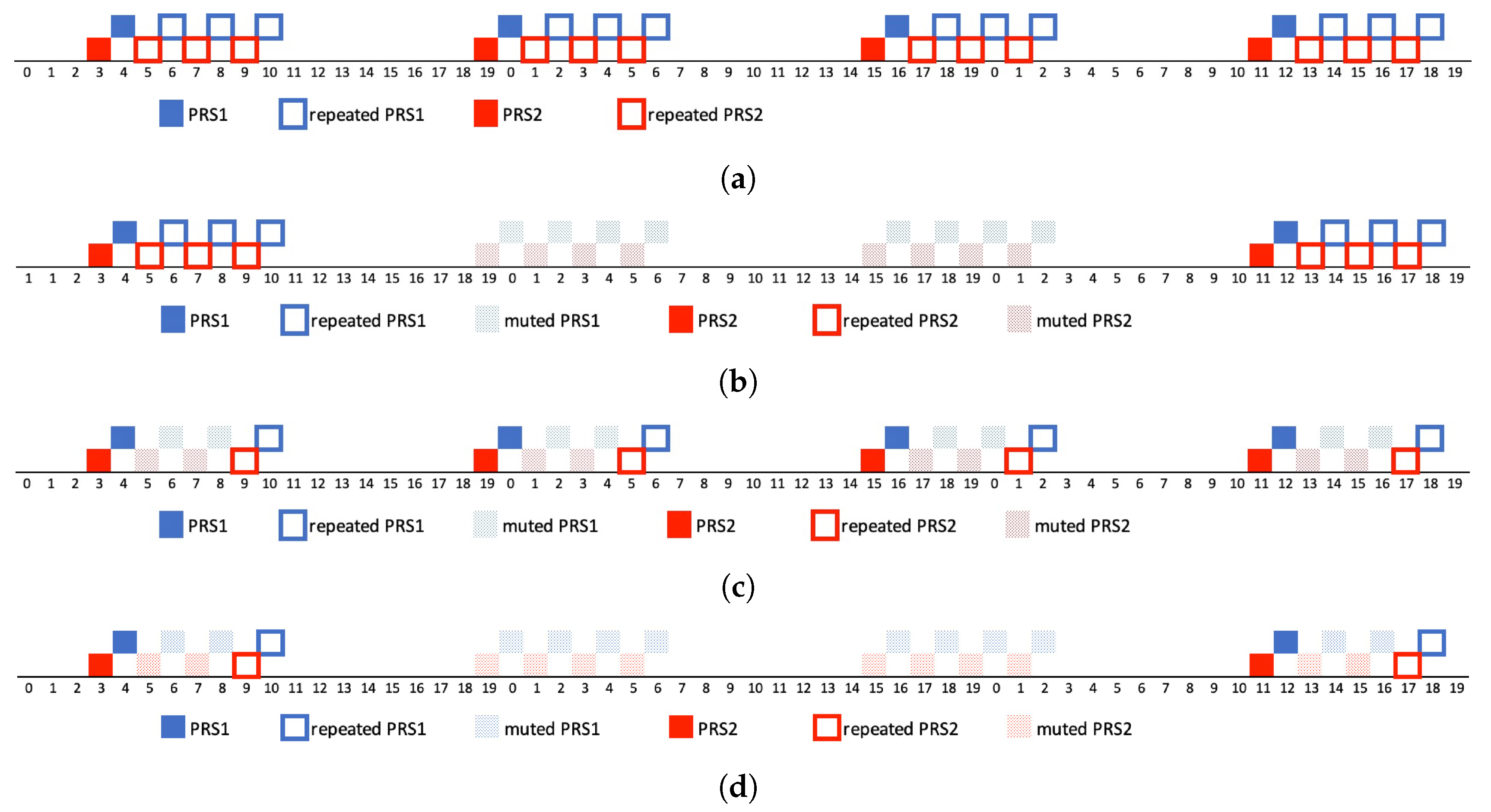
Apart from the resource coordination, another near–far issue must be accounted for, since the device also needs to listen to PRSs from more distant TRPs. There is no sufficient dynamic range in the receiver to handle both a relatively weak signal from a distant TRP and a strong signal from a more closely located TRP simultaneously. Therefore, a mechanism to ensure that the near TRP is silent while measuring on the distant TRP is required. In NR system, such a requirement is achieved by specifying muting option1 (i.e., Opt1) and option2 (i.e., Opt2) through different bitmaps. When a bit in the bitmap is zero, the PRSs at the corresponding time instants are not transmitted. For Opt1, one bit corresponds to one PRS transmission period, while corresponding to one PRS repeated transmission within each PRS period for Opt2. Application of Opt1 and Opt2 simultaneously in NR system to mute not only a repeated instant but also a periodic instant is allowed.

Several examples under different muting patterns are provided in Figure 3. Example (a) is a normal PRS transmission without muting. Example (b) represents PRS1 and PRS2 transmission under muting Opt1 with a bitmap $\left\{1,0,0,1\right\}$. Then, the PRS transmission in the second and the third periods are muted. Under the same bitmap with Example B, the second and third repeated PRS transmission within each period are muted in Example (c) with a muting Opt2. By combining Opt1 and Opt2, the second and third repeated PRS instants of each period are muted, while the second and third periods are also muted in Example (d).

3.2. UL Positioning Reference Signal, UL SRS-Pos

UL SRS-Pos is used to provide the positioning measurement for UL-TDOA, UL-AoA and Multi-RTT. These measurements include UL RTOA, UL-AoA (including A-AoA and Z-AoA), reference signal received power (RSRP), and TRP transmission time differences.

Considering the UL link restriction, SRS-Pos is a zadoff-chu sequence [14], due to the good autocorrelation, low cross-correlation and low peak to average power ratio (PAPR) characteristics. It is expressed as

$$\begin{array}{c}\hfill \left\{\begin{array}{c}{\mathbf{r}}_{\text{SRS-Pos}}={\mathbf{r}}_{u,v}^{\left({\alpha }_i,\delta \right)}\hfill \\ {\alpha }_i=2\pi n_{\mathrm{SRS}}^{\mathrm{cs},\mathrm{i}}/\phantom{n_{\mathrm{SRS}}^{\mathrm{cs},i}{n}_{\mathrm{SRS}}^{\mathrm{cs},\max }}{n}_{\mathrm{SRS}}^{\mathrm{cs},\max }\hfill \\ \delta ={log}_2\left(K_{\mathrm{TC}}^{\mathrm{SRS}}\right)\hfill \end{array}\right.,\end{array}$$

(1)

where ${\alpha }_i$ represents a cyclic shift of port; $n_{\mathrm{SRS}}^{\mathrm{cs},\max }$ is the maximum number of cyclic shifts; $n_{\mathrm{SRS}}^{\mathrm{cs},\mathrm{i}}\in \left\{0,1,\dots ,n_{\mathrm{SRS}}^{\mathrm{cs},\max }-1\right\}$; $K_{\mathrm{TC}}^{\mathrm{SRS}}\in \left\{2,4,8\right\}$ represents SRS-Pos comb size, which means that SRS-Pos is transmitted in a comb structure to support multi-user multiplexing within the same set of time-frequency resources, i.e., the number of multiplexed UE is $K_{\mathrm{TC}}^{\mathrm{SRS}}$.

Regarding the time-frequency resource allocation for SRS-Pos, one SRS-Pos resource occupies multiple consecutive OFDM symbols in the time domain to guarantee the performance, and the symbol number is $N_{\mathrm{symb}}^{\mathrm{SRS}}\in \left\{1,2,4,8,12\right\}$. In the frequency domain, SRS-Pos can be configured up to $N_{\mathrm{PRB}}^{\mathrm{SRS}}=272$ consecutive PRBs with a granularity of four PRBs [14]. Figure 2b shows an example of SRS-Pos comb-based RE mapping with $K_{\mathrm{TC}}^{\mathrm{SRS}}=4$ and $N_{\mathrm{symb}}^{\mathrm{SRS}}=8$, and it can be founded that SRS-Pos resource is a permuted staggered comb, i.e., the starting positions of a single SRS-pos in different OFDM symbols are different to provide a possibility of coherent combination at the receiver side. Such a design is similar to PRS.

Further, SRS-Pos transmission can be semi-continuous, periodic, and aperiodic, according to demand and UE capabilities. In case of semi-continuous transmission, TRP can dynamically activate or deactivate SRS-Pos. In case of periodical SRS-Pos, UE starts SRS-Pos transmission once the corresponding configuration is available. In case of aperiodic SRS-Pos, TRP triggers each SRS-Pos transmission by DCI (downlink control information). Whether a UE supports aperiodic SRS-Pos transfers depends on the UE capabilities.

Different from DL positioning, to support flexible configuration, a device can be configured with multiple SRS-Pos resource sets comprising multiple SRS-Pos resources, as shown in Figure 1b. For each SRS-Pos resource set, parameters comprising the transmission type (i.e., periodic, aperiodic and semi-continuous), transmission power are unified for multiple SRS-Pos resources. Correspondingly, to support flexible resource allocation of UL positioning according to the channel status of each UE, flexible configurations for comb size, time domain duration, PRB position in the frequency domain, and so on are allowed for each SRS-Pos resource.

3.3. Resource Overhead Analysis of DL PRS and UL SRS-Pos

According to the above description, the radio resource overhead for PRS and SRS-Pos, from the perspective of UE side, can be expressed as

$$\begin{array}{c}\hfill \left\{\begin{array}{c}{\eta }_{\mathrm{PRS}}=\frac{L_{\mathrm{PRS}}{N}_{\mathrm{RB}}^{\mathrm{PRS}}{N}_{\mathrm{TRP}}}{N_{\mathrm{symb}}^{\mathrm{system}}{N}_{\mathrm{BW}}^{\mathrm{system}}{K}_{\mathrm{comb}}^{\mathrm{PRS}}}\hfill \\ \\ {\eta }_{\text{SRS-Pos}}=\frac{N_{\mathrm{symb}}^{\mathrm{SRS}}{N}_{\mathrm{RB}}^{\mathrm{SRS}}}{N_{\mathrm{symb}}^{\mathrm{system}}{N}_{\mathrm{BW}}^{\mathrm{system}}{K}_{\mathrm{TC}}^{\mathrm{SRS}}}\hfill \end{array}\right.,\end{array}$$

(2)

where $N_{\mathrm{symb}}^{\mathrm{system}}$ denotes the system symbol number per slot and $N_{\mathrm{BW}}^{\mathrm{system}}$ is the system bandwidth.

From (2), it can be observed that resource overhead of DL positioning is a little bit larger than that of UL positioning. Another thing that should be noted is measurement reports in DL positioning will need additional UL radio resource, which requires corresponding resource allocation. The measurement port for DL positioning will also impact power consumption on the UE side. In case of DL-TDOA positioning method, the PRS overhead will be larger than that of UL, since at least three TRPs are required for exact positioning.

4. Design of Joint Positioning Algorithm

Considering the fact that UL transmission is dominant in IIoT with a limited traffic packet size as around 256 bytes [1], and much more wide bandwidth is available in mm-Wave bands [29,30], this paper proposes considering UL-based positioning for IIoT. Another consideration is UEs do not have to monitor PRS within a long duration and report the measurement results.

Then, assuming there is only one transmission antenna for a IIoT device, the received signal can be expressed as

$$\begin{array}{cc}\hfill \mathbf{Y}& =\left({\mathbf{Y}}_1,\dots ,{\mathbf{Y}}_{N_{\mathrm{TRP}}}\right)\hfill \\ \hfill & =\mathbf{H}{\mathbf{r}}_{\text{SRS-Pos}}+\mathbf{Z}\in {\mathbb{C}}^{N_{\mathrm{R}}\times N_{\mathrm{symb}}^{\mathrm{SRS}}\times N_{\mathrm{RE}}^{\mathrm{SRS}}\times N_{\mathrm{TRP}}},\hfill \end{array}$$

(3)

where $\mathbf{Y}$ denotes the received signal in frequency domain, and ${\mathbf{Y}}_i\in {\mathbb{C}}^{N_{\mathrm{R}}\times N_{\mathrm{symb}}^{\mathrm{SRS}}\times N_{\mathrm{RE}}^{\mathrm{SRS}}}$ is the received signal between the device and ith TRP; $N_{\mathrm{R}}$ is the number of receiving antenna with the assumption that the receiving antenna number is identical for each TRP; $\mathbf{Z}$ is independent circularly symmetric complex Gaussian noise as $\mathbf{Z}\sim \mathcal{C}\mathcal{N}\left(0,{\sigma }^2\right)$; $\mathbf{H}$ is the channel response between UE and all TRPs, and the ith element ${\mathbf{H}}_i\in {\mathbb{C}}^{N_{\mathrm{R}}\times N_{\mathrm{symb}}^{\mathrm{SRS}}\times N_{\mathrm{RE}}^{\mathrm{SRS}}}$ within $\mathbf{H}$ represents the SIMO (single input multiple output) channel between UE and ith TRP. Considering many obstacles in an IIoT environment wherein shadowing and pathloss cannot be ignored, a composite fading channel is assumed, and each element of ${\mathbf{H}}_i$ can be expressed as

$${\mathbf{H}}_i\left(k,l\right)=\sqrt{{\Omega }_i{\rho }_i}g,$$

(4)

where ${\mathbf{H}}_i\left(k,l\right)$ represents the channel response within ${\mathbf{H}}_i$ at kth RE and OFDM symbol l; ${\Omega }_i$ represents the shadowing effect, and is modeled by a log-normal distribution as $10log{\Omega }_i\sim \mathcal{C}\mathcal{N}\left(0,{\chi }_i^2\right)$; g is the fast fading and is assumed to follow a Rayleigh distribution; ${\rho }_i$ is the pathloss and modeled as [25]

$${\rho }_i={\left(\frac{d_{\mathrm{f}}}{d_i}\right)}^{{\beta }_i}$$

(5)

where $d_{\mathrm{f}}$ is the reference distance, $d_i$ denotes the distance from UE to the ith TRP, and ${\beta }_i$ is the path loss exponent.

Based on the received signal in (3), the signal detection for delay and angle under the joint positioning algorithm can be performed according to the following subsections. The algorithm process is shown in Figure 4.

4.1. Time Difference Estimation

To estimate the time difference between different TRPs, the core work is the accumulation of correlation power and the time domain sample position of the valid estimated RSRP. Then, RSRP at ith TRP can be obtained as

$$P_i=\frac{1}{N_{\mathrm{R}}{N}_{\mathrm{symb}}^{\mathrm{SRS}}}\left(\sum _{r\in N_{\mathrm{R}}}\sum _{l\in \mathcal{L}}{\left|{\mathbf{y}}_i\right|}^2\right)-\alpha {\widehat{\sigma }}^2,$$

(6)

where $P_i$ is the estimated power at ith TRP; ${\mathbf{y}}_i=\mathrm{IFFT}\left({\mathbf{Y}}_i{{\mathbf{r}}_{\text{SRS-Pos}}}^{†}\right)$ with a dimension of $N_R\times N_{\mathrm{FFT}}$ and denotes the IFFT operation output of the frequency domain correlation between received signal ${\mathbf{Y}}_i$ and corresponding SRS-Pos sequence ${\mathbf{r}}_{\text{SRS-Pos}}$; $N_{\mathrm{FFT}}$ is the number of points in the Fourier transform; $\mathcal{L}$ is the set of SRS-Pos OFDM symbol index; $\alpha$ is an empirical value to adjust the impact of noise; ${\widehat{\sigma }}^2$ is estimated noise power according to

$$\begin{array}{cc}\hfill {\widehat{\sigma }}^2& =\frac{1}{N_R{N}_{\mathrm{symb}}^{\mathrm{SRS}}{N}_{\mathrm{RE}}^{\mathrm{SRS}}}\hfill \\ \hfill & \sum _{r\in N_R}\sum _{k\in \mathcal{K}}\sum _{l\in \mathcal{L}}{\left|{\widehat{\mathbf{H}}}_i\left(k,l\right)-{\widehat{\mathbf{H}}}_i\left(k+1,l\right)\right|}^2,\hfill \end{array}$$

(7)

where ${\widehat{\mathbf{H}}}_i\left(k,l\right)$ denotes the estimated channel response; $\mathcal{K}$ denotes the set of occupied REs, and the set size is $N_{\mathrm{RE}}^{\mathrm{SRS}}$.

Therefore, the estimated distance between the device and ith TRP can be obtained by searching maximum RSRP

$$\begin{array}{c}{\widehat{d}}_i=\frac{c{\tau }_i}{\mathrm{SCS}*N_{\mathrm{FFT}}}\hfill \\ \mathrm{s}.\mathrm{t}.{\tau }_i=i_{max}\left|max\left({\widehat{P}}_i\right)\right.,\hfill \end{array}$$

(8)

where c is the light speed.

From (8), the transmission delay between the device and ith TRP can be obtained. With the increase in NR subcarrier spacing, especially within the higher frequency range, the resolution of ${\tau }_i$ can be improved, i.e., the positioning accuracy can be enhanced. That is why the requirement for IIoT sensors is quite strict, for which higher frequency bands can be applied without considering the coverage.

4.2. Angle Estimation

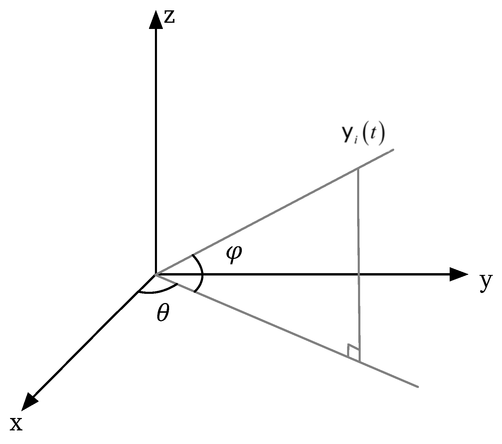
To estimate the angle, a MUSIC (Multiple Signal Classification) algorithm is adopted [17]. The algorithm model is shown in Figure 5. In Figure 5, $\varphi$ is the azimuth angle of arrival and $\theta$ is the zenith angle of arrival. ${\mathbf{y}}_i\left(t\right)$ is the time domain form of the received signal, corresponding to the frequency domain resource ${\mathbf{Y}}_i$.

The MUSIC algorithm is that the observation space of signal processing can be divided into signal subspace and noise subspace, and then the spatial–spectral function is constructed. The estimated angle of arrival direction corresponds to the angle of the peak at which the maximum of the spectral function is obtained in the spatial–spectral domain. $\Psi ({\widehat{\theta }}_i,{\widehat{\varphi }}_i)$ is expressed as

$$\Psi ({\widehat{\theta }}_i,{\widehat{\varphi }}_i)=\frac{1}{{{\mathbf{A}}_i}^{†}({\widehat{\theta }}_i,{\widehat{\varphi }}_i){\mathbf{V}}_i{{\mathbf{V}}_i}^{†}{\mathbf{A}}_i({\widehat{\theta }}_i,{\widehat{\varphi }}_i)}$$

(9)

where ${\mathbf{V}}_i$ is the noise matrix; ${\mathbf{A}}_i$ is the directional response vector with a normalized amplitude from ${\mathbf{H}}_i$. Calculation of ${\mathbf{A}}_i$ can be obtained by the eigenvalue decomposition of the received signal as follows

$$\begin{array}{cc}\hfill {\Re }_{\mathbf{Y}}& =\mathrm{E}\left\{{\mathbf{Y}}_i{\mathbf{Y}}_i^{†}\right\}\hfill \\ \hfill & ={\mathbf{H}}_i{\Re }_{\mathbf{r}}{{\mathbf{H}}_i}^{†}+{\widehat{\sigma }}^2\mathbf{I}\hfill \\ \hfill & ={\mathbf{U}}_i\wedge {\mathbf{U}}_i^{†}+{\widehat{\sigma }}^2{\mathbf{V}}_i{\mathbf{V}}_i^{†},\hfill \end{array}$$

(10)

where ${\Re }_{\mathbf{Y}}$ and ${\Re }_{\mathbf{r}}$ is the covariance matrix of received and transmitted SRS-Pos; ∧ is the eigenvalue matrix; ${\mathbf{U}}_i$ is an orthogonality matrix for signal;estimation of ${\widehat{\sigma }}^2$ can be reference to (7).

4.3. Joint Positioning Estimation

Assuming the coordinates of device and TRP positions are denoted as $\left(x_0,y_0,z_0\right)$ and $\mathcal{S}=\left\{\left(x_1,y_1,z_1\right),\dots ,\left(x_{N_{\mathrm{TRP}}},y_{N_{\mathrm{TRP}}},z_{N_{\mathrm{TRP}}}\right)\right\}$, the corresponding real distance and angle is $\mathcal{D}=\left\{d_1,\dots ,d_{N_{\mathrm{TRP}}}\right\}$ and $\Theta =\left\{({\theta }_1,{\varphi }_1),\dots ,({\theta }_{N_{\mathrm{TRP}}},{\varphi }_{N_{\mathrm{TRP}}})\right\}$, (8) and (9) can be re-expressed as

$$\begin{array}{c}\hfill \left\{\begin{array}{c}{\widehat{d}}_i=d_i+{\delta }_i\hfill \\ {\widehat{\theta }}_i={\theta }_i+{\delta }_i\hfill \\ {\widehat{\varphi }}_i={\varphi }_i+{\delta }_i\hfill \end{array}\right.\end{array},$$

(11)

where $d_i=\sqrt{{\left(x_0-x_i\right)}^2+{\left(y_0-y_i\right)}^2+{\left(z_0-z_i\right)}^2}$, ${\varphi }_i=arctan\left(\frac{z_0-z_i}{\left(x_0-x_i\right)cos{\widehat{\theta }}_i+\left(y_0-y_i\right)sin{\widehat{\theta }}_i}\right)$, ${\theta }_i=arctan\left(\frac{y_0-y_i}{x_0-x_i}\right)$, ${\delta }_i$ denotes the noise. Correspondingly, the estimated device position $\left({\widehat{x}}_0,{\widehat{y}}_0,{\widehat{z}}_0\right)$ can be obtained as

$$\begin{array}{c}\hfill \left\{\begin{array}{c}{\widehat{x}}_0=x_i+{\widehat{d}}_{i}cos{\widehat{\theta }}_i\hfill \\ {\widehat{y}}_0=y_i+{\widehat{d}}_{i}sin{\widehat{\theta }}_i\hfill \\ {\widehat{z}}_0=z_i+{\widehat{d}}_{i}sin{\widehat{\varphi }}_i\hfill \end{array}\right.\end{array}.$$

(12)

To solve (12) and obtain an accurate position of the target device, the estimated coordinates can be rewritten as

$$\left[\begin{array}{ccc}{\widehat{x}}_0& {\widehat{y}}_0& {\widehat{z}}_0\end{array}\right]=\mathbf{\Lambda }\left[\begin{array}{ccc}{\mathbf{\Gamma }}_x& {\mathbf{\Gamma }}_y& {\mathbf{\Gamma }}_z\end{array}\right],$$

(13)

where $\mathbf{\Lambda }$ is the optimization weight for positioning calculation, and ${\mathbf{\Gamma }}_x$, ${\mathbf{\Gamma }}_y$ and ${\mathbf{\Gamma }}_z$ can be expressed as

$$\left\{\begin{array}{c}{\mathbf{\Gamma }}_x={\left[x_1+{\widehat{d}}_{1}cos{\widehat{\theta }}_1,\dots ,x_{N_{\mathrm{TRP}}}+{\widehat{d}}_{N_{\mathrm{TRP}}}cos{\widehat{\theta }}_{N_{\mathrm{TRP}}}\right]}^T\hfill \\ {\mathbf{\Gamma }}_y={\left[y_1+{\widehat{d}}_{1}sin{\widehat{\theta }}_1,\dots ,y_{N_{\mathrm{TRP}}}+{\widehat{d}}_{N_{\mathrm{TRP}}}sin{\widehat{\theta }}_{N_{\mathrm{TRP}}}\right]}^T\hfill \\ {\mathbf{\Gamma }}_z={\left[z_1+{\widehat{d}}_{1}sin{\widehat{\varphi }}_1,\dots ,z_{N_{\mathrm{TRP}}}+{\widehat{d}}_{N_{\mathrm{TRP}}}sin{\widehat{\varphi }}_{N_{\mathrm{TRP}}}\right]}^T\hfill \end{array}\right.$$

(14)

4.4. Complexity Analysis

Based on the above description, it can be established that the main computation complexity is from IFFT operation, peak search and eigenvalue decomposition. For comparison, Let ${\Xi }_{\mathrm{TDOA}}$, ${\Xi }_{\mathrm{AoA}}$ and ${\Xi }_{\mathrm{joint}}$ be the signal processing complexity at each TRP under UL-TDOA, UL-AoA, and proposed joint UL-AoA+TDOA; the corresponding expression can be modeled as

$$\left\{\begin{array}{c}{\Xi }_{\mathrm{TDOA}}=\mathcal{O}\left(N_{\mathrm{R}}{N}_{\mathrm{FFT}}\right),\hfill \\ {\Xi }_{\mathrm{AoA}}=\mathcal{O}\left(N_{\mathrm{R}}{N}_{\mathrm{FFT}}\right)+\mathcal{O}\left(N_{\mathrm{R}}^3\right)+\mathcal{O}\left(N_{\theta }{N}_{\phi }\right),\hfill \\ {\Xi }_{\mathrm{joint}}=\mathcal{O}\left(2N_{\mathrm{R}}{N}_{\mathrm{FFT}}\right)+\mathcal{O}\left(N_{\mathrm{R}}^3\right)+\mathcal{O}\left(N_{\theta }{N}_{\phi }\right),\hfill \end{array}\right.$$

(15)

where $N_{\theta }$ and $N_{\phi }$ is the quantitative space of each ${\theta }_i$ and ${\phi }_i$. As shown in Figure 5, ${\theta }_i$ ranges over $\left\{-\pi ,\pi \right\}$, and ${\phi }_i$ is within $\left\{-\pi /\phantom{\pi 2}2,\pi /\phantom{\pi 2}2\right\}$. It should be noted that a common complexity introduced by $N_{\mathrm{symb}}^{\mathrm{SRS}}{N}_{\mathrm{RE}}^{\mathrm{SRS}}$ is ignored in the above expression, since the basic signal processing is required under each algorithm. In Section 5.2, we also quantified the time complexity.

5. Simulation Results

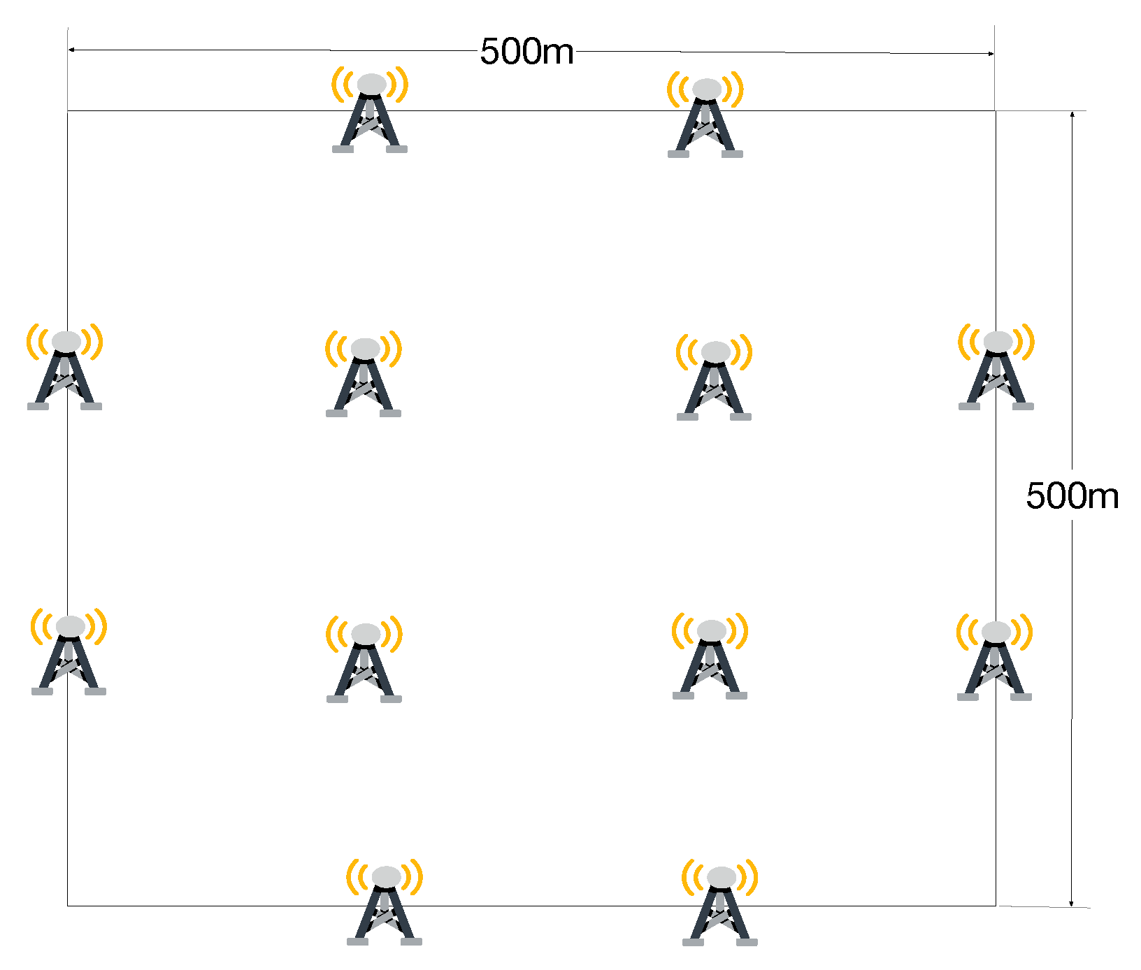
Unless specified otherwise, the simulation setting is given in

Table 3. Simulation setting.

Parameter	Value
Simulation environment	Indoor, 500 m × 500 m
Total TRP number	12
TRP number for localization	3
Network duplex mode	TDD
Frequency range	27–28 GHz
System bandwidth	400 MHz
Subcarrier spacing	120 KHz
SNR	22 dB
$N_{\mathrm{R}}$	64
$K_{\mathrm{TC}}^{\mathrm{SRS}}$	2
$N_{\mathrm{symb}}^{\mathrm{SRS}}$	1
$N_{\mathrm{PRB}}^{\mathrm{SRS}}$	272
$N_{\mathrm{FFT}}$	4096

. Take an indoor square factory with 500 m × 500 m [1], in which devices are uniformly distributed. There are 12 TRPs within the factory, and 3 TRPs perform the measurement for a target device by default. The network is a TDD system operating in 27-28GHz with a subcarrier spacing as 120 KHz and a 400 MHz bandwidth. The simulation scenario is shown in Figure 6.

5.1. Performance of SRS-Pos under Different Configuration

Positioning accuracy depends on the measurement results, such as timing delay and angle, which is impacted by the transmission environment denoted as SNR. Therefore, we should evaluate the detection accuracy vs. SNR. The detection accuracy is computed by (16)

$$\left\{\begin{array}{c}Angleestimationerrorrate=\frac{1}{N}{\displaystyle \sum _{n=1}^N}\mathrm{Y}(\left|estimatedangl{e}_n-trueanglevalue\right|>anglethreshold),\hfill \\ \\ Timeestimationerrorrate=\frac{1}{N}{\displaystyle \sum _{n=1}^N}\mathrm{Y}(\left|estimatedtim{e}_n-truetimevalue\right|>timethreshold)\hfill \end{array}\right.$$

(16)

where N is the total simulation time, $\mathrm{Y}\left(x\right)$ is a function as

$$\mathrm{Y}\left(x\right)=\left\{\begin{array}{ccc}\hfill 1& & ifxisture\hfill \\ \hfill 0& & ifxisfalse\hfill \end{array}\right.$$

and represents whether the estimate is wrong. The angle threshold is set to the range of plus or minus two degrees of the true angle value, and the time threshold is set to the range of plus or minus 4 ns of the true time value. Once the estimated result exceeds that range, it is considered that the estimation is wrong and x is true. So the value of $\mathrm{Y}\left(x\right)$ is one. After completing N times of estimation, the proportion of the times of wrong estimation to the total estimation times is calculated, as in (16), and the value of Angle estimation error rate or Time estimation error rate is obtained. Considering the detection error due to the randomization of the transmission environment, the average operation is performed.

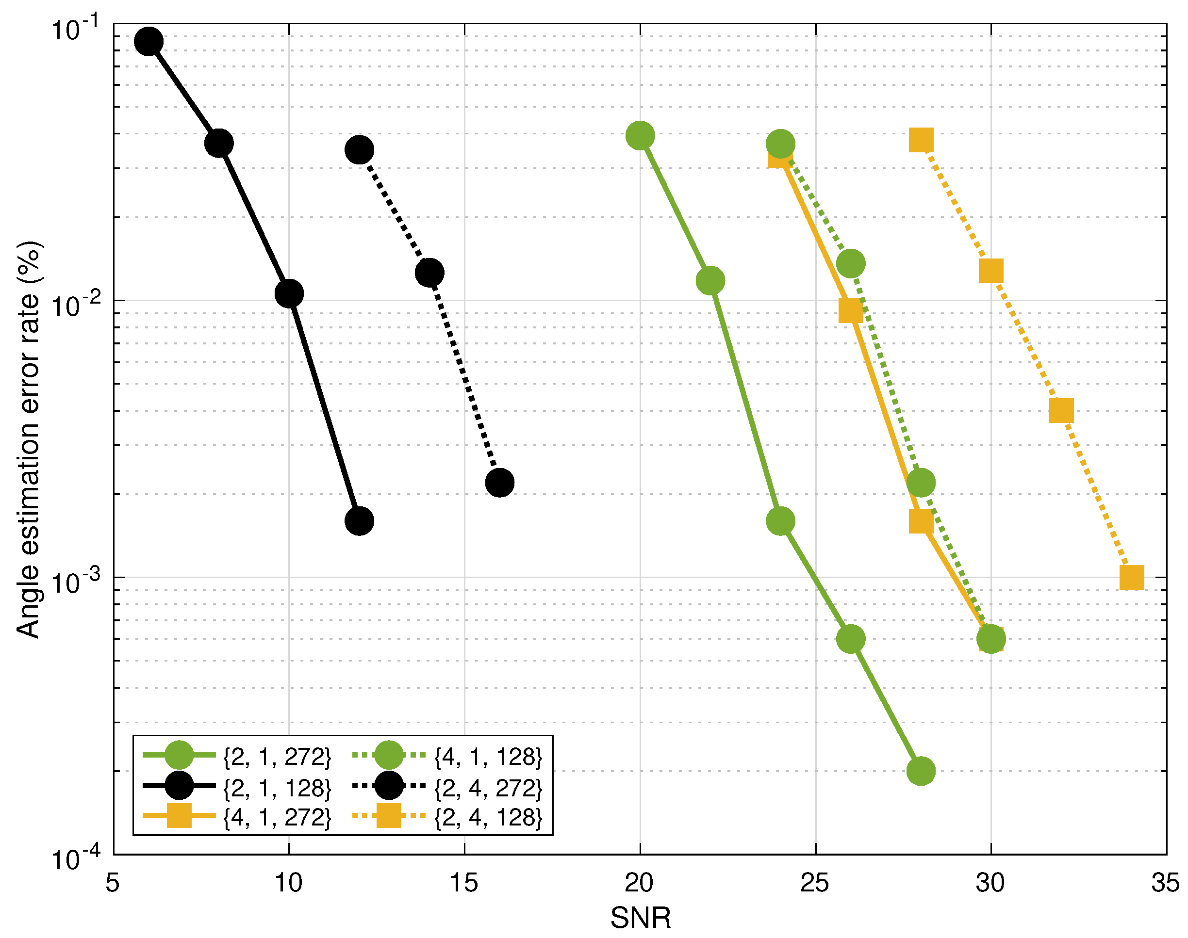
Figure 7 shows angle estimation error of SRS-Pos with a combination configuration $\left\{K_{\mathrm{TC}}^{\mathrm{SRS}},N_{\mathrm{symb}}^{\mathrm{SRS}},N_{\mathrm{PRB}}^{\mathrm{SRS}}\right\}$. In Figure 7, the ordinate represents the angle estimation error, and it is calculated by i (16). The full line and the dotted line compares the results under a maximum SRS-Pos bandwidth, i.e., $N_{\mathrm{PRB}}^{\mathrm{SRS}}=272$ and $N_{\mathrm{PRB}}^{\mathrm{SRS}}=128$, respectively. Obviously, it can be observed that the performance is enhanced with the increase in bandwidth. The square marker and the circle marker denotes the result under $N_{\mathrm{symb}}^{\mathrm{SRS}}=4$ and $N_{\mathrm{symb}}^{\mathrm{SRS}}=1$ OFDM symbol in time domain. With the same configuration of bandwidth and comb size, the accuracy is improved with the increase in $N_{\mathrm{symb}}^{\mathrm{SRS}}$, since the cumulated power increases with $N_{\mathrm{symb}}^{\mathrm{SRS}}$.

Further, it can be observed from Figure 7 that the accuracy is always better under a smaller $K_{\mathrm{TC}}^{\mathrm{SRS}}$, since the valid sequence length is inversely proportional with $K_{\mathrm{TC}}^{\mathrm{SRS}}$. Fortunately, the performance degradation of larger comb size can be compensated by the time domain duration. As illustrated, $\left\{4,1,272\right\}$ and $\left\{2,1,128\right\}$ have a similar performance. Though there is 3 dB degradation under $K_{\mathrm{TC}}^{\mathrm{SRS}}=4$, the bandwidth size is around two times that of the $\left\{2,1,128\right\}$ case. The SRS-Pos sequence lengths under $\left\{4,1,272\right\}$ and $\left\{2,1,128\right\}$ are 816 and 768, respectively.

Figure 8 shows a time estimation error of SRS-Pos with a combination configuration $\left\{K_{\mathrm{TC}}^{\mathrm{SRS}},N_{\mathrm{symb}}^{\mathrm{SRS}},N_{\mathrm{PRB}}^{\mathrm{SRS}}\right\}$. In this figure, the ordinate represents the time estimation error, and it is calculated by i (16). Two different colors represents two different comb sizes. It can be observed that the estimation accuracy under $K_{\mathrm{TC}}^{\mathrm{SRS}}=2$ outperforms that of $K_{\mathrm{TC}}^{\mathrm{SRS}}=4$. Especially, for $\left\{2,2,28\right\}$ and $\left\{4,4,28\right\}$, the performance of the former is around 1.5 dB better, while the SRS-Pos length of the former is twice of the latter and the duration of former is half of the latter. This can prove that the sequence autocorrelation and crosscorrelation plays an more important role for sequence detection than the power cumulation in the time domain. However, under the same comb size configuration, the estimation error decreases with the sequence time domain duration $N_{\mathrm{symb}}^{\mathrm{SRS}}$.

5.2. Positioning Accuracy

For performance comparison, TDOA-only, AoA-only and joint TDOA + AoA are tested. As depicted in Figure 9, the performance of the joint positioning method outperforms that of TDOA only and AoA only under lower SNR (smaller than 22 dB) and the performance gap is around 17%, while the performance gap diminishes gradually with the increase in SNR (larger than 22 dB). It is reasonable that sequence detection is better in case of good radio link environment. In this figure, it can be found that TDOA only and AoA only have similar positioning accuracy. However, it should be noted that the measurement load is larger under TDOA only, since at least three TRPs are required to localize a target device exactly.

Table 4. Simulation setting.

Parameter	Running Time
TDOA-only	0.5856 s
AoA-only	3.0083 s
joint TDOA + AoA	3.5624 s

shows the running time required by TDOA only, AoA only and Joint TDOA + AoA to complete a UE positioning.

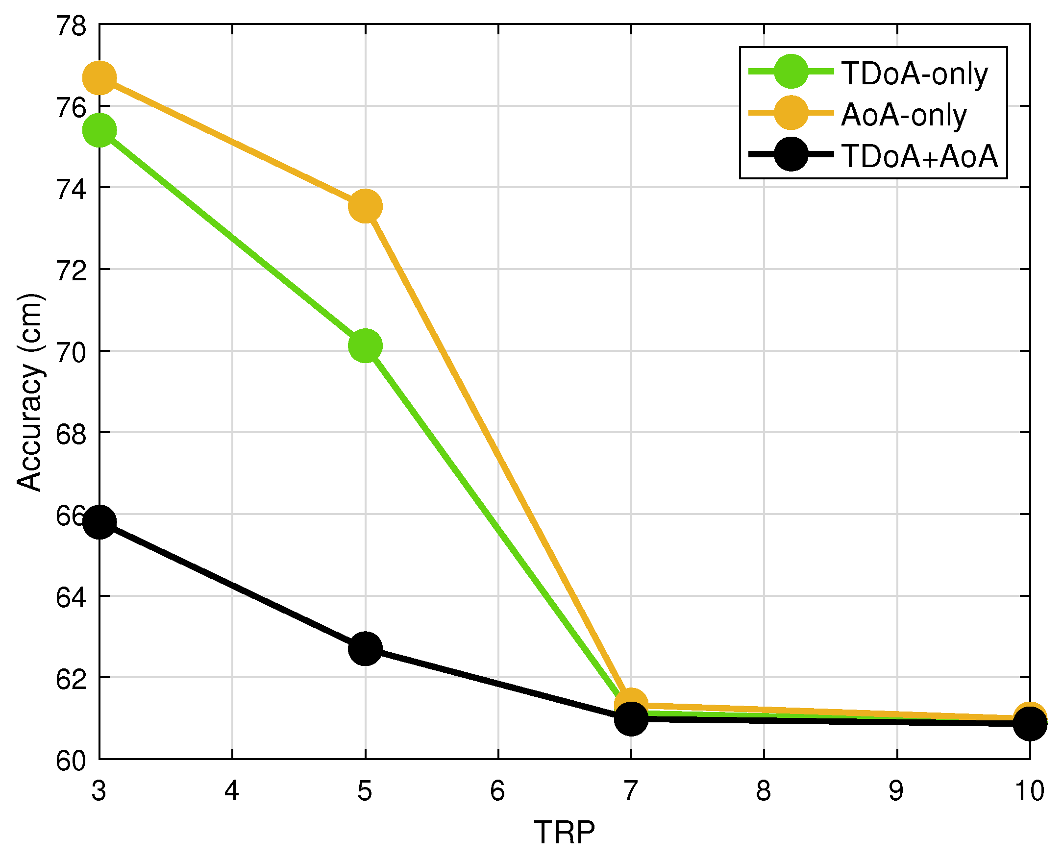
Moreover, the performance impact of TRP number on the positioning accuracy is illustrated in Figure 10 with a working SNR as 22 dB. There is no doubt that better positioning accuracy can be obtained under the joint positioning method, and the accuracy can be improved by around 13%. With the increase in TRP numbers, the performance gap decreases. While the TRP number is larger than seven, there is basically no difference between the three methods.

One thing to declare is the accuracy is obtained by a 1% error estimation of delay and angle, i.e., working SNR, is 22 dB, as shown in Table 3. It can be found that the accuracy is limited to around 60 cm. The main reason is the system setting of 120 KHz and frequency range restricts the positioning accuracy, as shown in (8). Until now, the testing or simulation for 5G positioning has been quite different, and this paper compares the performance with results in [15] wherein the localization is based on time estimation measurement. It could be found that the joint positioning method can improve the localization accuracy to submeter around 27 GHz. However, it should be also noted that the performance enhancement is at the cost of increased computation complexity. According to (15) with $N_{\theta }=360$ and $N_{\phi }=180$ corresponding to a $1^{\circ }$ angle searching granularity, and system parameters in Table 3, the processing complexity under the joint positioning is around 3.2× and 1.4× of that under the TDOA only and AoA only. According to the positioning accuracy specification in [1,10], the requirement is down to 10–20 cm for indoor positioning. Therefore, we think the complexity is worth the increased accuracy.

6. Conclusions

In this paper, we have investigated the positioning method for IIoT with a mm-Wave communication. The design of PRS and SRS-Pos are fully discussed to provide the problem model. Under the real constrict of power limitation and IoT packet size, a joint UL time and angle estimation method is analyzed. By giving the general system model, the time and angle estimation are derived for positioning, respectively. Through combining the time and angle together, the localization of an IIoT device is improved according to the simulation results.

In future work, regarding the joint DL and UL positioning, we will further investigate the impact of the device number on the positioning method, since the measurement load at TRPs increases with the device number. Especially, in case of massive machine type communication (mMTC) with a density of 1 connection/${\mathrm{m}}^2$, it is a huge burden for TRPs to perform positioning.

References

- 3GPP, TS 22.261 V18.6.0, Service Requirements for the 5G System (Release 18). December 2022. Available online: https://portal.3gpp.org/ChangeRequests.aspx?q=1&specnumber=22.261 (accessed on 14 June 2021).
- 3GPP, TR 38.825 V16.0.0, Study on NR Industrial internet of Things (IoT) (Release 16). April 2019. Available online: https://portal.3gpp.org/ChangeRequests.aspx?q=1&specnumber=38.825 (accessed on 9 October 2021).
- 3GPP, TR 22.872 V16.1.0, Study on Positioning Use Cases (Release 16). August 2018. Available online: https://portal.3gpp.org/ChangeRequests.aspx?q=1&specnumber=22.872 (accessed on 17 February 2022).
- Ghosh, A.; Ratasuk, R.; Rao, A.M. Industrial IoT Networks Powered by 5G New Radio. Microw. J. 2019, 62, 24–40. [Google Scholar]
- Dardari, D.; Closas, P.; Djuric, P.M. Indoor Tracking: Theory, Methods, and Technologies. IEEE Trans. Veh. Technol. 2015, 64, 1263–1278. [Google Scholar] [CrossRef] [Green Version]
- Peral-Rosado, J.D.; Raulefs, R.; Lopez-Salcedo, J.A.; Seco-Granados, G. Survey of Cellular Mobile Radio Localization Methods: From 1G to 5G. IEEE Commun. Surv. Tutorials 2018, 20, 1124–1148. [Google Scholar] [CrossRef]
- Phelan. Smart Manufacturing & the IoT-Enabled Smart Factory. Available online: https://www.inpixon.com/blog/smart-manufacturing-iot-enabled-smart-factory (accessed on 4 March 2022).
- 3GPP, TR 38.855, V16.0.0, Study on NR Positioning Support (Release 16). March 2019. Available online: https://portal.3gpp.org/desktopmodules/Specifications/SpecificationDetails.aspx?specificationId=3501 (accessed on 27 September 2021).
- 3GPP. Low Power High Accuracy Positioning for Industrial Iot Scenarios. 3GPP Work Item Description, S1-210365. Available online: https://www.3gpp.org/ftp/tsg_sa/WG1_Serv/TSGS1_93e_Electronic_Meeting/Docs/S1-210365.zip (accessed on 17 February 2022).
- 3GPP, TS 22.104 V18.0.0, Service Requirements for the Cyber-Physical Control Applications in Vertical Domains (Release 18). April 2021. Available online: https://portal.3gpp.org/ChangeRequests.aspx?q=1&specnumber=22.104 (accessed on 23 February 2022).
- 3GPP, TS 38.305, NG Radio Access Network (NG-RAN); Stage 2 Functional Specification of User Equipment (UE) Positioning in NG-RAN, 2020. Available online: https://portal.3gpp.org/ChangeRequests.aspx?q=1&specnumber=38.305 (accessed on 3 August 2021).
- Liang, M.; Li, X.H.; Zhang, W.G.; Liu, D.Z. The Generalized Cross-Correlation Method for Time Delay Estimation of Infrasound Signal. In Proceedings of the 2015 Fifth International Conference on Instrumentation and Measurement, Computer, Communication and Control (IMCCC), Qinhuangdao, China, 18–20 September 2015; pp. 1320–1323. [Google Scholar]
- Yizhou, H.E.; Cui, G.; Pengxu, L.I.; Chang, R.; Wang, W. Timing advanced estimation algorithm of low complexity based on DFT spectrum analysis for satellite system. China Commun. 2015, 12, 140–150. [Google Scholar] [CrossRef]
- 3GPP, TS 38.211 V16. 0. 0, NR: Physical Channels and Modulation (Release 16). December 2019. Available online: https://portal.3gpp.org/ChangeRequests.aspx?q=1&specnumber=38.211 (accessed on 9 June 2021).
- Yi, L.; Richter, P.; Lohan, E.S. Opportunities and challenges in the industrial internet of things based on 5G positioning. In Proceedings of the 2018 8th International Conference on Localization and GNSS (ICL—GNSS), Guimaraes, Portugal, 26–28 June 2018. [Google Scholar]
- Zhou, B.; An, L.; Lau, V. Successive Localization and Beamforming in 5G mmWave MIMO Communication Systems. IEEE Trans. Signal Process. 2019, 67, 1620–1635. [Google Scholar] [CrossRef]
- Schmidt, R. Multiple emitter location and signal parameter estimation. IEEE Trans. Antennas Propag. 1986, 34, 276–280. [Google Scholar] [CrossRef] [Green Version]
- Wang, Y.; Ho, K.C. Unified Near-Field and Far-Field Localization for AOA and Hybrid AOA-TDOA Positionings. IEEE Trans. Wirel. Commun. 2018, 17, 1242–1254. [Google Scholar] [CrossRef]
- Wang, Y.; Ho, K.C. An Asymptotically Efficient Estimator in Closed-Form for 3-D AOA Localization Using a Sensor Network. IEEE Trans. Wirel. Commun. 2015, 14, 6524–6535. [Google Scholar] [CrossRef]
- Zhao, Y.; Qi, W.; Liu, P.; Chen, L.; Lin, J. Accurate 3D localisation of mobile target using single station with AoA/TDoA measurements. IET Radar Sonar Navig. 2020, 14, 954–965. [Google Scholar] [CrossRef]
- Ketabalian, H.; Biguesh, M.; Sheikhi, A. A Closed-Form Solution for Localization Based on RSS. IEEE Trans. Aerosp. Electron. Syst. 2020, 56, 912–923. [Google Scholar] [CrossRef]
- Chen, T.; Wang, M.; Huang, X.; Xie, Q. TDOA-AoA Localization Based on Improved Salp Swarm Algorithm. In Proceedings of the 2018 14th IEEE International Conference on Signal Processing (ICSP), Beijing, China, 12–14 August 2018; pp. 108–112. [Google Scholar]
- Yue, Y.; Cao, L.; Hu, J.; Cai, S.; Hang, B.; Wu, H. A Novel Hybrid Location Algorithm Based on Chaotic Particle Swarm Optimization for Mobile Position Estimation. IEEE Access 2019, 7, 58541–58552. [Google Scholar] [CrossRef]
- Kanhere, T.; Rappaport, S. Position Locationing for Millimeter Wave Systems. In Proceedings of the 2018 IEEE Global Communications Conference (GLOBECOM), Abu Dhabi, United Arab Emirates, 9–13 December 2018; pp. 206–212. [Google Scholar]
- Thakur, N.; Han, C.Y. Multimodal approaches for indoor localization for ambient assisted living in smart homes. Information 2021, 12, 114. [Google Scholar] [CrossRef]
- Posluk, M.; Ahlander, J.; Shrestha, D.; Modarres Razavi, S.; Lindmark, G.; Gunnarsson, F. 5G Deployment Strategies for High Positioning Accuracy in Indoor Environments. arXiv 2021, arXiv:2105.09584. [Google Scholar]
- Tsiropoulou, E.E.; Paruchuri, S.T.; Baras, J.S. Interest, energy and physical-aware coalition formation and resource allocation in smart IoT applications. In Proceedings of the 2017 51st Annual Conference on Information Sciences and Systems (CISS), Baltimore, MD, USA, 22–24 March 2017; pp. 1–6. [Google Scholar]
- Wang, Y.; Li, C.; Yu, Y.; Huang, S. Enabling Low-Power High-Accuracy Positioning (LPHAP) in 3GPP NR Standards. In Proceedings of the 2021 International Conference on Indoor Positioning and Indoor Navigation (IPIN), Lloret de Mar, Spain, 29 November–2 December 2021; pp. 1–7. [Google Scholar]
- 3GPP, TS 36.355 V.16.0.0, Evolved Universal Terrestrial Radio Access (E-UTRA); LTE Positioning Protocol (LPP) (Release 16). July 2014. Available online: https://portal.3gpp.org/ChangeRequests.aspx?q=1&specnumber=36.355 (accessed on 9 June 2021).
- Zhang, Y. Improvements on Otdoa and Agnss Positioning and Timing Information Obtaining and Updating, WO, WO2011100859 A8. Available online: https://patents.google.com/patent/WO2011100859A1/un (accessed on 22 June 2021).
Figure 1.
Illustration of PRS and SRS-Pos design architecture. (a) PRS Design architecture, (b) SRS-Pos design architecture.
Figure 2.
Illustration of PRS and SRS-Pos comb-based time-frequency RE mapping. (a) PRS comb-based RE mapping. (b) SRS-Pos comb-based RE mapping.
Figure 3.
Illustration of PRS and SRS-Pos comb-based time-frequency RE mapping. (a) no muting. (b) muting opt1. (c) muting opt2. (d) muting opt1+opt2.
Figure 4.
Signal Processing flow of joint UL-AoA and UL-TDOA positioning.
Figure 5.
Signal arrival direction model.
Figure 6.
Simulation scenario of indoor square factory.
Figure 7.
Illustration of angle estimation error with SRS-Pos configuration .
Figure 8.
Illustration of timing estimation error with SRS-Pos configuration .
Figure 9.
Illustration of positioning accuracy vs. SNR.
Figure 10.
Illustration of positioning accuracy vs. TRP number.