Improve Stock Price Model-Based Stochastic Pantograph Differential Equation

Abstract

Although the concept of symmetry is widely used in many fields, it is almost not discussed in finance. This concept appears to be relevant in relation, for example, to mathematical models that can predict stock prices to contribute to the decision-making process. This work considers the stock price of European options with a new class of the non-constant delay model. The stochastic pantograph differential equation (SPDE) with a variable delay is provided in order to overcome the weaknesses of using stochastic models with constant delay. The proposed model is constructed to improve the evaluation process and prediction accuracy for stock prices. The feasibility of the proposed model is introduced under relatively weak conditions imposed on its volatility function. Furthermore, the sensitivity of time lag is discussed. The robust stochastic theta Milstein (STM) method is combined with the Monte Carlo simulation to compute asset prices within the proposed model. In addition, we prove that the numerical solution can preserve the non-negativity of the solution of the model. Numerical experiments using real financial data indicate that there is an increasing possibility of prediction accuracy for the proposed model with a variable delay compared to non-linear models with constant delay and the classical Black and Scholes model.

1. Introduction

Stochastic Differential Equation (SDE) has been used for modeling the asset price for different types of option price valuations. The Black–Scholes (BS) formula is considered the most important model in terms of application in the study of continuous-time financial models based on a SDE [1]. The motivation of the BS model of normality of the returns distribution and constant volatility was criticized in [2] because empirical studies provided that volatility actually depends on time in a way that is not predictable. That observation led to the construction of dynamic models based on non-constant volatility in order to improve the understanding of the behavior of natural processes.

Recently, the Stochastic Functional Differential Equation (SFDE) has received increased interest in many simulated dynamical systems based on some kind of past dependence. Hobson and Rogers [3] provided a new non-constant volatility model with past dependency in finance. Arriojas et al. [4] assumed that the stock price satisfies an SFDE with fixed or variable delays. For Mao and Sabanis [5], it seems natural to consider this approach where volatility can be regarded as a function of past events. In addition, the pricing of European options on two underlying assets with delays is discussed in [6]. For reasons of notational simplicity and elegance, previous work assumed that the stock price follows a special form of SFDE; a Stochastic Delay Differential Equation (SDDE) with a constant delay time. The motivation for introducing SDDE is the estimation of the volatility function $g(V(t-\tau ))$ based on a constant delay time $t-\tau$. However, Liu [7] provided the weaknesses of the SDDE with a constant delay time as: (1) The memory (past event) cannot be considered in $t<\tau$; (2) The constant delay τ is only suitable for short period memory (bounded memory).

The main question of this work is, is there another form of SFDE support that uses the memory effect (past dependence) as a real-time variable function that can overcome the weaknesses of SDDE in addition to increasing the prediction accuracy?

The aim of this paper is to consider another kind of SFDE with avariable delay [8,9,10]. The Stochastic Pantograph Differential Equation (SPDE) for modeling stock prices will be obeyed. SPDE is a special type of past-dependence equation with many special properties such as unbounded memory and a variable delay time $(t-qt)$, which is namely the pantograph delay and can be written as $(qt)$. SDDE is the motivation for introducing a new class of stock price-SPDE (SP-SPDE) models with non-constant volatility; it is the estimation of volatility function based on the pantograph delay in order to overcome the weaknesses of SDDE and increase the prediction accuracy. The proposed SP-SPDE model that has a unique non-negative solution under relatively weak conditions imposed on its volatility function will be shown (i.e., the SP-SPDE model is feasible for evaluating the underlying stock price).

Due to using financial models based on the past dependence, it can be observed that there is a time lag, q, in the SP-SPDE model. In this work, it is proven that the small changes in the time lag q of the SP-SPDE model have an analogously small impact on the values of the stock price. The robustness of the delay effect on stock price valuation is shown (i.e., the variable delay effect is not too sensitive to time lag changes).

Preserving non-negativity approximate solutions for stochastic models that meet positivity solutions has received increased interest in recent times for use in financial mathematics. Although Kahl [11] shows the different ways to avert the numerical negativity, the balanced implicit method (BIM) method and the Milstein method have proven that the numerical method based on the Euler scheme is a finite time for all SDE (i.e., the numerical methods do not preserve positivity of the solution of SDEs), recently published research still considers numerical methods based on the Euler scheme in order to approximate the paths of stochastic models with respect to delay dependence in financial mathematics [5,12]. Based on Kahl’s work, there are few works in the literature discussing this issue; for example, the fundamental analysis of Milstein-type methods with respect to non-negativity has been discussed for a family of financial models [13,14,15,16,17,18,19]. Moreover, classes of the BIM method were provided in [20,21,22]. Here, note that Kahl said, “the Milstein method has two advantages in comparison with the BIM. On the one hand, the convergence rate is twice as high as in the BIM and, on the other hand, positivity can be achieved without using control functions”. In addition, there are are few studies discussing the Milstein-type schemes for SPDE without considering the issue of the positivity of numerical solutions [23]. Therefore, this paper will consider the stochastic theta Milstein (STM) method to numerically solve the SP-SPDE model using real data. This paper will prove that the STM scheme can preserve the positivity of the solution for a family of financial models based on SPDE, using real data. The comparison will be performed for the proposed non-linear variable-delayed SP-SPDE model with a constant delay SDDE model in [5] and the classical Black–Scholes model [1]. To the best of our knowledge, such a comparison between variable and constant delay models has not yet been performed in the financial literature.

The paper is organized as follows. In Section 2, the non-linear variable delay SP-SPDE model for stock prices is provided. Furthermore, the paper shows how SPDE can overcome the weaknesses of SDDE related to financial quantity. In Section 3, the paper proves how the proposed model is feasible for evaluating the underlying stock price. The time-lag sensitivity of the proposed model is discussed in Section 4. Section 5 proposes the numerical STM method for the SP-SPDE model, and the non-negativity of the solution is discussed. Numerical experiments for the variable delay model, constant delay model and classical Black–Scholes model using real data for some firms in order to show the prediction accuracy of the proposed model is shown in Section 6. The conclusion is provided in Section 8.

2. Stock Price Model with a Variable Delay

A complete probability space is defined as $(\mathsf{\Omega },\mathcal{F},{\{{\mathcal{F}}_t\}}_{t\ge 0},P)$ with a filtration ${\{{\mathcal{F}}_t\}}_{t\ge 0}$, which satisfies the usual conditions, i.e., the filtration ${\{{\mathcal{F}}_t\}}_{t\ge 0}$ is right-continuous and each $\{{\mathcal{F}}_t\},t\ge 0$ contains all $\mathbb{P}$-null sets. Let $W(t)$, $t\ge 0$ be ${\mathcal{F}}_t$-adapted and independent of ${\mathcal{F}}_0$, be a scalar Brownian motion defined on the above probability space. $|·|$ is the Euclidean norm in $\mathbb{R}$. Let $x_0$ be ${\mathcal{F}}_0$-measurable and $E|x_0{|}^2\le M<+\infty$. Moreover, ${\mathbb{R}}_{+}=[0,+\infty )$ and $C({\mathbb{R}}_{+};{\mathbb{R}}_{+})$ denote the space of all non-negative continuous functions defined on ${\mathbb{R}}_{+}$.

In the literature of financial mathematics, the Black–Scholes in [1] assumes that the value of the stock price at time $t\in [0,T],S(t)$ follows an SDE as follows

$$\mathrm{d}S(t)=rS(t)\mathrm{d}(t)+\sigma S(t)\mathrm{d}W(t),$$

(1)

where $S(0)$ is given, $r>0$ is the risk-free interest rate, and $\sigma$ is the constant volatility of the stock return per unit of time with one-dimensional standard Brownian motion process W.

In order to improve the understanding of the behavior of natural processes and overcome the disadvantages of the classic Black–Scholes model (1), such as the normality of the returns distribution and constant volatility, the new dynamic model has been provided based on considering non-constant volatility and past dependency on the current and future states of the stock price, which follows an SDDE with a constant delay time in [4,5,6]. They assumed that a stock price $S(t)$ follows an SDDE with constant delay time as

$$\mathrm{d}S(t)=r(S(t-\tau ))S(t)\mathrm{d}(t)+g(S(t-\tau ))S(t)\mathrm{d}W(t),$$

(2)

with initial data $S(u)=\xi (u)$ on $u\in [-\tau ,0]$. The positive constant $\tau$ represents the past length while T is the maturity date. The motivation for introducing SDDE is the estimation of the volatility function $g(S(t-\tau ))$ based on a constant delay time $t-\tau$. However, Liu [7] provided the weaknesses of choice of the SDDE with a constant delay time as; (1) The memory (past event) cannot be considered in $t<\tau$. (2) The constant delay τ is only suitable for short period memory (bounded memory).

In the following, another form of a dynamic model based on the memory effect (past dependence) as a real-time variable function that can overcome the weaknesses of SDDE in addition to the possibility of increasing the prediction accuracy is provided. In general, a memory effect (influence past event) can be given in terms of delay function $h(t)$ such that the value at the current time t depends on the knowledge of the past (delay) time $t-h(t)$. For simplicity, a routine way is to take a delay function $h(t)=\tau ,\tau >0$, which leads to a constant delay time $(t-\tau )$ in the SDDE model (2). In order to overcome the weaknesses of the constant delay, the delay function $h(t)=\delta t$ with $0<\delta <1$ is chosen, hence the delay time will be $t-h(t)$=$(1-\delta )t=qt$, where $q=1-\delta$ and $q\in (0,1)$. This treatment leads to a variable delay (pantograph delay), which is the main motivation of SPDE. It seems natural to consider an approach where volatility can be regarded as a function of the variable’s past states $S(qt)$. It is assumed that the stock price process $S(t)$ at time $t\in [0,T]$ can be governed by the following SPDE, which will be called the SP-SPDE model in this work.

$$\mathrm{d}S(t)=r(S(qt))S(t)\mathrm{d}(t)+g(S(qt))S(t)\mathrm{d}W(t),$$

(3)

with initial values $S(0)=S_0$ and $q\in (0,1)$. $r>0$ is the risk-free interest rate, and $W(t)$ is the scalar Brownian motion. $g:\mathbb{R}\to \mathbb{R}$ is the volatility function.

In the beginning, in order to explain how SPDE can overcome the weaknesses of SDDE in terms of financial quantity, the following example is provided.

Example 1.

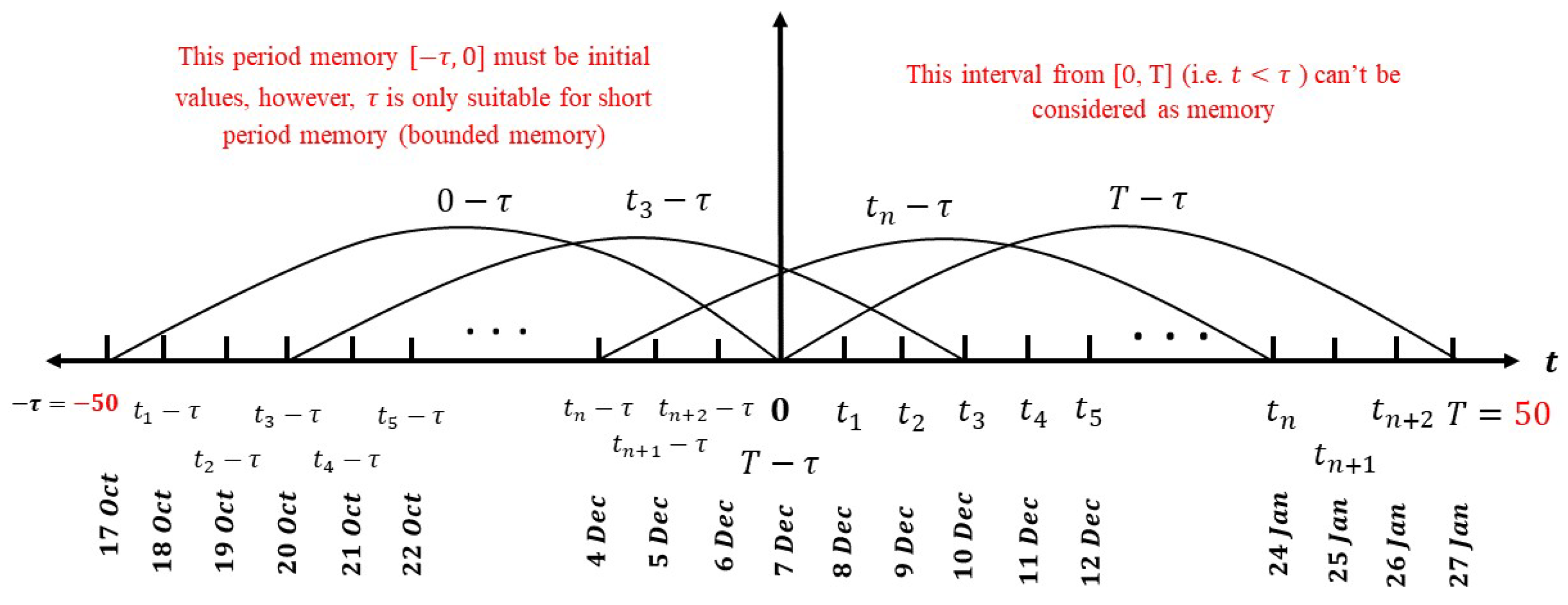
Lin et al. [6] considered stock price values whose value depends on the stock price and time using an SDDE (2). On application with real data of Aaron’s. Inc. (AAN.N) from 17 October 2005 to 27 January 2006 (i.e., about 100 days), they assume that $T=\tau =50$, the data between [17 October 2005 to 7 December 2005] are used as memory data (i.e., $[-\tau ,0]\simeq [-50,0]$), while those between [7 December 2005 and 27 January 2006] are used as the future data (i.e., $[0,T]\simeq [0,50]$) for the models to predict.

We can explain the deficiencies in the use of the SDDE model (2) as follows (see Figure 1).

• The past event cannot be considered in the interval of the future (predictable) data $[0,T]$ [7 December 2005 to 27 January 2006] since the past event $S(t-\tau )\in [-\tau ,0]$ (i.e., the memory (past event) cannot be considered in $[0,T]$ or $t<\tau$),
• There is no empirical evidence to explain the correlation between the current stock price at t and its past price at $t-\tau$ and how to determine the value of time lag $\tau$ (i.e., what is the correlation between the stock price today and its price 50 days ago when considering $\tau =50$),
• The data in the memory interval $[-\tau ,0]$ [17 October 2005 to 7 December 2005] must be available because the value $S(t-\tau )\in [-\tau ,0]$ is wanted for simulating the model (i.e., the constant delay $\tau$ is only suitable for short period memory (bounded memory) with a restriction of the need for historical data during the period $[-\tau ,0]$).

In the following points, we can see the advantage of choosing a variable delay in SPDE vs. the weaknesses of a constant delay in SDDE (See Figure 2).

• The past event can be considered in the interval of the future (predictable) data $[0,T]$ [7 December 2005 to 27 January 2006] since the past event $S(qt)\in [0,T]$. Based on $q\in (0,1)$, most of the interval $[0,T]$ [7 December 2005 to 27 January 2006] can be considered as memory; let $q=0.2,0.5,0.7$ or $0.9$, then $20\%,50\%,70\%$ or $90\%$ of this data can be considered as memory (i.e., this property can overcome the weakness of SDDE as “The memory (past event) cant be considered in $t<\tau$.”).
• It makes more sense to consider that the data in the recent past are more effective in determining the stock price at the current and future events. This idea can be considered by choosing the value of time lag q to control the correlation between the past events and the current and future events in sight of the properties of a pantograph delay time $qt$.
• Based on the feature of the initial value $S(0)=S_0$ and past delay time $qt$, the SPDE has special properties such that it is suitable for long period memory (unbounded memory) (i.e., this property can overcome the weakness of SDDE as “The constant delay $\tau$ is only suitable for short period memory (bounded memory))”.

However, one of the motivations of this work is the estimation of the volatility function $g(V(qt))$ based on the variable past dependence $qt$ (pantograph delay). Following [4,5,12,24], the form of volatility functions that would be more suitable for the proposed model will not be discussed because a lot of previous work on that point has made it clear that the conditions imposed on it are very weak, so a wide class of volatility functions may be used to fit a wide range of financial quantities. In the next sections we will prove the feasibility of the proposed non-constant non-linear stochastic variable delay model (SP-SPDE) for simulating the stock price.

3. Feasibility of the SP-SPDE Model for Stock Price

The feasibility of the financial model is one of the most important characteristics to be demonstrated in the sense that they admit pathwise unique positive solutions such that $S(t)>0$, almost surely $\forall t\ge 0$ whenever the initial path $S(0)>0$. In this section, the feasibility of the proposed SP-SPDE model for simulating the stock price will be proven, which can be considered as

$$\mathrm{d}S(t)=rS(t)\mathrm{d}(t)+g(S(qt))S(t)\mathrm{d}W(t),$$

(4)

In order to guarantee that the SP-SPDE model (4) has a unique global positive solution, it is assumed that the volatility function g is bounded and satisfies the local Lipschitz condition (see [10]). The following theorem proves that the model is feasible in the sense that they admit a pathwise unique solution that $S(t)>0$ almost surely for $t\in [0,T]$, with initial conditions $S(0)>0$ and $g(S(qt))\ne 0$∀$S(qt)\in \mathbb{R}$.

Theorem 1.

The stock price model (4) has a pathwise unique global positive solution $S(t)>0$ for a given initial value $S(0)>0\forall t\ge 0$, which can be computed step by step as follows

$$S(t)=S(0)exp\left\{rt-\frac{1}{2}{\int }_0^t{g}^2(S(qu))\mathrm{d}(u)+{\int }_0^{t}g(V(qu))\mathrm{d}W(u)\right\}.$$

(5)

Moreover, the solution has the following property

$$E(S(t))=S(0)e^{rt},$$

(6)

for every $t\ge 0$.

Proof. 

From Equation (4), we have

$$\mathrm{d}S(t)=S(t)\left[r\mathrm{d}(t)+g(S(qt))\mathrm{d}W(t)\right].$$

(7)

The semi-martingale is defined as

$$\begin{array}{ccc}\hfill N(t)& =& r{\int }_0^t\mathrm{d}(u)+{\int }_0^{t}g(S(qu))\mathrm{d}W(u),\hfill \\ & =& rt+{\int }_0^{t}g(S(qu))\mathrm{d}W(u),\hfill \end{array}$$

and its quadratic variation is denoted by

$$[N,N](t)={\int }_0^t{g}^2(S(qu))\mathrm{d}(u)$$

Then, (7) becomes

$$\mathrm{d}S(t)=S(t)\mathrm{d}N(t).$$

which has the unique solution

$$\begin{array}{cc}\hfill S(t)& =S(0)exp\left\{N(t)-\frac{1}{2}[N,N](t)\right\},\hfill \\ \hfill & =S(0)exp\left\{rt-\frac{1}{2}{\int }_0^t{g}^2(S(qu))\mathrm{d}(u)+{\int }_0^{t}g(S(qu))\mathrm{d}W(u)\right\},\hfill \end{array}$$

(8)

the above equation clearly $\Rightarrow S(t)>0\forall t\in [0,T]$ almost surely when $S(0)>0$. Using a similar approach, it is shown that $S(t)>0$ for all $t\in [T,2T]$. By induction $S(t)>0\forall t\ge 0$.

Consider the stock price as $M:={\{M(t)\}}_{t\ge 0}$, where $M(t)=e^{-rt}S(t)\forall t\ge 0$ with an initial value of $M(0)=S(0)$. As a result

$$\begin{array}{cc}\hfill M(t)& =e^{-rt}S(0)exp\left\{rt-\frac{1}{2}{\int }_0^t{g}^2(S(qu))\mathrm{d}(u)+{\int }_0^{t}g(S(qu))\mathrm{d}W(u)\right\}\hfill \\ \hfill & =S(0)exp\left\{-\frac{1}{2}{\int }_0^t{g}^2(S(qu))\mathrm{d}(u)+{\int }_0^{t}g(S(qu))\mathrm{d}W(u)\right\}\hfill \\ \hfill & =M(0)exp\left\{-\frac{1}{2}{\int }_0^t{g}^2(M(qu))\mathrm{d}(u)+{\int }_0^{t}g(M(qu))\mathrm{d}W(u)\right\},\hfill \end{array}$$

(9)

which satisfies the following SPDE

$$\begin{array}{cc}\hfill \mathrm{d}M(t)& =\left[-\frac{1}{2}{g}^2(M(qt))\mathrm{d}(t)+g(M(qt))\mathrm{d}W(t)\right]·M(0)\hfill \\ \hfill & ·exp\left\{-\frac{1}{2}{\int }_0^t{g}^2(M(qu))\mathrm{d}(u)+{\int }_0^{t}g(M(qu)\mathrm{d}W(u)\right\}\hfill \\ \hfill & =\left[-\frac{1}{2}{g}^2(M(qt))\mathrm{d}(t)+g(M(qt))\mathrm{d}W(t)\right]·M(t)\hfill \\ \hfill & =-\frac{1}{2}{g}^2(M(qt))M(t)\mathrm{d}(t)+g(M(qt))M(t)\mathrm{d}W(t).\hfill \end{array}$$

(10)

Due to the continuity of paths for S (and, consequently, for M), it is obtained that

$${\int }_0^t{g}^2(M(qu))M(u)\mathrm{d}(u)<+\infty .$$

By considering (10) with respect to the above equation yields

$$M(t)=\overline{M}(0)+{\int }_0^{t}g(M(qu))M(u)\mathrm{d}W(u),$$

which implies, of course, that $L(t):={\{L(t)\}}_{t\ge 0}$, where

$$L(t)={\int }_0^{t}g(M(qu))M(u)\mathrm{d}W(u),$$

is a (positive) local martingale and thus a super-martingale.

Then, it is further observed that M is a (true) martingale since $\forall t\ge 0\exists$ a positive integer $k=k(t)\ni t\in [qk,q(k+1)]$,

$$\begin{array}{cc}\hfill E|M(t)|& =E\left(M(0)exp\left\{-\frac{1}{2}{\int }_0^t{g}^2(M(qu))\mathrm{d}(u)+{\int }_0^{t}g(M(qu))\mathrm{d}W(u)\right\}\right)\hfill \\ \hfill & =E\left(M(0)E\left(exp\left\{-\frac{1}{2}{\int }_0^t{g}^2(M(qu))\mathrm{d}(u)+{\int }_0^{t}g(M(qu))\mathrm{d}W(u)\right\}|{\mathcal{F}}_{qk}\right)\right)\hfill \\ \hfill & =E(M(0))=E(E(\dots E(M(0)|{\mathcal{F}}_{q(k-1)})\dots |{\mathcal{F}}_{qk}))=M(0)=V(0)<+\infty ,\hfill \end{array}$$

and by using the nested conditional expectations again for every $0\le u\le t<+\infty$

$$E(M_t|{\mathcal{F}}_u)=M_u$$

As a result, L is also a (true) martingale, and thus

$$E\left({\int }_0^{t}g(S(qu))S(u)\mathrm{d}W(u)\right)=0,$$

for every $t\ge 0$. Assertion (6) follows from above and Equation (4). □

Remark 1.

The above theorem shows that the local Lipschitz condition on g is unnecessary. This idea was developed in [25] and used recently by [4] for SDDE. However, we will need the local Lipschitz condition in the next sections when we study the sensitivity of the time lag. We still do not know whether the results in the next section hold without the local Lipschitz condition.

4. Delay Effect on European Options

One of the main motivations for the proposed stock price SP-SPDE model (3) is the estimation of the volatility function $g(V(qt))$ using a past dependency with respect to variable delay time. However, a time lag $qt$ is observed when estimating the volatility. It is well known that the variable delay depends on the parameter q. Therefore, it is very important to investigate whether a little change in q will have a significant effect on the stock price or not.

The following situation is introduced in order to show a clear problem. Let a holder of a European call option at $t=0$ think that the underlying stock has an exercise price K at the expiry date T, following the SP-SPDE (4)

$$\mathrm{d}S(t)=rS(t)\mathrm{d}(t)+g(S(qt))S(t)\mathrm{d}W(t),$$

with initial an value $S(0)=S_0$. Therefore, the price of the European call option at $t=0$ is

$$C_q=e^{-rT}E{(S(T)-K)}^{+}.$$

(11)

On the other side, some holders may be interested in estimating the volatility using the corresponding option price at time $\overline{q}t$ instead of $qt$. In this case, the underlying stock price could follow an alternative SP-SPDE

$$\mathrm{d}\overline{S}(t)=r\overline{S}(t)\mathrm{d}(t)+g(\overline{S}(\overline{q}t))\overline{S}(t)\mathrm{d}W(t),$$

(12)

with initial value $\overline{S}(0)={\overline{S}}_0$. Hence, the price of the European call option at $t=0$ could be

$${\overline{C}}_{\overline{q}}=e^{-rT}E{(\overline{S}(T)-K)}^{+}.$$

(13)

Therefore, the holder can choose either (11) or (13) for the underlying stock price if there is not much difference between $C_q$ and ${\overline{C}}_{\overline{q}}$ when the difference between q and $\overline{q}$ is small; otherwise, the holder has to control the time delay tightly. Without the loss of generality, we may assume that $\overline{q}<q$. Note that the underlying stock prices at time $t=0$ (initial value) should be the same for both $S(t)$ and $\overline{S}(t)$ (i.e., $S_0={\overline{S}}_0$).

The difference $C_q-{\overline{C}}_{\overline{q}}$ is due to the difference of the two time lags, namely $qt-\overline{q}t\simeq t(q-\overline{q})$ (i.e., the difference depends on $q-\overline{q}$). Note that

$$\begin{array}{ccc}\hfill |C_q-{\overline{C}}_{\overline{q}}|& =& |e^{-rT}E{(S(T)-K)}^{+}-e^{-rT}E{(\overline{S}(T)-K)}^{+}|,\hfill \\ & \le & e^{-rT}E|S(T)-\overline{S}(T)|.\hfill \end{array}$$

(14)

Hence, if we can show

$$\underset{q-\overline{q}\to 0}{lim}E|S(T)-\overline{S}(T)|=0,$$

then

$$\underset{q-\overline{q}\to 0}{lim}E|C_q-{\overline{C}}_{\overline{q}}|=0.$$

This shows the continuity of the European call option price on the time lag. For this purpose, a local Lipschitz condition of the volatility function is imposed.

Assumption 1.

Assume that the volatility function g is a local Lipschitz conditions. ∃ is a positive constant $K_R\forall R>0\ni \forall x,\overline{x}\in \mathbb{R}$ with $|x|\vee |\overline{x}|\in [0,R]$ and $t\in [0,T]$ such that

$$|g(x)-g(\overline{x}){|}^2\le K_R{|x-\overline{x}|}^2.$$

(15)

Assume that the volatility function g satisfies the linear growth condition. ∃ is a positive constant $K\ni \forall x\in \mathbb{R}$ and $t\in [0,T]$ such that

$${|g(x)|}^2\le K_R{|x|}^2.$$

(16)

Let us first establish two lemmas.

Lemma 1.

Let R be a positive constant such that $R\ge \frac{1}{2}{K}_R$ and define the stopping time as follows

$${\rho }_R=inf\{t\ge 0:|S(t)|\ge R\}.$$

Let θ be a stopping time such that $0\le \theta \le {\rho }_R$. Then for any $0\le u<v<+\infty$,

$${E|S(v\wedge \theta )-S(u\wedge \theta )|}^2\le 2R|v-u|[r^2|v-u|+{\overline{K}}_R^2],$$

where

$${\overline{K}}_R=\underset{0\le x\le R}{max}g(x).$$

Proof. 

It follows from (4) that

$$S(v\wedge \theta )-S(u\wedge \theta )={\int }_{u\wedge \theta }^{v\wedge \theta }rS(t)\mathrm{d}(t)+{\int }_{u\wedge \theta }^{v\wedge \theta }g(S(qt))S(t)\mathrm{d}W(t).$$

Hence,

$$E{\left|S(v\wedge \theta )-S(u\wedge \theta )\right|}^2\le 2E{\left|{\int }_{u\wedge \theta }^{v\wedge \theta }rS(t)\mathrm{d}(t)\right|}^2+2E{\left|{\int }_{u\wedge \theta }^{v\wedge \theta }g(S(qt))S(t)\mathrm{d}W(t)\right|}^2,$$

Using ([25], Chapter 1, Pg 22, Theorem 5.8), yields

$$E{\left|S(v\wedge \theta )-S(u\wedge \theta )\right|}^2\le 2E{\left|{\int }_{u\wedge \theta }^{v\wedge \theta }rS(t)\mathrm{d}(t)\right|}^2+2E{\int }_{u\wedge \theta }^{v\wedge \theta }{\left|g(S(qt))S(t)\right|}^2\mathrm{d}t,$$

Using ${\overline{K}}_R={max}_{0\le x\le R}g(x)$ with respect to Assumption 1, we get

$$\begin{array}{cc}\hfill E{\left|S(v\wedge \theta )-S(u\wedge \theta )\right|}^2& \le 2r^2{R|v-u|}^2+2{\overline{K}}_R^{2}R|v-u|,\hfill \\ \hfill & \le 2R|v-u|\left(r^2|v-u|+{\overline{K}}_R^2\right).\hfill \end{array}$$

(17)

 □

Lemma 2.

Let Assumption 1 hold. Let $R\ge \frac{1}{2}{K}_R^2$ and define the stopping times

$${\rho }_R=inf\{t\ge 0:S(t)\ge R\}and{\overline{\rho }}_R=inf\{t\ge 0:\overline{S}(t)\ge R\},$$

and set ${\theta }_R={\rho }_R-{\overline{\rho }}_R$. Then, for any $T>0$

$$E\left(\underset{0\le t\le T}{sup}\left|S(t\wedge {\theta }_R)-\overline{S}(t\wedge {\theta }_R)\right|\right)\le C_R\sqrt{T^3}{e}^{C_{R}T}(q-\overline{q}).$$

(18)

where $c_R$ is a positive constant independent of T and $q-\overline{q}$. In particular,

$$\underset{q-\overline{q}\to 0}{lim}E\left|S(T\wedge {\theta }_R)-\overline{S}(T\wedge {\theta }_R)\right|=0.$$

(19)

Proof. 

It is clear that (19) follows from (18), so our proof is complete if we can prove (18).

Set $Z(t)=S(t)-\overline{S}(t)$ for $t\ge 0$. It follows that

$$\begin{array}{cc}\hfill Z(t\wedge {\theta }_R)& ={\int }_0^{t\wedge {\theta }_R}r\left(S(s)-\overline{S}(s)\right)\mathrm{d}(s)+{\int }_0^{t\wedge {\theta }_R}\left(g(S(qs))S(s)-g(\overline{S}(\overline{q}s))\overline{S}(s)\right)\mathrm{d}W(s),\hfill \\ \hfill & ={\int }_0^{t\wedge {\theta }_R}rZ(s)\mathrm{d}(s)+{\int }_0^{t\wedge {\theta }_R}\left[g(S(qs))S(s)-g(\overline{S}(\overline{q}s))S(s)\right]\mathrm{d}W(s)\hfill \\ \hfill & +{\int }_0^{t\wedge {\theta }_R}\left[g(\overline{S}(\overline{q}s))S(s)-g(\overline{S}(\overline{q}s))\overline{S}(s)\right]\mathrm{d}W(s).\hfill \end{array}$$

(20)

Hence,

$$E\left(\underset{0\le t\le T}{sup}|Z(t)|\right)\le J_1+J_2+J_3,$$

(21)

where

$$\begin{array}{cc}\hfill J_1& =E\left(\underset{0\le t\le T}{sup}\left|{\int }_0^{t\wedge {\theta }_R}rZ(s)\mathrm{d}(s)\right|\right),\hfill \\ \hfill J_2& =E\left(\underset{0\le t\le T}{sup}\left|{\int }_0^{t\wedge {\theta }_R}\left[g(S(qs))S(s)-g(\overline{S}(\overline{q}s))S(s)\right]\mathrm{d}W(s)\right|\right),\hfill \\ \hfill J_3& =E\left(\underset{0\le t\le T}{sup}\left|{\int }_0^{t\wedge {\theta }_R}\left[g(\overline{S}(\overline{q}s))S(s)-g(\overline{S}(\overline{q}s))\overline{S}(s)\right]\mathrm{d}W(s)\right|\right).\hfill \end{array}$$

(22)

Compute

$$J_1\le E{\int }_0^{T\wedge {\theta }_R}r|Z(s)|\mathrm{d}(s)\le E{\int }_0^{T}r|Z(s)|\mathrm{d}(s)={\int }_0^{T}rE|Z(s)|\mathrm{d}(s).$$

(23)

In what follows, $c_R$ denotes a positive constant depending on R, but is independent of T and $q-\overline{q}$ while it may change line by line. Then, compute, by the Burkholder–Davis–Gundy inequality

$$J_2\le \sqrt{32}E{\left({\int }_0^{T\wedge {\theta }_R}{\left|\left(g(S(qs))-g(\overline{S}(\overline{q}s))\right)S(s)\right|}^2\mathrm{d}(s)\right)}^{\frac{1}{2}},$$

with respect to ${|xy|}^2\le {|x|}^2.{|y|}^2$ and $E\left({sup}_{0\le s\le t}{|S(t)|}^2\right)\le +\infty$ (See [26], pg 1145, Theorem 2.2), yields

$$\begin{array}{cc}\hfill J_2& \le \sqrt{32}E{\left({\int }_0^{T\wedge {\theta }_R}{\left|g(S(qs))-g(\overline{S}(\overline{q}s))\right|}^2{|S(s)|}^2\mathrm{d}(s)\right)}^{\frac{1}{2}},\hfill \\ \hfill & \le C_{R}E{\left({\int }_0^{T\wedge {\theta }_R}{\left|g(S(qs))-g(\overline{S}(\overline{q}s))\right|}^2\mathrm{d}(s)\right)}^{\frac{1}{2}},\hfill \end{array}$$

using Assumption 1, with ${|a+b|}^2\le {|a|}^2+{|b|}^2$, we get

$$\begin{array}{cc}\hfill J_2& \le C_{R}E{\left({\int }_0^{T\wedge {\theta }_R}{\left|S(qs)-\overline{S}(\overline{q}s)\right|}^2\mathrm{d}(s)\right)}^{\frac{1}{2}}\hfill \\ \hfill & \le C_{R}E{\left({\int }_0^{T\wedge {\theta }_R}{\left|S(qs)-S(\overline{q}s)\right|}^2+{\left|Z(\overline{q}s)\right|}^2\mathrm{d}(s)\right)}^{\frac{1}{2}}\hfill \\ \hfill & \le C_{R}E{\left({\int }_0^{T\wedge {\theta }_R}{\left|S(qs)-S(\overline{q}s)\right|}^2\mathrm{d}(s)\right)}^{\frac{1}{2}}+C_{R}E{\left({\int }_0^{T\wedge {\theta }_R}{\left|Z(\overline{q}s)\right|}^2\mathrm{d}(s)\right)}^{\frac{1}{2}},\hfill \\ \hfill & \le C_{R}E{\left({\int }_0^T{\left|S(qs\wedge {\theta }_R)-S(\overline{q}s\wedge {\theta }_R)\right|}^2\mathrm{d}(s)\right)}^{\frac{1}{2}}+C_{R}E{\left({\int }_0^T{\left|Z(\overline{q}s\wedge {\theta }_R)\right|}^2\mathrm{d}(s)\right)}^{\frac{1}{2}},\hfill \end{array}$$

(24)

Hence,

$$\begin{array}{cc}\hfill C_{R}E{\left({\int }_0^T{\left|S(qs\wedge {\theta }_R)-S(\overline{q}s\wedge {\theta }_R)\right|}^2\mathrm{d}(s)\right)}^{\frac{1}{2}}& \le C_{R}E{\left({\int }_0^T{\left|qs-\overline{q}s\right|}^2\mathrm{d}(s)\right)}^{\frac{1}{2}}\hfill \\ \hfill & \le C_R(q-\overline{q})E{\left({\int }_0^T{|s|}^2\mathrm{d}(s)\right)}^{\frac{1}{2}}\hfill \\ \hfill & \le C_R\sqrt{T^3}(q-\overline{q}),\hfill \end{array}$$

(25)

Moreover, following [5] (pg 308, proof of lemma 3.3), using the Gronwall inequality yields

$$\begin{array}{cc}\hfill C_{R}E{\left({\int }_0^T{\left|Z(\overline{q}s\wedge {\theta }_R)\right|}^2\mathrm{d}(s)\right)}^{\frac{1}{2}}& \le C_{R}E{\left({\int }_0^T{\left|Z(s)\right|}^2\mathrm{d}(s)\right)}^{\frac{1}{2}}\hfill \\ \hfill & \le C_{R}E{\left(\left[\underset{0\le s\le T}{sup}|Z(s)|\right]{\int }_0^T|Z(s)|\mathrm{d}(s)\right)}^{\frac{1}{2}}\hfill \\ \hfill & \le C_R{\int }_0^{T}E|Z(s)|\mathrm{d}(s)+\frac{1}{4}E\left(\underset{0\le s\le T}{sup}|Z(s)|\right),\hfill \end{array}$$

(26)

Substituting Equations (25) and (26) into (24), yields

$$J_2\le C_R\sqrt{T^3}(q-\overline{q})+C_R{\int }_0^{T}E|Z(s)|\mathrm{d}(s)+\frac{1}{4}E\left(\underset{0\le s\le T}{sup}|Z(s)|\right).$$

(27)

Similarly, with respect to $Z(t)=S(t)-\overline{S}(t)$ and ${\overline{K}}_R={max}_{0\le x\le R}g(x)$, we can estimate

$$\begin{array}{cc}\hfill J_3& \le \sqrt{32}E{\left({\int }_0^{T\wedge {\theta }_R}{\left|g(\overline{S}(\overline{q}s))\right|}^2{\left|S(s)-\overline{S}(s)\right|}^2\mathrm{d}s\right)}^{\frac{1}{2}}\hfill \\ \hfill & \le C_{R}E{\left({\int }_0^T{\left|S(s\wedge {\theta }_R)-\overline{S}(s\wedge {\theta }_R)\right|}^2\mathrm{d}s\right)}^{\frac{1}{2}}\hfill \\ \hfill & \le C_{R}E{\left({\int }_0^T{\left|Z(s)\right|}^2\mathrm{d}s\right)}^{\frac{1}{2}}\hfill \\ \hfill & \le C_{R}E{\left(\left[\underset{0\le s\le T}{sup}|Z(s)|\right]{\int }_0^T|Z(s)|\mathrm{d}(s)\right)}^{\frac{1}{2}}\hfill \\ \hfill & \le C_R{\int }_0^{T}E|Z(s)|\mathrm{d}(s)+\frac{1}{4}E\left(\underset{0\le s\le T}{sup}|Z(s)|\right).\hfill \end{array}$$

(28)

Substituting Equations (23), (27) and (28) into (21), we obtain

$$\begin{array}{cc}\hfill E\left(\underset{0\le t\le T}{sup}|Z(t)|\right)& \le {\int }_0^{T}rE|Z(s)|\mathrm{d}(s)+C_R\sqrt{T^3}(q-\overline{q})\hfill \\ \hfill & +C_R{\int }_0^{T}E|Z(s)|\mathrm{d}(s)+\frac{1}{4}E\left(\underset{0\le s\le T}{sup}|Z(s)|\right)\hfill \\ \hfill & +C_R{\int }_0^{T}E|Z(s)|\mathrm{d}(s)+\frac{1}{4}E\left(\underset{0\le s\le T}{sup}|Z(s)|\right)\hfill \\ \hfill & \le C_R\sqrt{T^3}(q-\overline{q})+C_R{\int }_0^{T}E|Z(s)|\mathrm{d}(s)\hfill \\ \hfill & \le C_R\sqrt{T^3}(q-\overline{q})+C_R{\int }_0^{T}E\left(\underset{0\le t\le s}{sup}|Z(t)|\right)\mathrm{d}(s).\hfill \end{array}$$

(29)

Since this holds for any $T\ge 0$, the Gronwall inequality implies

$$E\left(\underset{0\le t\le T}{sup}|Z(t)|\right)\le C_R\sqrt{T^3}{e}^{C_{R}T}(q-\overline{q}).$$

(30)

 □

It is now easy to show the following theorem.

Theorem 2.

Under Assumption 1, with the definition of (11) and (13), we have

$$\underset{q-\overline{q}\to 0}{lim}\left|C_q-{\overline{C}}_{\overline{q}}\right|=0.$$

(31)

Proof. 

Equation (14) implies that it is sufficient to show

$$\underset{q-\overline{q}\to 0}{lim}E|S(T)-\overline{S}(T)|=0.$$

For any sufficiently large R, let ${\theta }_R$ be the stopping time as defined in Lemma 2. Then, one observes that

$$\begin{array}{cc}\hfill E|S(T)-\overline{S}(T)|& =E\left(|S(T)-\overline{S}(T)|{\mathbf{I}}_{\{{\theta }_R>T\}}\right)+E\left(|S(T)-\overline{S}(T)|{\mathbf{I}}_{\{{\theta }_R\le T\}}\right)\hfill \\ \hfill & \le E|S(T\wedge {\theta }_R)-\overline{S}(T\wedge {\theta }_R)|+E\left(|S(T)-\overline{S}(T)|{\mathbf{I}}_{\{{\theta }_R\le T\}}\right),\hfill \end{array}$$

(32)

and also

$$E\left(S(T\wedge {\rho }_R)\right)\ge E\left(S(T\wedge {\rho }_R){\mathbf{I}}_{\{{\rho }_R\le T\}}\right)=R\mathbb{P}({\rho }_R\le T).$$

(33)

which yields (in view of [26], pg 1145, Lemma 2.3 and [10], pg 941, Theorem 2.1) that

$$\mathbb{P}({\theta }_R\le T)\le \mathbb{P}({\rho }_R\le T)+\mathbb{P}({\overline{\rho }}_R\le T)\le \frac{2\xi (S_0)e^{C_{R}T}}{R^2}\to 0asR\to +\infty ,$$

while

$$E|S(T)-\overline{S}(T)|\le \xi (S_0)e^{C_{r}T}.$$

Hence, by the classical dominated convergence theorem,

$$\underset{R\to +\infty }{lim}E\left(|S(T)-\overline{S}(T)|{\mathbf{I}}_{\{{\theta }_R\le T\}}\right)=0.$$

Given any $\epsilon >0$, we can then find a sufficiently large R for

$$E\left(|S(T)-\overline{S}(T)|{\mathbf{I}}_{\{{\theta }_R\le T\}}\right)<\frac{1}{2}\epsilon .$$

For this R, by Lemma 2, we can find a $\delta >0$ sufficiently small such that if $q-\overline{q}<\delta$,

$$E|S(T\wedge {\theta }_R)-\overline{S}(T\wedge {\theta }_R)|\le \frac{1}{2}\epsilon .$$

As a result,

$$E|S(T)-\overline{S}(T)|\le \epsilon$$

whenever $q-\overline{q}<{\delta }_1$. This means

$$\underset{q-\overline{q}\to 0}{lim}E|S(T)-\overline{S}(T)|=0,$$

and the desired assertion (31) follows. □

5. The STM Numerical Method and Non-Negativity

Kahl [11] shows that the numerical methods based on the Milstein scheme have more advantages than others for sharing the positivity solution for stochastic models in the sense that they can be used in financial mathematics. For a non-linear SDDE with a constant delay, the stochastic theta Milstein (STM) method is investigated in [27]. First, the STM method for numerically solving the stock price SP-SPDE (3) model is extended

$$\mathrm{d}S(t)=rS(qt)S(t)\mathrm{d}(t)+g(S(qt))S(t)\mathrm{d}W(t),S(0)=S_0.$$

We can introduce the STM method as follows

$$\begin{array}{cc}\hfill S_{n+1}& =S_n+\theta r{S}_{[q(n+1)]}{S}_{n+1}h+(1-\theta )r{S}_{\left[qn\right]}{S}_{n}h+g(S_{\left[qn\right]})S_n\Delta W_n\hfill \\ \hfill & +\frac{1}{2}\left[g^2(S_{\left[qn\right]})S_n+g(S_{\left[qn\right]})g^{\prime }(S_{\left[qn\right]})S_n^2\right]\left({(\Delta W_n)}^2-h\right).\hfill \end{array}$$

(34)

The problem for the current time step is that the delay argument may not hit a previous time step, which is arisen from a numerical method in dealing with a variable delay. Here, this problem is addressed by interpolating the undetermined approximate values of the solution at the nearest grid point on the left endpoint of the interval containing the delay argument using piecewise constant polynomials.

Second, the following theorem will prove that the STM method can preserve the positivity of the solution for the SP-SPDE model based on the definition of the eternal lifetime for a numerical solution (see Kahl [11], Def. 4.1, P. 47). Here these concepts are considered for a numerical solution for the stock price model (3).

Definition 1.

Let $S(t)$ be a stochastic process with

$$P(\{S(t)\ge 0\forall t\})=1.$$

(35)

Then, the stochastic integration scheme possesses an eternal lifetime if

$$P(\{S_{n+1}\ge 0|S_n\ge 0,S_{\left[qn\right]}\ge 0\})=1.$$

(36)

Otherwise, it has a finite lifetime.

Theorem 3.

The STM method (34) has an eternal lifetime for the stochastic stock price model (3) if the following properties hold

$$h<\frac{1}{\theta r{S}_{[q(n+1)]}},$$

(37)

$$(1-\theta )r{S}_{\left[qn\right]}\ge \frac{1}{2}{\overline{K}}^2,$$

(38)

where

$$\overline{K}=\underset{0\le x\le R}{max}g(x).$$

(39)

Proof. 

Following the idea of ([11], Theorem 4.7, Pg. 50), a theorem of the same idea and a similar process is proven as follows; one integration step of STM method is

$$\begin{array}{cc}\hfill S_{n+1}& =S_n+\theta r{S}_{[q(n+1)]}{S}_{n+1}h+(1-\theta )r{S}_{\left[qn\right]}{S}_{n}h+g(S_{\left[qn\right]})S_n\Delta W_n\hfill \\ \hfill & +\frac{1}{2}\left[g^2(S_{\left[qn\right]})S_n+g(S_{\left[qn\right]})g^{\prime }(S_{\left[qn\right]})S_n^2\right]\left({(\Delta W_n)}^2-h\right).\hfill \end{array}$$

(40)

In an elementary way we can eliminate the implicitness

$$S_{n+1}=\frac{N(S_n)}{D(S_n)},$$

(41)

where

$$\begin{array}{cc}\hfill N(S_n)& =S_n+(1-\theta )r{S}_{\left[qn\right]}{S}_{n}h+g(S_{\left[qn\right]})S_n\Delta W_n\hfill \\ \hfill & +\frac{1}{2}\left[g^2(S_{\left[qn\right]})S_n+g(S_{\left[qn\right]})g^{\prime }(S_{\left[qn\right]})S_n^2\right]\left({(\Delta W_n)}^2-h\right),\hfill \end{array}$$

and

$$D(V_n)=1-h\theta r{S}_{[q(n+1)]}.$$

Considering requirement (37), the fact that the denominator $D(V_n)$ value is greater than zero is guaranteed. Now, there is only the verification that the numerator $N(S_n)$ is positive, considering the properties of the volatility function (39), the following equation is obtained

$$N(S_n)=S_n+\left[(1-\theta )r{S}_{\left[qn\right]}-\frac{1}{2}{\overline{K}}^2\right]S_{n}h+\overline{K}{S}_n\Delta W_n+\frac{1}{2}{\overline{K}}^2{S}_n{(\Delta W_n)}^2.$$

(42)

Define $G(z):=g(x)z+\frac{1}{2}g(x)g^{\prime }(x)z^2$ with $g(x)=\overline{K}(x)$. According to property (39) and Definition 1, which lead to $g(x)g^{\prime }(x)\ge 0$ such that $\overline{K}\ge 0$ and $V_n\ge 0$, G possesses a global minimum. For that purpose an obvious calculation shows that

$$G^{\prime }(z)=g(x)+g(x)g^{\prime }(x)z.$$

(43)

Hence we get

$$\tilde{z}=-\frac{1}{g^{\prime }(x)}withG(\tilde{z})=-\frac{g(x)}{2g^{\prime }(x)}=-\frac{1}{2}x.$$

(44)

For this reason we can calculate the lower bound for all random terms $W_n$. This enables us to exchange the value of $G(\Delta W_n)$ by its minimum

$$\begin{array}{cc}\hfill N(S_n)& =S_n+\left[(1-\theta )r{S}_{\left[qn\right]}-\frac{1}{2}{\overline{K}}^2\right]S_{n}h++G(\Delta W_n),\hfill \\ \hfill & =S_n+\left[(1-\theta )r{S}_{\left[qn\right]}-\frac{1}{2}{\overline{K}}^2\right]S_{n}h++\underset{\Delta W_n\in \mathbb{R}}{min}G(\Delta W_n),\hfill \\ \hfill & =S_n+\left[(1-\theta )r{S}_{\left[qn\right]}-\frac{1}{2}{\overline{K}}^2\right]S_{n}h++G(\Delta {\tilde{W}}_n),\hfill \\ \hfill & =S_n+\left[(1-\theta )r{S}_{\left[qn\right]}-\frac{1}{2}{\overline{K}}^2\right]S_{n}h+-\frac{1}{2}{S}_n,\hfill \\ \hfill & =\frac{1}{2}{S}_n+\left[(1-\theta )r{S}_{\left[qn\right]}-\frac{1}{2}{\overline{K}}^2\right]S_{n}h,\hfill \end{array}$$

(45)

The analytical positivity occurs when the properties (38) hold. □

6. Applications with Real Stock Price Data

The goal of this numerical simulation is to demonstrate that the proposed model is efficient in modeling the underlying stock price. Furthermore, the proposed SP-SPDE model with a variable delay (3) and non-linear SDDE with constant delay (2) are compared using a real dataset in order to show the prediction accuracy of the present model. To the best of our knowledge, such a comparison has little consideration in the financial literature.

The data on stock returns come from “Yahoo finance”. In fact, the dataset used includes all the parameters that are needed. All the simulations are performed in Python 3.7. Note that the SDDE model with a constant delay needs memory data (i.e., the interval does not contain predicted data but just contains historical data) in order to predict future data (i.e., the interval that contains predicted data) that we want to predict (see Figure 3). However, the proposed SP-SPDE and classical BS models do not need that memory data for simulation. Therefore, in the main graphs that will compare the simulation of those three models, the memory data of SDDE will be omitted to show a more clear comparison. Furthermore, the blue-star line is the predicted price compared to the solid-red line for the real stock price.

Throughout the empirical study, the volatility $\sigma$ in the BS model (1) is known, and so is the constant volatility parameter of the memory part. Furthermore, the non-constant volatility function in SP-SPDE (3) and SDDE (2) will follow the power function, which was recommended in [3] as

$$g(x)=\sigma x^{(\alpha -1)}$$

where $\sigma$ is the constant volatility parameter, and $\alpha$ is the threshold.

To show the prediction accuracy of the proposed SP-SPDE model compared with others models, the STM numerical method is useful for approximating solutions. Real data are used from the following firms

• $C_1$ Aaron’s, Inc. (AAN co.),
• $C_2$ Alcoa Corporation (AA co.),
• $C_3$ Tesco PLC (TSCO.L),
• $C_4$ Barclays PLC (BCS).

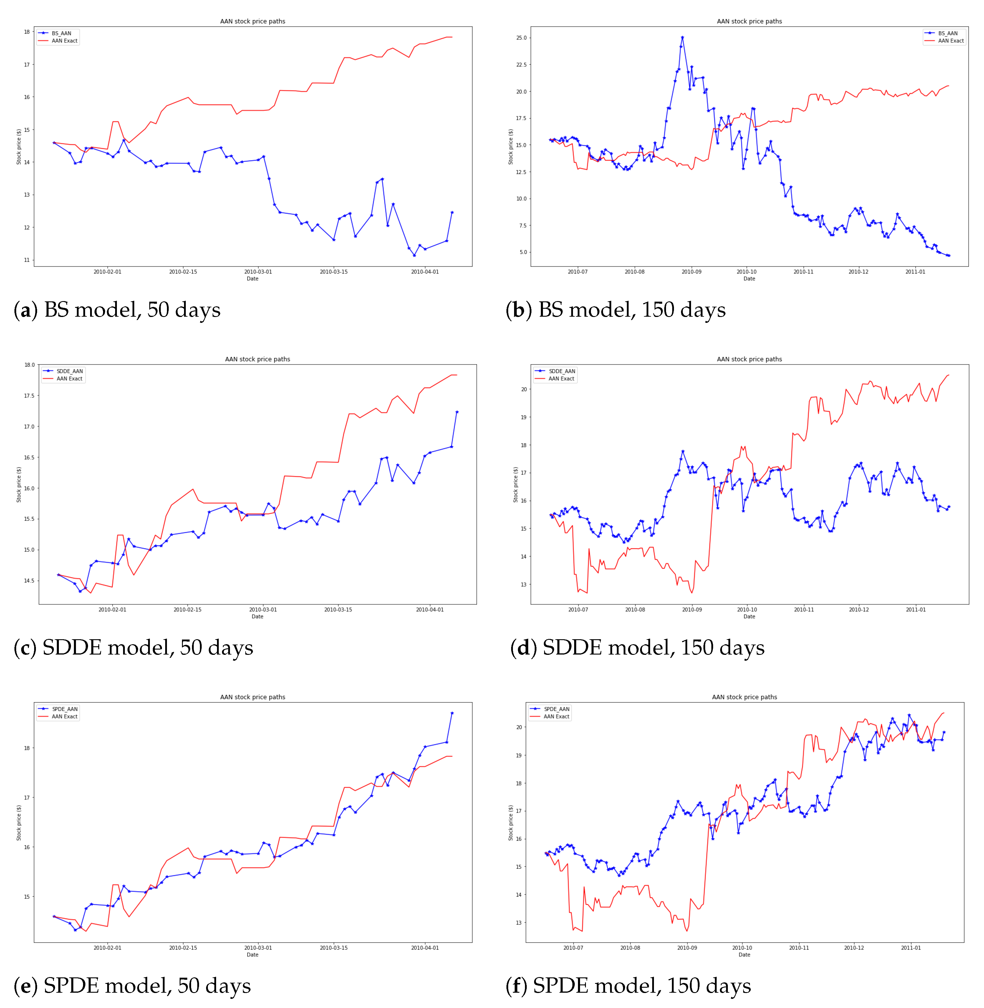
A total of 400 samples are plotted from the numerical solution for the models along with their means (blue-star curves). The curves of the stock price as a function of time are shown as (red-solid curves). The means of the numerical samples are intended (blue curves) to fit the stock price well S (thick red curves) with moderate standard derivations (small spread of the numerical samples compared to its mean); this will be the aim of the comparisons.

Fifty days from 22 January 2010 to 6 April 2010 and 150 days from 16 June 2010 to 19 January 2011 observed for the Aaron’s, Inc. (AAN Co., Atlanta, CA, USA) company were considered as the real data of the stock price. It is compared with the predicted stock price of BS, SDDE and the proposed SP-SPDE models in Figure 4. Note that the memory data of SDDE is considered as 50 and 150 days just before the observed interval. The risk-free interest rate and the time-step size are set as 0.008 and 0.03, respectively. The relating parameters in SDDE $\tau =50,150$ and SP-SPDE are $q=0.5,\sigma =1.6,\alpha =0.8$.

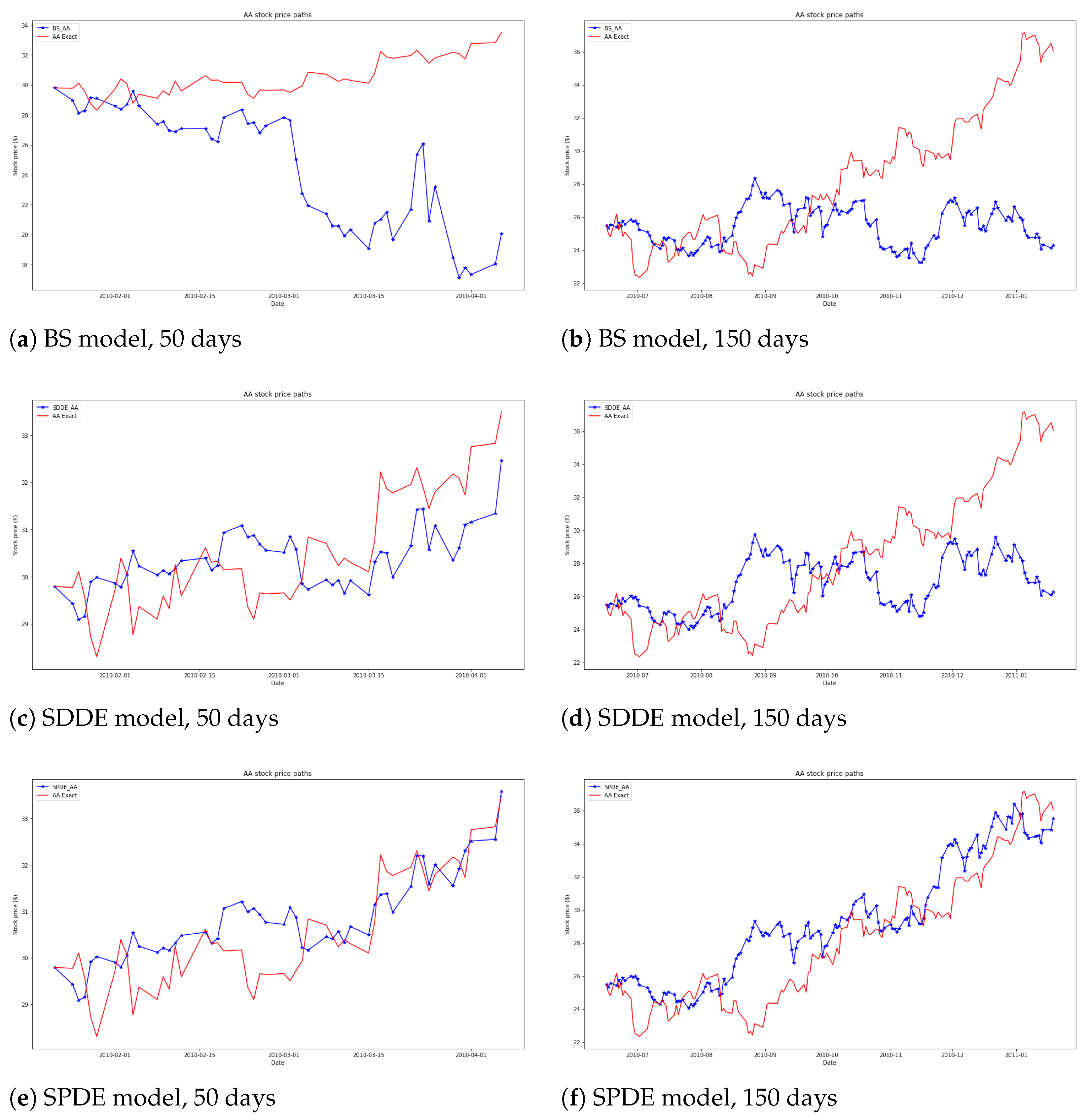
In Figure 5, 50 days from 22 January 2010 to 6 April 2010 and 150 days from 16 June 2010 to 19 January 2011 are considered as the real data observed for the Alcoa Corporation (AA Co., Pittsburgh, PA, USA) company. It is compared with the predicted stock price of the BS, SDDE and proposed SP-SPDE models. Note that the memory data of SDDE is considered as 50 and 150 days just before the observed interval. The risk-free interest rate and the time-step size are set as 0.008 and 0.03, respectively. The relating parameters in SDDE $\tau =50,150$ and SP-SPDE are $q=0.5,\sigma =2,\alpha =0.8$.

Fifty days from 1 December 2016 to 14 February 2017 and 150 days from 1 December 2016 to 9 July 2017 observed for the Tesco PLC (TSCO. L, Welwyn Garden City, UK) company were considered as the real data of the stock price. It is compared with the predicted stock price from the BS, SDDE and proposed SP-SPDE models in Figure 6. Note that the memory data of SDDE is considered as 50 and 150 days just before the observed interval. The risk-free interest rate and the time-step size are set as 0.0002 and 0.03, respectively. The relating parameters of SDDE $\tau =50,150$ and SP-SPDE simulation are set as $q=0.3,\sigma =2.3,\alpha =0.8$. Note that TSCO.L’s share price has been multiplied by $0.1$ to maintain the accuracy of the chart.

In Figure 7, the 50 days from 1 December 2016 to 14 February 2017 and 150 days from 1 December 2016 to 9 July 2017 are used as the real data observed for the Barclays PLC (BCS, London, UK) company, and it is compared with the predicted stock price of the BS, SDDE and proposed SP-SPDE models. Note that the memory data of SDDE is considered as 50 and 150 days just before the observed interval. The risk-free interest rate and the time-step size are set as 0.0002 and 0.03, respectively. The relating parameters of SDDE $\tau =50,150$ and SP-SPDE simulation are set as $q=0.3,\sigma =1.5,\alpha =0.8$.

7. Discussion

The daily stock data from Yahoo finance are used. Figure 8a shows the stock sample paths of Aaron’s. Inc. (AAN.N) and Alcoa Corporation (AA.N) from 9 November 2009 to 8 November 2019 and our prediction results are shown in Figure 4 and Figure 5. Over the considered period, the price of the two companies tends to rise. It can be seen that the prediction accuracy of the proposed model SP-SPDE with a variable delay is better than that of the SDDE model with a constant delay and the BS model with constant volatility. In Figure 8b, the data for Tesco PLC (TSCO.L) and Barclays PLC (BCS) are covered from 3 May 2016 to 1 November 2019. Over this period, the price of the two companies tends to go down, and they are considered for testing the prediction accuracy of the SP-SPDE model (see Figure 6 and Figure 7). The simulation of the stock paths shows that the proposed method is better than the others. The real data with the rise and fall of the stock price are used in order to show that the proposed SP-SPDE model is efficient for predicting 50 and 150 days of stock prices.

This is attributed to the improvement in prediction accuracy for using the past dependence volatility function based on a pantograph delay $qt$ (variable delay) in SP-SPDE (3), which, in turn, depends on the value of the stock in the recent past. For $C_1$ and $C_2$, $q=0.5$, which means that the prediction of the current stock price depends on the past stock price in the middle of the period between the current event and the starting event at all mesh prediction points in [0,T]. While for $C_3$ and $C_4$, $q=0.3$ has been used, which means that the prediction of the current stock price depends on the past stock price for a third of the period between the current event and the starting event at all mesh prediction points in [0,T]. This case is compared by using the volatility function based on a constant delay $t-\tau$ in the SDDE model (2), which means that in the case of $\tau =150$ the prediction of the current stock price depends on the past stock price at the event from 150 days ago at all mesh prediction points in [0,T].

It can be seen that the accuracy of the proposed method of the periods of stock paths with jumps can be said to be acceptable, but it is not very good compared to other periods of paths without jumps. Figure 9 shows that the stock path of AAN co. has two jumps on 29 June 2010 and 13 September 2010. It can be seen that the predicted path does not have a high accuracy close to these points compared to the other periods of the path without jumps. Therefore, in future work, the SP-SPDE model with jumps will be considered in order to discuss this point.

8. Conclusions

The SP-SPDE model was derived based on an SPDE and examined in this paper as an alternative approach to modeling stock prices. The motivation for introducing a new class of a non-constant volatility SPDE model is the estimation of the volatility function based on the variable past dependence (variable delay) in order to overcome the weaknesses of the SDDE model with a constant delay and increase the prediction accuracy. The feasibility of the proposed SP-SPDE model for simulating the stock price that will take into account the sensitivity of the model for time lag $qt$ is considered. Furthermore, it is proven that there is a numerical method that can share the non-negativity feature of the proposed models’ solution. Finally, the model is tested using real data, and the results are compared with that of the SDDE model with a constant delay and a classic BS model in order to show that the proposed model could improve the prediction accuracy.

In future work, we will extend the SPDE to modeling the corporate claim value. Furthermore, the robust numerical method based on the balanced technique will be discussed to meet the non-negativity solution. Using the real financial corporate data, we will compare the accuracy of the numerical solution based on the balanced technique with that of the stochastic theta method.

References

- Black, F.; Scholes, M.S. The Pricing of Options and Corporate Liabilities. J. Pol. Econ. 1973, 81, 637–654. [Google Scholar] [CrossRef] [Green Version]
- Scott, L.O. Option pricing when the variance changes randomly: Theory, estimation, and an application. J. Financ. Quant. Anal. 1987, 22, 419–438. [Google Scholar] [CrossRef]
- Hobson, D.G.; Rogers, L.C. Complete models with stochastic volatility. Math. Financ. 1998, 8, 27–48. [Google Scholar] [CrossRef]
- Arriojas, M.; Hu, Y.; Mohammed, S.A.; Pap, G. A delayed Black and Scholes formula. Stoch. Anal. Appl. 2007, 25, 471–492. [Google Scholar] [CrossRef] [Green Version]
- Mao, X.; Sabanis, S. Delay geometric Brownian motion in financial option valuation. Stoch. Int. J. Prob. Stoch. Process. 2013, 85, 295–320. [Google Scholar] [CrossRef] [Green Version]
- Lin, L.; Li, Y.; Wu, J. The pricing of European options on two underlying assets with delays. Phys. A-Stat. Mech. Its Appl. 2018, 495, 143–151. [Google Scholar] [CrossRef]
- Liu, C. Basic theory of a class of linear functional differential equations with multiplication delay. arXiv 2016, arXiv:1605.06734. [Google Scholar]
- Eissa, M.A.; Tian, B. A stochastic corporate claim value model with variable delay. J. Phys. Conf. Ser. 2018, 1053, 12–18. [Google Scholar] [CrossRef]
- Wang, X. Some theoretical results on the stability of uncertain pantograph differential equations. J. Intell. Fuzzy Syst. 2020, 38, 4431–4439. [Google Scholar] [CrossRef]
- Xiao, Y.; Eissa, M.A.; Tian, B. SConvergence and stability of split-step theta methods with variable step-size for stochastic pantograph differential equations. Int. J. Comput. Math. 2018, 95, 939–960. [Google Scholar] [CrossRef]
- Kahl, C. Positive Numerical Integration of Stochastic Differential Equations. Diploma Thesis, University of Wuppertal, Wuppertal, Germany, 2004; pp. 46–57. [Google Scholar]
- Tambue, A.; Brown, E.K.; Mohammed, S. A stochastic delay model for pricing debt and equity: Numerical techniques and applications. Commun. Nonlinear Sci. Num. Simul. 2015, 20, 281–297. [Google Scholar] [CrossRef] [Green Version]
- Eissa, M.A.; Tian, B. Lobatto-milstein numerical method in application of uncertainty investment of solar power projects. Energies 2017, 10, 43. [Google Scholar] [CrossRef] [Green Version]
- Eissa, M.A.; Zhang, H.; Xiao, Y. Mean-square stability of split-step theta milstein methods for stochastic differential equations. Math. Probl. Eng. 2018, 2018, 1682513. [Google Scholar] [CrossRef]
- Eissa, M.A. Mean-square stability of two classes of theta milstein methods for nonlinear stochastic differential equations. Proc. Jangjeon Math. Soc. 2019, 22, 119–128. [Google Scholar]
- Eissa, M.A.; Ye, Q. Convergence, non-negativity and stability of a new Lobatto IIIC-Milstein method for a pricing option approach based on stochastic volatility model. Jpn. J. Ind. Appl. Math. 2021, 38, 391–424. [Google Scholar] [CrossRef]
- Higham, D.J.; Mao, X.; Szpruch, L. Convergence, Non-negativity and Stability of a New Milstein Scheme with Applications to Finance. Discret. Contin. Dyn. Syst.-Ser. B 2013, 18, 2083–2100. [Google Scholar] [CrossRef]
- Kahl, C.; Schurz, H. Balanced Milstein Methods for Ordinary SDEs. Monte Carlo Methods Appl. 2006, 12, 143–170. [Google Scholar] [CrossRef]
- Tian, B.; Eissa, M.A.; Zhang, S. Two families of theta milstein methods in a real options framework. In Proceedings of the 5th Annual International Conference on Computational Mathematics, Computational Geometry and Statistics (CMCGS 2016), Singapore, 18–19 January 2016; pp. 18–19. [Google Scholar]
- Aghda, A.F.; Hosseini, S.M.; Tahmasebi, M. Analysis of non-negativity and convergence of solution of the balanced implicit method for the delay Cox-Ingersoll-Ross model. Appl. Num. Math. 2017, 118, 249–265. [Google Scholar] [CrossRef]
- Dangerfield, C.E.; Kay, D.; Macnamara, S.; Burrage, K. A boundary preserving numerical algorithm for the Wright-Fisher model with mutation. BIT Num. Math. 2012, 52, 283–304. [Google Scholar] [CrossRef] [Green Version]
- Moro, E.; Schurz, H. Boundary preserving semianalytic numerical algorithms for stochastic differential equations. SIAM J. Sci. Comput. 2007, 29, 1525–1549. [Google Scholar] [CrossRef] [Green Version]
- Xiao, F.; Qin, T.; Zhang, C. Mean-square stability of Milstein methods for stochastic pantograph equations. Math. Probl. Eng. 2013, 2013, 724241. [Google Scholar] [CrossRef] [Green Version]
- Kemajou, E.; Mohammed, S.A.; Tambue, A. A Stochastic Delay Model for Pricing Debt and Loan Guarantees: Theoretical results. arXiv 2012, arXiv:1210.0570. [Google Scholar]
- Mao, X. Stochastic Differential Equations and Applications; Woodhead Publishing: Sawston, UK, 2011. [Google Scholar]
- Fan, Z.; Liu, M.; Cao, W. Existence and uniqueness of the solutions and convergence of semi-implicit Euler methods for stochastic pantograph equations. J. Math. Anal. Appl. 2007, 325, 1142–1159. [Google Scholar] [CrossRef] [Green Version]
- Rouz, O.F.; Ahmadian, D.; Milev, M. Exponential mean-square stability of two classes of theta Milstein methods for stochastic delay differential equations. AIP Conf. Proc. 2017, 1910, 060015. [Google Scholar]
Figure 1.
Description of the concept of constant delay .
Figure 2.
Description of the concept of variable delay .
Figure 3.
Stock sample paths using SDDE with memory interval time.
Figure 4.
The graphs for corporation AAN co. 50 and 150 days are shown on the left and right, respectively. The top (a,b) corresponds to the BS model, while the middle (c,d) corresponds to the SDDE model with a constant delay , and the graphs at the bottom (e,f) correspond to the SP-SPDE model with a variable delay .
Figure 5.
The graphs for corporation AA co. 50 and 150 days are shown on the left and right, respectively. The top (a,b) corresponds to the BS model, while the middle (c,d) corresponds to the SDDE model with a constant delay , and the graphs at the bottom (e,f) correspond to the SP-SPDE model with a variable delay .
Figure 6.
The graphs for corporation Tesco PLC 50 and 150 days are shown on the left and right, respectively. The top (a,b) corresponds to the BS model, while the middle (c,d) corresponds to the SDDE model with a constant delay , and the graphs at the bottom (e,f) correspond to the SP-SPDE model with a variable delay .
Figure 7.
The graphs for corporations and at the top (a,b) correspond to the BS model, while the graphs in the middle (c,d) correspond to the SDDE model with a constant delay with memory data , and the graphs at the bottom (e,f) correspond to the SP-SPDE model with a variable delay .
Figure 8.
Stock sample paths.
Figure 9.
Stock sample paths of AAN co. with jumps.
Publisher’s Note: MDPI stays neutral with regard to jurisdictional claims in published maps and institutional affiliations. |
© 2022 by the authors. Licensee MDPI, Basel, Switzerland. This article is an open access article distributed under the terms and conditions of the Creative Commons Attribution (CC BY) license (https://creativecommons.org/licenses/by/4.0/).
Share and Cite
MDPI and ACS Style
Eissa, M.A.; Elsayed, M. Improve Stock Price Model-Based Stochastic Pantograph Differential Equation. Symmetry 2022, 14, 1358. https://0-doi-org.brum.beds.ac.uk/10.3390/sym14071358
AMA Style
Eissa MA, Elsayed M. Improve Stock Price Model-Based Stochastic Pantograph Differential Equation. Symmetry. 2022; 14(7):1358. https://0-doi-org.brum.beds.ac.uk/10.3390/sym14071358
Chicago/Turabian StyleEissa, Mahmoud A., and M. Elsayed. 2022. "Improve Stock Price Model-Based Stochastic Pantograph Differential Equation" Symmetry 14, no. 7: 1358. https://0-doi-org.brum.beds.ac.uk/10.3390/sym14071358
Note that from the first issue of 2016, this journal uses article numbers instead of page numbers. See further details here.