
A Novel Inverse Credibility Distribution Approach for the Membership Functions of LR Fuzzy Intervals: A Case Study on a Completion Time Analysis

The Research Center of Energy Economy, School of Business Administration, Henan Polytechnic University, Jiaozuo 454150, China
Symmetry 2022, 14(8), 1554; https://0-doi-org.brum.beds.ac.uk/10.3390/sym14081554
Submission received: 28 June 2022
/
Revised: 17 July 2022
/
Accepted: 26 July 2022
/
Published: 28 July 2022
(This article belongs to the Special Issue Fuzzy Set Theory and Uncertainty Theory)
Abstract
:Fuzzy arithmetic is of great significance in dealing with vague information, especially the basic arithmetic operations (i.e., ⊕, ⊖, ⊗, ⊙). However, the classical and widely accepted accurate and approximate approaches, the interval arithmetic approach and standard approximation method, cannot output accurate or well-approximated expressions of the membership function, which may prevent decision makers from making the right decisions in real applications. To tackle this problem, this paper first discusses the relationships among the membership function, the credibility distribution, and the inverse credibility distribution and summarizes the relationships as several theorems. Then, by means of the theorems and the newly proposed operational law, this paper proposes an inverse credibility distribution approach that can output the accurate expression of the membership function for continuous and strictly monotone functions of regular fuzzy intervals. To better demonstrate the effectiveness of the raised approach, the commonly-used fuzzy interval, the symmetric trapezoidal fuzzy number, is employed, and several comparisons with the other two methods are made. The results show that the proposed approach can output an exact or well-approximated expression of the membership function, which the others cannot. In addition, some comparisons of the proposed approach with other methods are also made on a completion time analysis of a construction project to show the effectiveness of the proposed approach in real applications.
1. Introduction
Since Zadeh’s previous work on fuzzy set theory [1], fuzzy sets have become a strong tool in the description of incomplete and uncertain situations. By now, various fuzzy sets have been proposed, such as linear Diophantine fuzzy sets [2] and spherical linear Diophantine fuzzy sets [3], and have already assisted people in solving various important practical problems, among which the fuzzy interval [4], one of of the famous fuzzy sets and with decreasing shape functions L and R, has attracted research attention. In real applications, the arithmetic operations (i.e., ⊕, ⊖, ⊗, ⊙) of the fuzzy intervals are of great significance, since the accuracy of the obtained results can influence the choice of decision schemes and improper ones may result in huge loss. However, Zadeh’s extension principle, the fundamental arithmetic for the above arithmetic operations, contains the operations and , which means the arithmetic operations can be non-linear, tedious calculation, and difficult to be applied. In view of this, from the perspective of simplifying the computational process, the approximate and exact methods of fuzzy arithmetic operations emerge.
The initial approximate method for fuzzy intervals was proposed by Dubois and Prade [5] by the use of a fuzzification principle, and its practical use reduces computational complexity and is shown to be easily followed. However, too frequent use of the multiplication of the method may lead to extensive damage due to an inaccurate membership function. To tackle this problem, subsequent scholars have carried out a great deal of work to reduce the error generated from the approximate method. By the utilization of the values of triangular and trapezoidal fuzzy numbers (two kinds of fuzzy numbers), Giachetti and Young [6] developed a new approximation method, and the error generated from the approximate method in [5] was reduced by a large margin. Guerra and Stefanini [7] developed a novel procedure to reduce the computational error produced among the arithmetic operations between fuzzy intervals by using the piecewise monotonic interpolations. Ban et al. [8] integrated the weighted average Euclidean distance into the approximation of the arithmetic operation of fuzzy numbers, and the examples demonstrate that the developed method can output more accurate results. With the help of the approximate methods, some practical problems were well solved, such as multi-criteria decision-making [9], risk analysis [10], and so on.
Although the simple and easy-followed characters make the approximate method famous, the error between the obtained results and the exact ones always exist and sometimes may lead to the production of an extremely large erroneous result. In view of this, the accurate fuzzy arithmetic operations have come into being. As regards the triangular and trapezoidal fuzzy number, Kaufmann and Gupta [11] studied the relationship between the -cuts points and the arithmetic operations and then proposed the widely accepted interval arithmetic approach [12,13]. However, this method may lead to higher powers of as the number of the multiplied fuzzy terms increases and cannot acquire the expression of the corresponding membership functions. By means of the credibility measure [14] and the newly-proposed operational law [15], Xie et al. [16] proposed an inverse distribution approach for the arithmetic of triangular fuzzy numbers, and the results show that the approach can output not only the membership functions as [11] but also the corresponding exact expressions. As clearly can be seen from the accurate methods, studies on accurate fuzzy arithmetic operations are rare, and the scope of their application is only restricted to some special fuzzy numbers (i.e., triangular or trapezoidal fuzzy numbers).
Considering that a fuzzy arithmetic operation method that has a wide application scope and can output exact expression of the membership function may make a big difference in real applications, such as decision making, fuzzy optimization, and so on, this paper chooses the frequently-encountered regular fuzzy intervals as the main object and then exploits an operational law of the regular fuzzy intervals [17] based approach for the membership functions of functions of fuzzy intervals (i.e., the inverse credibility distribution approach), in which the inverse credibility distributions of functions of fuzzy intervals are first managed by the operational law [17]; then, by studying the relationship between the membership function and the two distributions (the credibility and inverse credibility distribution), the expressions of the membership functions of functions of fuzzy intervals are finally exported. The contributions of this paper are mainly in the following three aspects: (1) some theorems concerning the membership function, the credibility distribution, and the inverse credibility distribution of regular fuzzy intervals are developed; (2) we develop an inverse credibility distribution approach for the exact expressions of the membership functions of functions of fuzzy intervals, which can applied to any regular fuzzy intervals with continuous and strictly monotone functions; (3) in order to reflect the effectiveness of the proposed method, some numerical examples, together with a completion time analysis incorporating the commonly-used fuzzy interval (trapezoidal fuzzy number), are conducted, in which the classic standard approximate method [5], interval arithmetic approach [11], and fuzzy simulation approach [18] are chosen to make a comparison.
The rest of the paper is organized as follows. Section 2 introduces the basic concepts of the regular fuzzy interval, involving the credibility measure, credibility and inverse credibility distribution, and the operational law. By discussing the relationships among the membership function and the two distributions, the inverse credibility distribution approach is presented in Section 3. Some examples concerning the symmetric trapezoidal fuzzy numbers are listed in Section 4 to demonstrate the effectiveness of the approach in this paper. The proposed approach is further applied to a completion time analysis of a construction project in Section 5.
2. Preliminaries
In this section, some related knowledge concerning the membership function, credibility distribution, inverse credibility distribution, and the operational law of regular fuzzy intervals is recalled.
2.1. Regular Fuzzy Interval
Dubois and Prade [4] initialized the fuzzy interval, which has four parameters: , , and the membership function,
where L and R are the shape functions for left and right (see for [4,17,19] for more details), respectively. Among the fuzzy intervals, a special type, continuous and strictly monotone in regard to and , has attracted researchers’ attention, as applied in [20,21,22] with well-appreciated results. Liu et al. [23] named this kind of fuzzy interval the regular fuzzy interval.
Definition 1
(Liu et al. [23]). Provided that the shape functions L and R are continuous and strictly decrease with regard to t where and , then the fuzzy interval is regular.
Example 1.
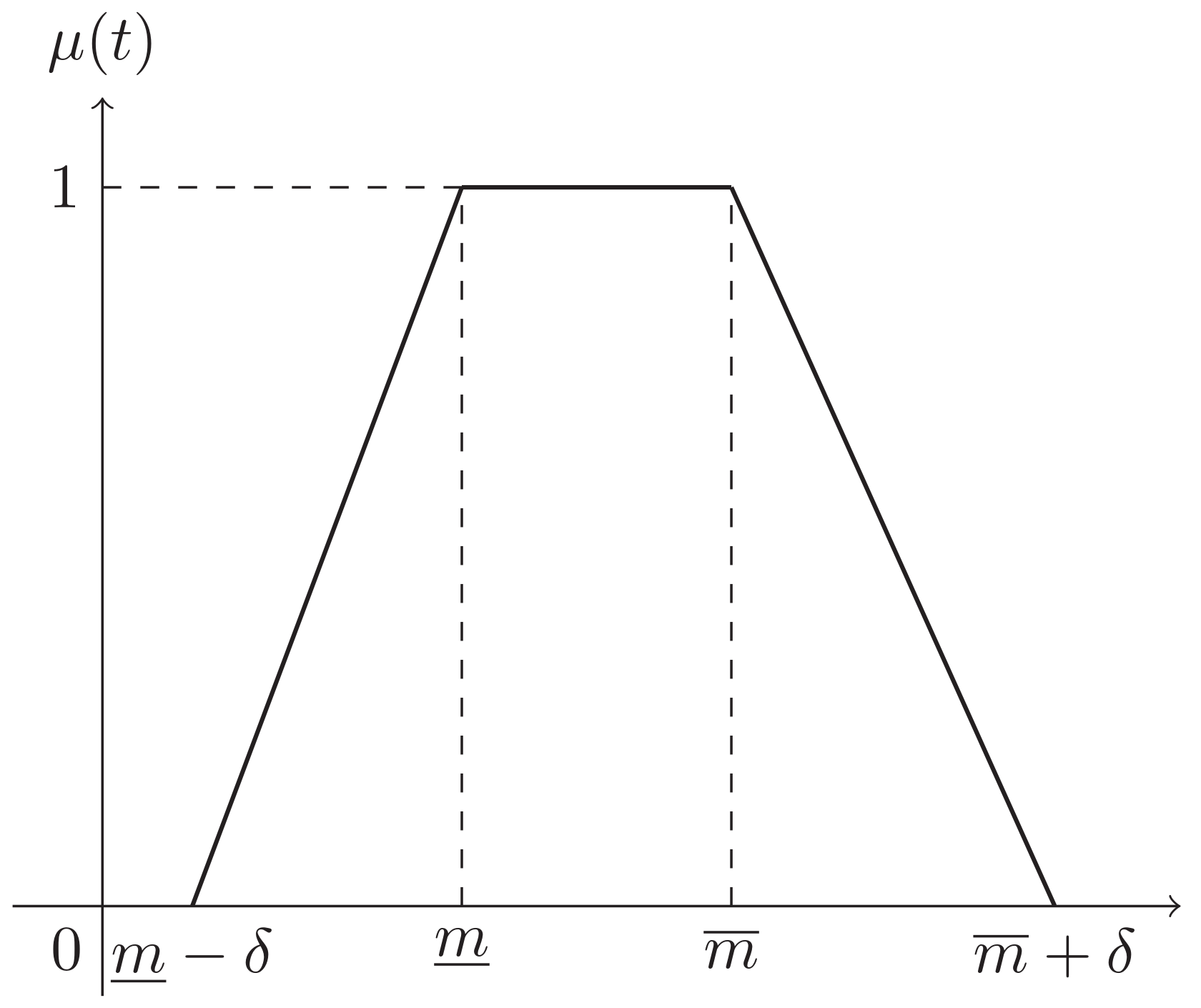
If a fuzzy interval ξ has shape functions and the membership function
where l and k are the boundaries of the interval that the possibility value of ξ is 1, then ξ is a trapezoidal fuzzy number (TFN). Note that the TFN ξ is said to be symmetric if . Denote that , and a symmetric TFN ξ is symbolized by which is depicted in Figure 1.
2.2. Credibility and Inverse Credibility Distribution
Considering the lack of self-duality in the possibility measure (Pos) [24] and necessity measure (Nec) [25], Liu and Liu [14] raised the credibility measure (Cr), which is the average of the above two measures, i.e., . For any fuzzy number , the credibility of the fuzzy events is
where r is a real number, , and . With the help of the credibility measure, Liu [26] proposed the credibility distribution , which is,
By means of Equations (1)–(3), we can obtain the credibility distribution of a fuzzy interval ; that is,
Example 2.
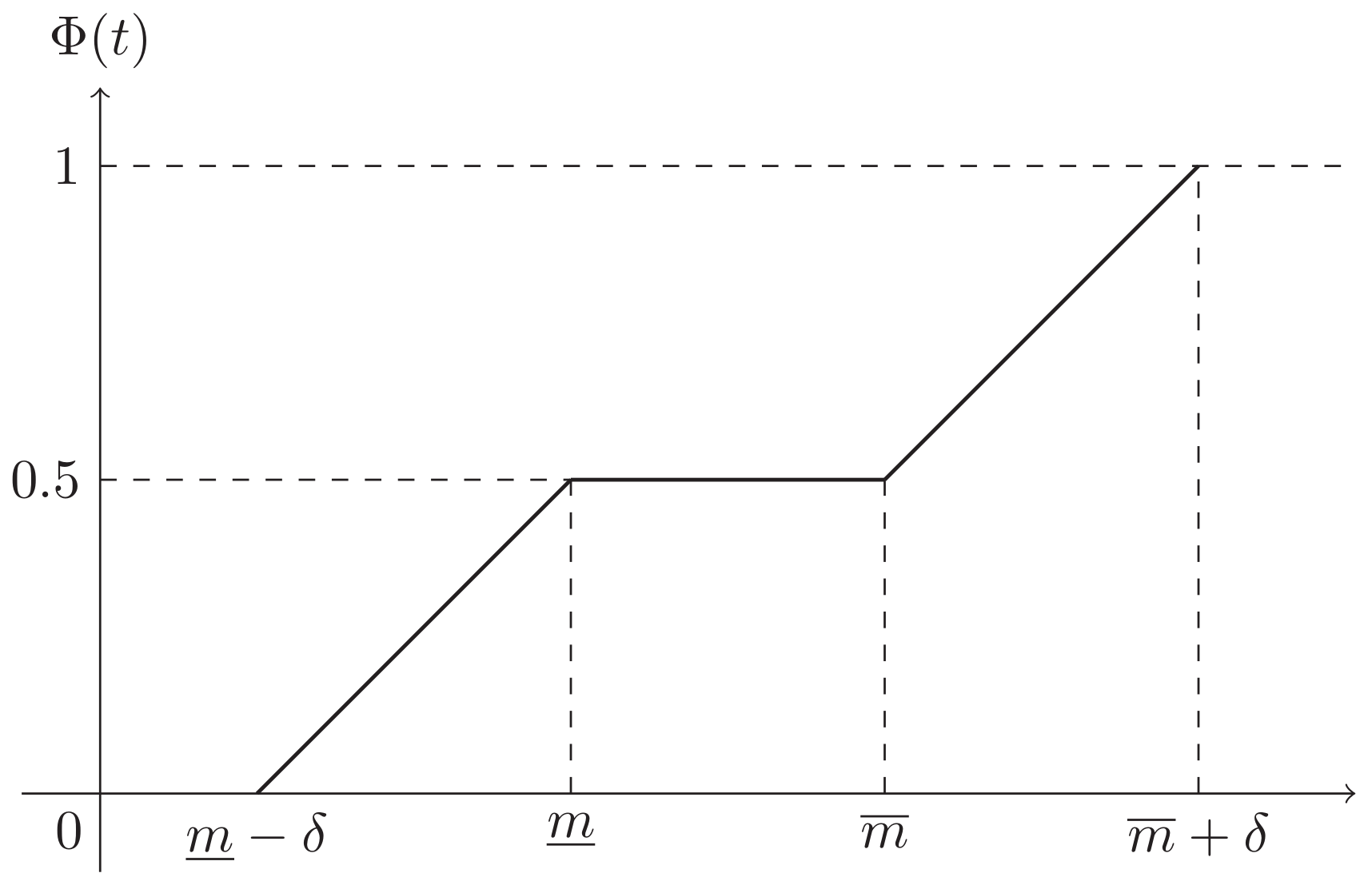
The credibility distribution of the symmetric trapezoidal fuzzy number is,
the representation of which can be seen in Figure 2.
From Figure 2, the shape of the credibility distribution is continuous and strictly increasing with respect to and . By virtue of such superior properties, Zhao et al. [17] proposed the concept of the inverse credibility distribution.
Theorem 1
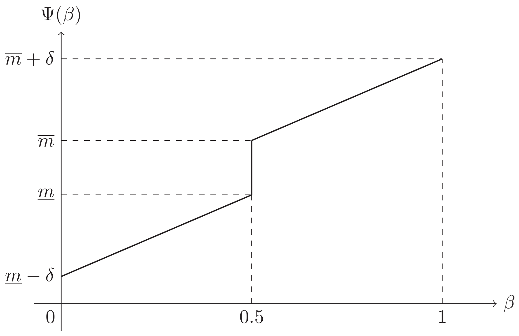
(Zhao et al. [17]). Provided that a regular fuzzy interval ξ has four parameters , , ν, and η, the inverse credibility distribution is
Example 3.
2.3. The Operational Law of Regular Fuzzy Intervals
As can be seen from Section 2.2, the membership function, credibility distribution, and the inverse credibility distribution of regular fuzzy intervals have praiseworthy properties, i.e., they are continuous and strictly monotone with respect to and or and . In view of this, Zhao et al. [17] further explored them and then proposed the operational law for the inverse credibility distribution of functions of regular fuzzy intervals, which is as follows.
Theorem 2
(Zhao et al. [17]). Let be regular fuzzy intervals, with inverse credibility distributions . If the continuous function is strictly increasing with regard to and strictly decreasing with regard to , , then is a regular fuzzy interval and has an inverse credibility distribution:
Example 4.
Denote , , and . Then, compute the inverse credibility distribution of .
From Equation (4), we can obtain that is
Since the function f is continuous and strictly increasing with respect to and decreasing with respect to , we can obtain the inverse credibility distribution of ξ from Theorem 2; that is,
3. The Novel Inverse Credibility Distribution Approach
In this section, the relationship of the membership function , the credibility distribution , and inverse credibility distributions of a regular fuzzy interval is first discussed. Then, with the assistance of the operational law in [17], the inverse credibility distribution approach for the membership function of the regular fuzzy interval, , is conducted, where the function is continuous and strictly monotone with respect to .
3.1. The Relationship of , , and of a Regular Fuzzy Interval
Theorem 3.
Denote that ξ is a regular fuzzy interval, which has membership function μ and credibility distribution Φ; then, we have
where and are the lower and upper modal values.
Proof.
To prove Theorem 3, three cases should be discussed, which are as follows.
Case 1: . It follows from the definition of the credibility distribution and credibility measure that we have
By virtue of Zadeh’s extension principle, we then have
Because the sharp function is continuous and strictly increasing with regard to , we can obtain
Finally, we have .
Case 2: . It is obvious that .
Case 3: . The procedure for the proof is the same as Case 1. □
It can be clearly observed from Theorem 3 that the membership function and the credibility distribution can be transferred mutually; that is, once the expression of or is obtained, the other can be deduced immediately.
Theorem 4.
Denote that ξ is a regular fuzzy interval, which has credibility distribution Φ and inverse credibility distribution Ψ; then, we have
where is the inverse function of the inverse credibility distribution Ψ.
Proof.
From [17], for a regular fuzzy interval, its inverse credibility distribution is continuous and strictly increasing with regard to or . It follows from the continuity and monotonicity that .
Based on Definition 1, we have as . For all of these, Theorem 4 holds. □
From Theorem 4, the functions of the two distributions also have a one-to-one relationship in and , owing to the continuity and strict monotonicity of the credibility distribution and inverse credibility distribution in this domain. Therefore, we can deduce the expression of one of the two distributions and if the other one is known. Considering Theorems 3 and 4 comprehensively, if the inverse credibility distribution is found, by using the relationship among the two distributions ( and ) and the membership function (), we can acquire the expression of with little hindrance. Inspired by this, supposing that f is continuous and strictly monotone in regard to , resorting to the relationship among , and , we can output the expression of the membership function of by virtue of the inverse credibility distribution obtained by Theorem 2. However, there exists a gap regarding whether the inverse credibility and the credibility distribution of are in a one-to-one relationship or not, which is discussed in the following.
Theorem 5.
Let be independent regular fuzzy intervals with credibility distributions . If the continuous function is strictly increasing with regard to and strictly decreasing with regard to , , then the inverse credibility distribution Ψ of exists and is continuous and strictly increasing in or .
Proof.
Without loss of generality, denote that , where f is continuous and strictly increasing with respect to and decreasing to . From Theorem 2, we have
From Definition 1, we can deduce that is strictly increasing and is decreasing with respect to in or . For any two points and with , we have
and
Since the function f is continuous and strictly increasing with respect to and decreasing with respect to , we have
That is, .
Since f and are both continuous in or , the inverse credibility distribution is obviously continuous. □
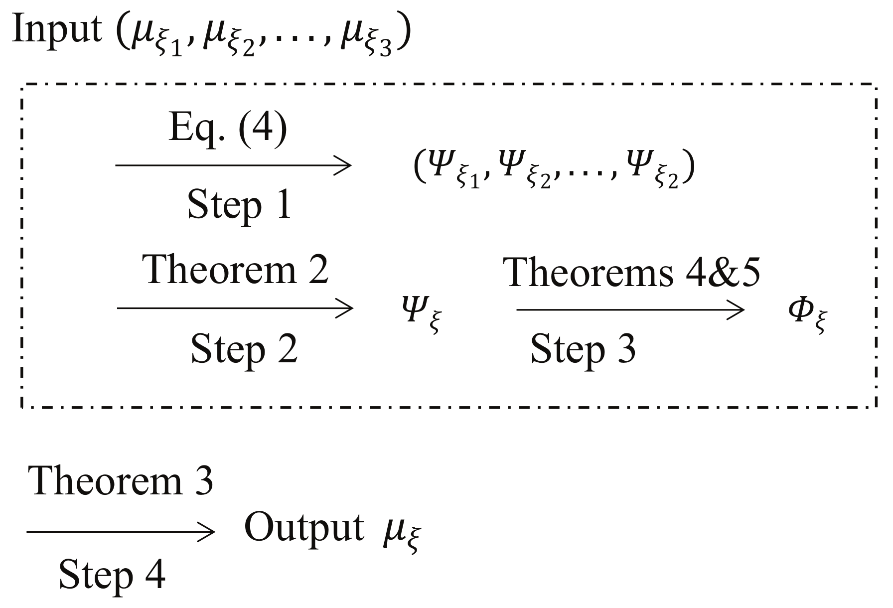
Clearly, from Theorem 5, the two distributions (credibility and inverse credibility distribution) of functions of are in a one-to-one relationship. Theorems 3–5 provide an idea for the acquisition of the expression of the membership function of functions of regular fuzzy intervals, which is depicted in Figure 4.
Based on the idea, we proposed an inverse credibility distribution approach for the membership function of function f involving regular fuzzy intervals, where f is continuous and of strict monotonicity, and the details are presented in the following section.
3.2. The Steps of the Inverse Credibility Distribution Approach
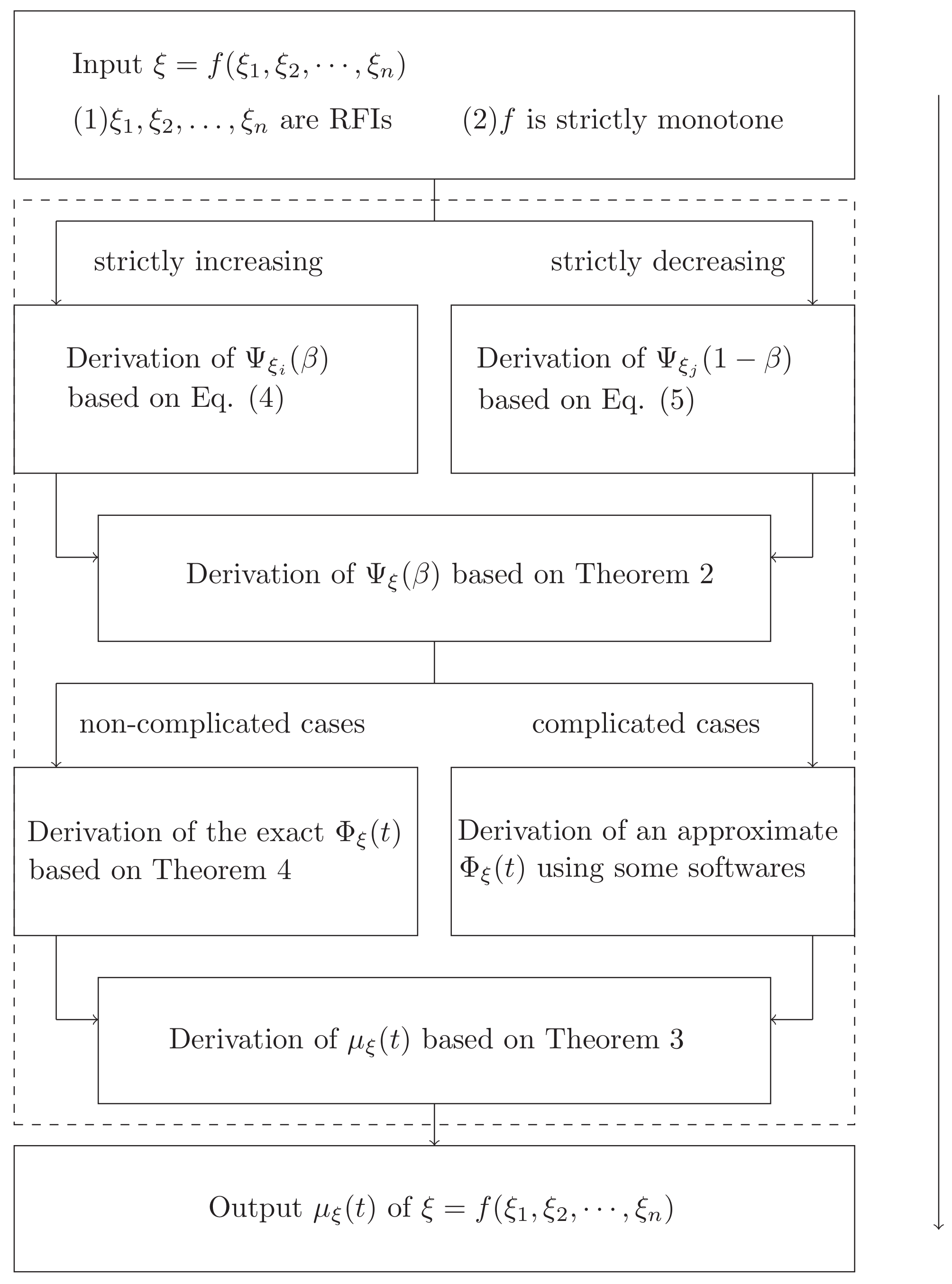
Let , be regular fuzzy intervals (RFIs), and f is continuous and of strict monotonicity. Then, the membership function of can be deduced by means of the inverse credibility distribution approach, the steps of which are presented in the following.
Step 1: Derive the inverse credibility distributions of , , when the function f is strictly increasing, and of , as f is strictly decreasing, by using Equations (4) and (5).
Step 2: Use the operational law (i.e., Theorem 2) to acquire the inverse credibility distribution of .
Step 3: Derive the credibility distribution of by by using Theorem 4. There exists an inverse procedure in the acquisition of the credibility distribution , and this procedure may not proceed when the inverse credibility distribution is complex. To handle this problem, this step is divided into two parts: use the inverse approach (i.e., Theorem 4) to obtain the credibility distribution of in the case of simple , and utilize the function `polyfit’ (input the expression of , and a well-approximated expression for would be outputted immediately) in MATLAB with the version of ”2015a” to acquire the credibility distribution fo complex .
Step 4: Output the membership function of by taking advantage of the relationships of the credibility distribution and the membership function (i.e., Theorem 3).
The steps of the inverse credibility distribution approach are summarized in a flowchart (see Figure 5). To better describe the procedures of the inverse credibility distribution approach, the next section uses the frequently-used symmetrical TFN as an example.
4. Numerical Example
In this section, to clearly demonstrate the usage of the proposed approach, five examples, similar to many other references that studied fuzzy arithmetics, for symmetric TFN are designed. The first example is used to show the effectiveness of the approach with different types of regular fuzzy intervals, and the five examples are presented to show the influence of different kinds of functions, where the last two examples are used to demonstrate the implementation of the approach by the usage of some developed software. Besides the classical and widely-used accurate and approximate approaches, the standard approximate method and interval arithmetic approach are also introduced, and their results are also displayed graphically to clarify the effectiveness and correctness of the inverse credibility distribution approach.
Example 5.
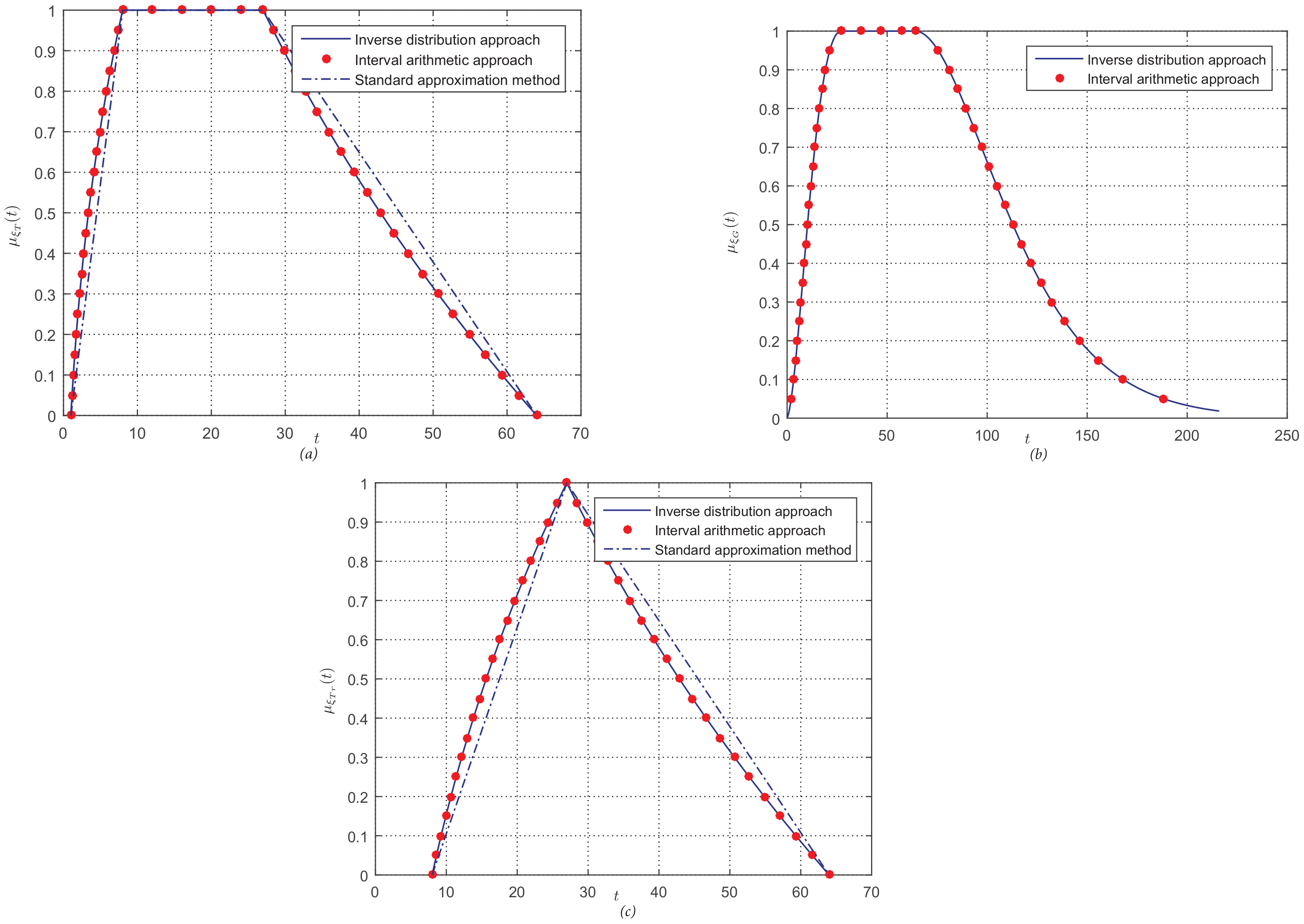
This example employs the Gaussian fuzzy interval (G), triangular fuzzy number (), and trapezoidal fuzzy number (T) to show the effectiveness of the proposed approach. Let be the three kinds of regular fuzzy intervals and be .
Let the three parameters , and δ of the symmetric trapezoidal number be 3, 2, and 1, and then compute the membership function of . Owing to the continuity and strict increase of the function f, we can gain the inverse credibility distribution by means of Equation (4), which is
According to Theorem 2, the inverse credibility distribution of ξ is
From Theorem 4, the credibility distribution is obtained by means of a inverse procedure; that is,
In view of Theorem 3, the membership function of ξ is
Let be a Gaussian fuzzy interval, where the four parameters , , ν, and η are 3, 4, 1, and 1; then, we can obtain the membership function of by using a similar procedure; that is,
Let be a triangular fuzzy number, where the left and right boundaries (a,c) and median value b are 2, 4, 3; then, we can obtain the membership function of by using a similar procedure; that is,
In this example, the results of the standard approximate method and interval arithmetic approach are also calculated and represented in Figure 6, and we can clearly see the performance of the membership function. In Figure 6, the symbols “−”, “•”, and “” represent the membership functions of the inverse credibility distribution approach, the interval arithmetic approach, and the standard approximation method, and , , and illustrate the membership functions of the trapezoidal fuzzy number, Gaussian fuzzy interval, and triangular fuzzy number, respectively. It should be noted that the cuts points are the main basis of the interval arithmetic approach; that is, a set of cuts points should be predetermined and then the arithmetic rules used to acquire the accurate points in membership function, which means that the membership function from the interval arithmetic approach is discrete and not continuous. The values of h are set to , and the corresponding membership function of the interval arithmetic approach is presented in Figure 6. Obviously, the “•” points all fall into the blue line “−” in all of the three graphs, which demonstrates the accuracy of the membership function from the inverse credibility distribution approach. The distances of the membership function from the standard approximate method to the interval arithmetic are large, especially in the right part, and the standard approximate method cannot be applied to the Gaussian fuzzy interval. For all inputs, the proposed inverse credibility distribution approach can output the accurate expression of the membership function of functions of regular fuzzy intervals, regardless of the type of fuzzy intervals. As a result, the following discusses the performance of the approach with different functions.
Example 6.
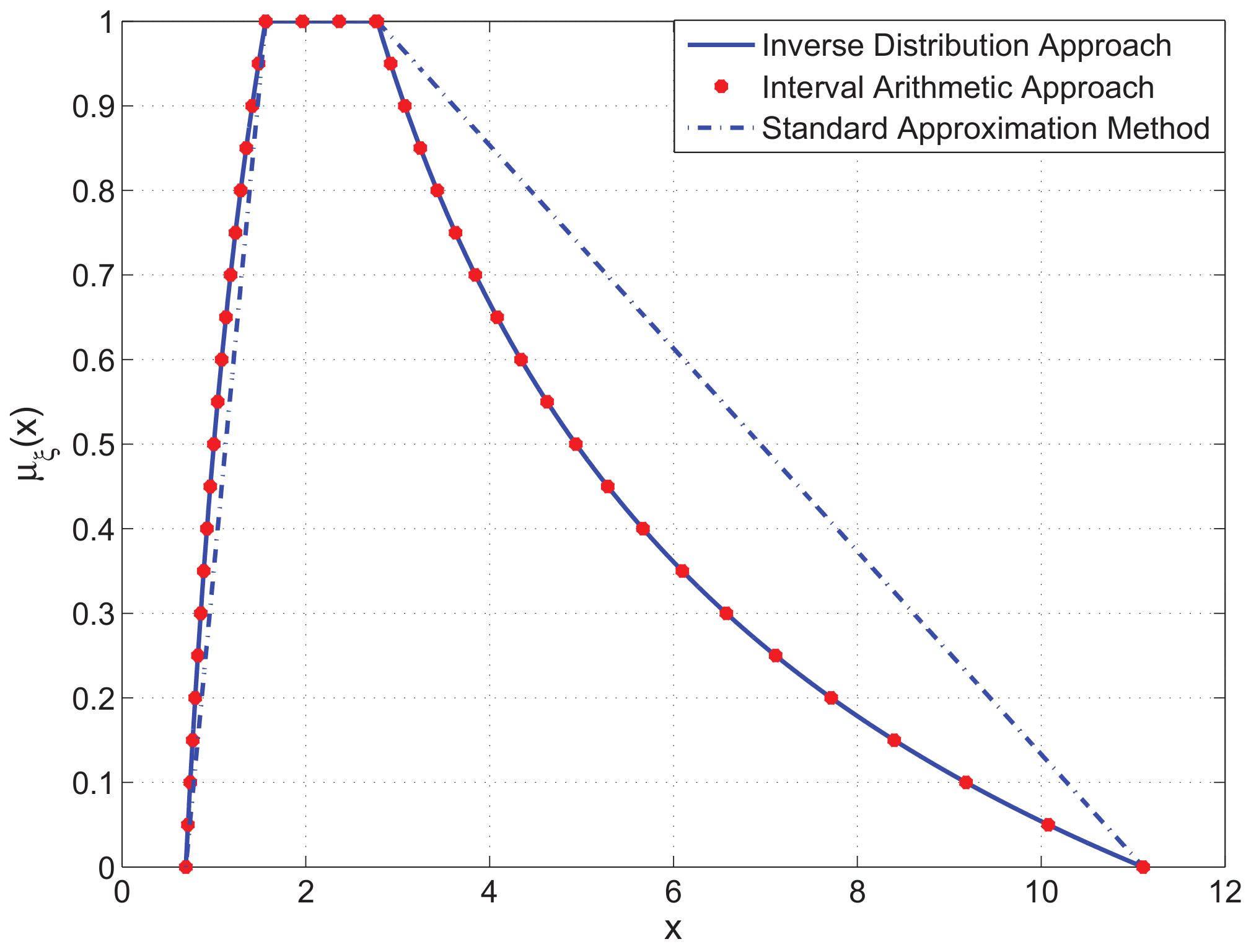
Let and is . Then, output the membership function of .
The three parameters , and δ of the symmetric trapezoidal number are 0.8, 0.6, and 0.3. Owing to the continuity and strict increase of the function f, by means of Equation (4) and Theorem 2, the inverse credibility distribution is
In view of Theorem 4, the credibility distribution of ξ is
Based on Theorem 3, we can obtain the membership function :
The membership functions of the three approaches are all summarized in Figure 7. The values of h in the interval arithmetic approach are also set to , and the obtained membership function is represented by the symbol “•”. In the same way as the former example, the membership function from the inverse credibility distribution also has praiseworthy accuracy, since the “−” symbols penetrate all of the “•” symbols. The standard approximation method has poor performance in the accuracy of the membership function due to the large distance from the “” (representing the membership function of the standard approximation method) to the “−” and “•” in .
Example 7.
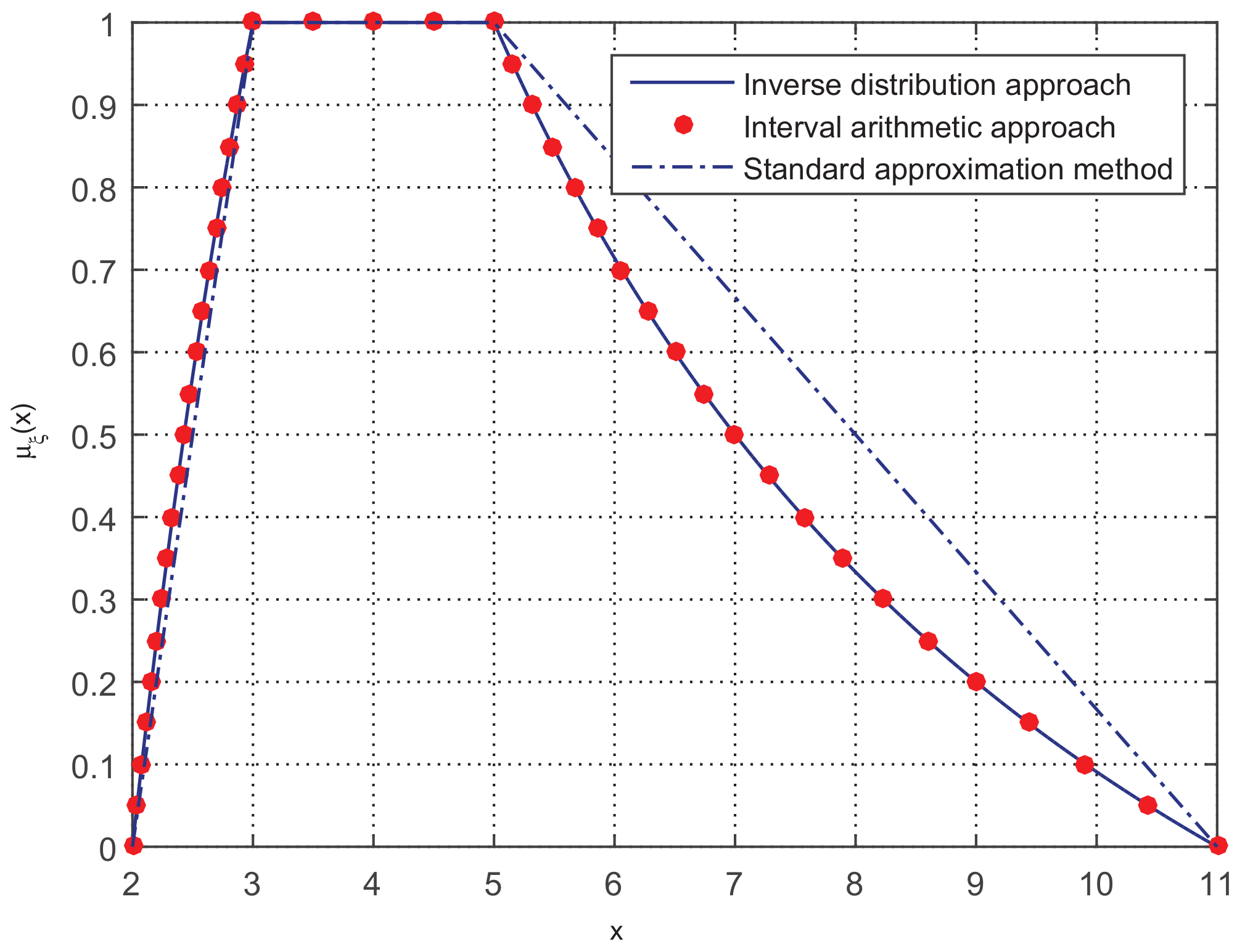
Let , and . Then, compute the membership function of .
The three parameters , , and δ of the symmetric trapezoidal numbers and are 9, 10, 1, and 2, 3, 1, respectively. Owing to the continuity and strict monotonicity of the function f, by means of Equation (4), we can output the inverse credibility distribution :
On account of Theorem 4, we can obtain the credibility distribution :
Then, from Theorem 3, the membership function is
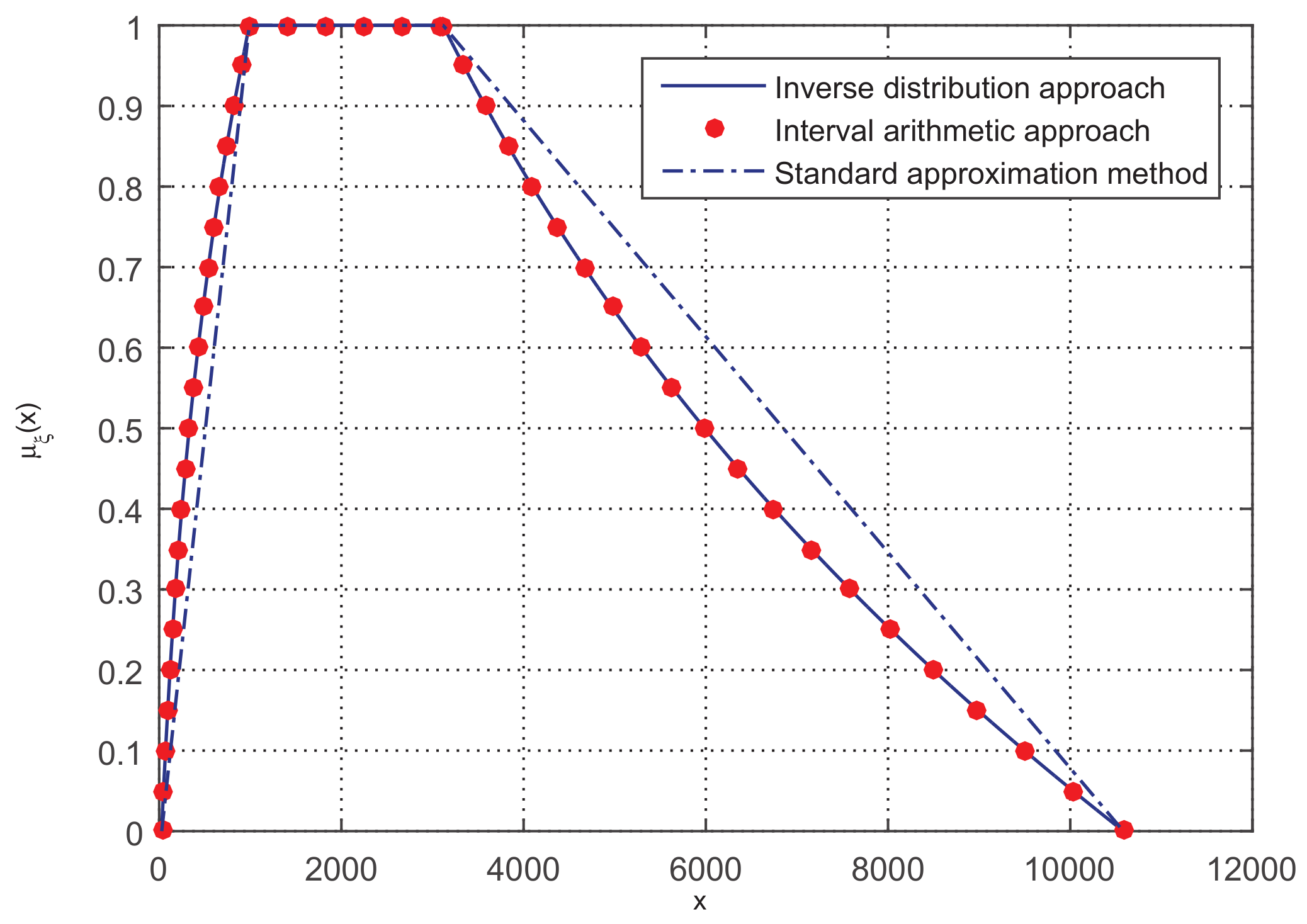
The results of the three approaches are presented in Figure 8, in which “•”, “−”, and “” represent the membership function of the interval arithmetic approach, the inverse credibility distribution approach, and the standard approximation method, respectively. Unsurprisingly, our approach has the same level of accuracy as the interval arithmetic approach, and both of them are much better than the standard approximation method. The aforementioned three examples discuss three different kinds of strictly monotone functions, i.e., strictly increasing, strictly decreasing, and strict monotone, which are widely-used in areas such as forecasting [22,27] and the vehicle routing problem [28]. However, in some situations, the function f involves many ⊗ and ⊙ procedures, which lead to difficulties in acquiring the inverse function of the inverse credibility distribution Ψ of ξ, i.e., the credibility distribution Φ of ξ, and then make the membership function hard to achieve. Owing to the continuity and strict monotonicity of the function f in or , we can obtain its well approximate inverse function by means of the “polyfit’ function in MATLAB to handle the problem, the usage of which is presented in the following example.
Example 8.
Let , , , , and the function . Then, output the membership function of .
The three parameters , , and δ of , , and are , , , and , respectively. Owing to the continuity and strict increase to and and strict decrease to and of the function f, based on Theorem 2, the inverse credibility distribution is
Then, by using the function ‘polyfit’ in Matblab, the credibility distribution can be approximated as
Then, we can obtain the membership function from Theorem 3:
Similarly, Figure 9 represents the membership functions μ of the three approaches. The membership function of the standard approximation method has the worst performance in terms of accuracy and sometimes may have an extremely large error to the exact values. Even though the credibility distribution Φ is approximated by the “polyfit” function in MATLAB, the accuracy of the membership function from our approach can still compete with that obtained by the interval arithmetic approach.
Example 9.
Let , , , , , and the function . Then output the membership function of .
The three parameters , , and δ of , , , , and are , , , , and , respectively. Owing to the continuity and strict increase to , , and and strict decrease to and of the function f, based on Theorem 2, the inverse credibility distribution is
Then, we can obtain the membership function μ of ξ by taking advantage of the function “polyfit” and Theorem 2, and we have the membership function :
The results are illustrated in Figure 10. The function f in this example is much more complex than that in Example 7. However, the result of our approach is satisfying, as before that, it can return almost an exact membership function, whereas the standard approximation approach has a large gap from the other two approaches. From the two examples, it can be clearly seen that the approximate procedures by the “polyfit” function in MATLAB have not much influence on the accuracy of the membership function, no matter whether the function f is simple or complex.
The above five numerical examples range from simple to complex. The functions f of the former three are simple but frequently-used in real applications, and the functions f, containing many ⊗ and ⊙ arithmetic operations, of the last two are much more complex. In simple examples, the membership function resulting from our approach is consistent with that from the interval arithmetic approach, but the superiority of the former approach is the acquisition of the exact membership function. No matter whether the right or the left part of the exporting membership function is considered, the distance from the standard approximation method to the exact value exists and may be extremely large. More details can be seen from the trends of the three approaches’ membership functions represented by the symbols “•”, “−”, and “” in Examples 5 and 6. In the complex examples, although the membership function obtained by inverse credibility distribution approach is approximated in terms of the “polyfit” function in MATLAB, it can still achieve almost the same accuracy as that of the interval arithmetic approach, which can be clearly seen from the result of “•” and `−’ in Figure 9. In brief, compared with the other two approaches, the inverse credibility distribution approach can output not only the exact same membership function as the interval arithmetic approach, but also the expression that the interval arithmetic approach cannot acquire. It should be noted that this is not restricted to the symmetric TFN represented in the aforementioned examples; the inverse credibility distribution approach can apply to all continuous and strictly monotone functions involving regular fuzzy intervals.
5. The Application on a Completion Time Analysis
5.1. The Completion Time Analysis of a Construction Project
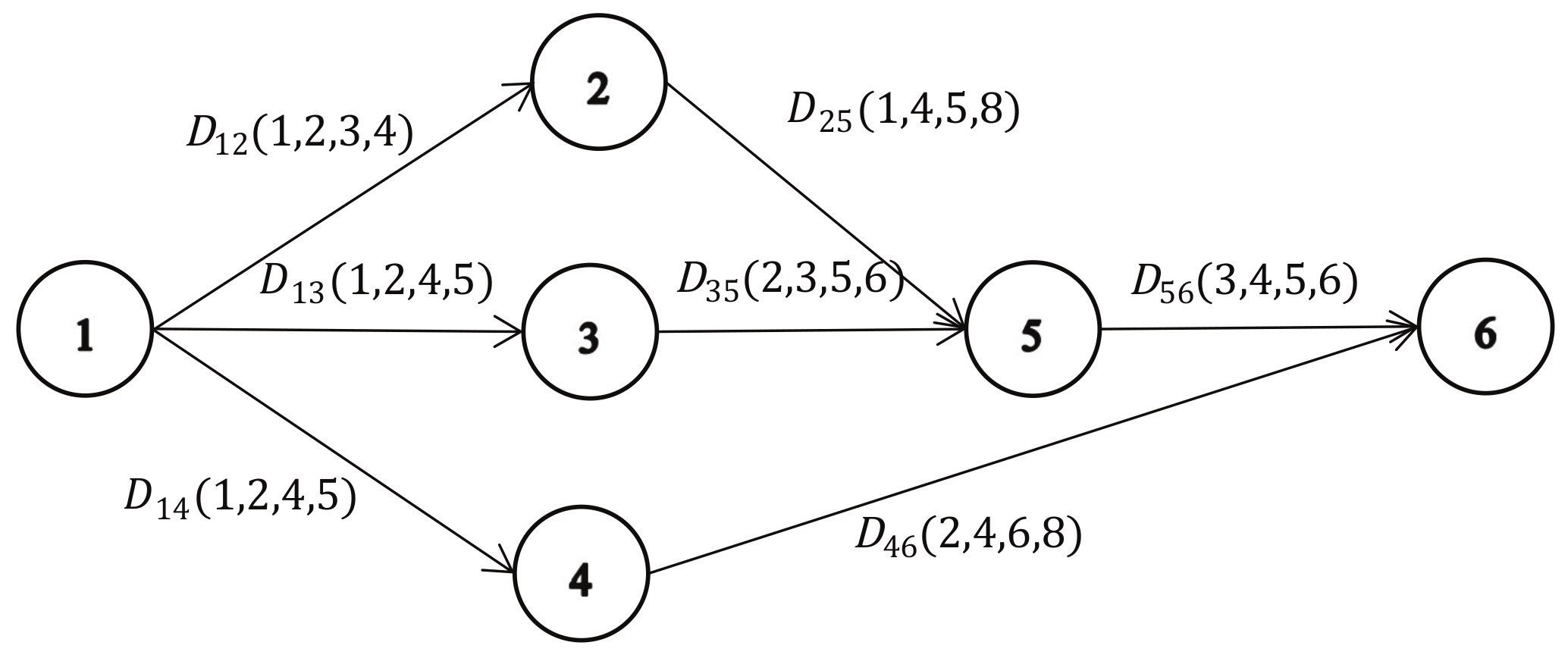
The completion time of a construction project is of great significance in a construction project, since the start and completion time of each activity can only be determined if the completion time is confirmed. In a construction project, various activities, such as material preparation and foundation engineering construction, are included, and those activities have logical dependencies. Scholars and project engineers usually use a project network to describe the relationship in which a pair of nodes with represents the activity and the nodes i and j demonstrate the start and finish node of the activity (see Figure 11, which has six nodes and seven activities). Denote that A is the set of activities in the construction project, and and are the stat and duration time of the activity . We then have the start time of the activity ; that is,
Theoretically speaking, if the node i is larger than all the other nodes, the result of Equation (7) is actually the completion time of the project.
In real applications, the duration time of each activity is not crisp but fuzzy due to the influence of weather and government policy, which creates much more difficulties for the acquisition of the completion time. To tackle this problem, Ke and Liu [18] used a Monte Carlo method-based fuzzy simulation to approximate the membership function of fuzzy completion time, and its main basis is Zadeh’s extension principle [29], which is as follows.
Definition 2.
Let ξ and η be two fuzzy numbers with membership functions and . Then, for a real-valued function f, the membership function μ of is
Denote that is the completion time of the project, is the duration time of the activity with , and f is the function relationship of the activities in Equation (7); we can obtain the completion time, that is, , where . The Monte Carlo method-based fuzzy simulation for the completion time can be designed as follows. Firstly, generate from the -level set of , , where is a sufficiently small number. Suppose that are all the possible values in the set }, apparently with . Based on the operations of and in Equation (8), the membership degree of at , i.e., the membership function of , is estimated by
where is the membership function of the duration of the activity . Generally speaking, if the number N is extremely large, can well approximate the membership function of .
As shown in Equation (8), the relationship function f contains the operations “∨” and “+”, and it can be easily deduced that the function f is continuous and of strict monotonicity from [15], which means that the proposed inverse credibility distribution approach can be used to acquire the membership function of . The following employs a construction project example from Zhao et al. [30] to illustrate the performance of the simulation approach in [18], the inverse credibility distribution approach, and the interval arithmetic approach.
Consider a construction project with six nodes and seven activities (see Figure 11), in which the duration time of each activity is symmetric TFN. From Equation (7), the completion time can be calculated by
Since the function f is continuous and strictly increasing with respect to the duration time , by means of Theorem 1, we can obtain the inverse credibility distribution of as
By taking advantage of Theorems 2–4, the membership function of is
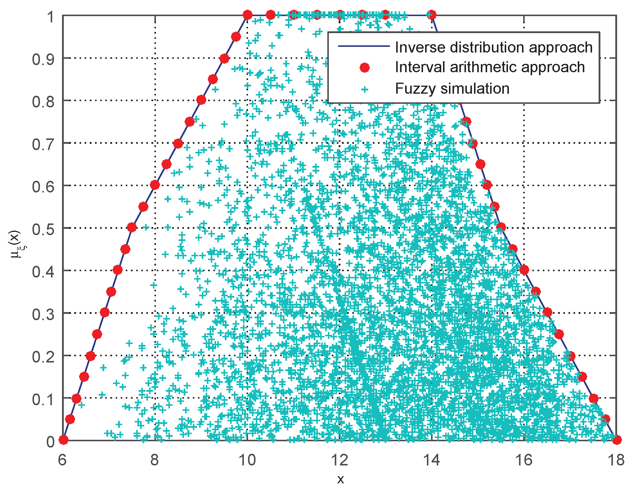
The results of the three approaches are all illustrated in Figure 12, in which the symbols “−”, “•”, and “+” demonstrate the membership function obtained by the inverse credibility distribution approach, the interval arithmetic approach, and the fuzzy simulation [18], respectively.
It should be noted that the standard approximation method cannot apply to the calculation of the completion time, since they have no arithmetic rules in the operations ∨ or ∧. Obviously, the symbol “−” passes through all “•”, which further demonstrates the effectiveness of the inverse credibility distribution approach, in that it can output the accurate membership function not only in numerical examples but also in real applications. Fuzzy simulation performed poorly in terms of accuracy, especially in the domain , and in most cases, the membership function is smaller than the other approaches, which may because of the operations and in Equation (9). The completion time analysis clearly shows the strength of the proposed approach, which is that it can output the exact expression of the membership function, whereas the interval arithmetic approach and fuzzy simulation cannot.
5.2. Comparison Analysis of Proposed Approach with Existing Techniques
The completion time time analysis, together with the aforementioned five examples, gives strong proof for the effectiveness of the proposed approach. To better illustrate the effectiveness of the proposed inverse credibility distribution approach, the performances of the standard approximation method, the interval arithmetic approach, and the fuzzy simulation approach are all summarized in Table 1, where the application area, accuracy, and output expression are employed as the evaluation criteria.
Disappointingly, although the standard approximation method can output the expression of the membership function for functions of fuzzy intervals, its application area is narrow, only for the basic arithmetic operations (i.e., ⊕, ⊖, ⊗, ⊙) with a trapezoidal fuzzy number, and the obtained expression is inaccurate and sometimes has large error (see Example 5 in Section 4). The fuzzy simulation approach can be applied to any functions of fuzzy intervals, but the insufficiency also exists that it cannot output accurate expressions of the membership functions for functions of fuzzy intervals. The application areas of the interval arithmetic approach and the inverse credibility distribution approach are the same, whereas the latter performs even better for the accurate expression of the membership function.
In summary, compared with the other approaches (i.e., the standard approximation method, the interval arithmetic approach, and the fuzzy simulation approach), our approach can output accurate or well-approximated expressions of the membership function of functions involving regular fuzzy intervals, which the others cannot.
6. Conclusions
Our contributions can be summarized in the following three parts: (1) the relationship among the membership function , the credibility distribution , and the inverse credibility distribution of the regular fuzzy interval is proved and summarized in Theorems 2–4. (2) We derive a novel inverse credibility distribution approach for the membership function of the functions of regular fuzzy intervals, i.e., , in which the function f is continuous and of strict monotonicity. (3) Some numerical examples, together with a completion time time analysis, equipping commonly-used symmetric TFNs, are presented to demonstrate the effectiveness of our approach, in which the well-accepted standard approximation method, interval arithmetic approach, and the fuzzy simulation approach are introduced to make a comparison. The comparisons show that the inverse credibility distribution can not only output as accurate a membership function as the interval arithmetic approach but also can acquire the expression of the membership function.
However, it should be noted that although the proposed method is helpful to handle fuzzy arithmetic on functions of regular fuzzy intervals, its application area is only restricted to continuous and strictly monotone functions with regular LR fuzzy intervals. Thus, in the future, we will extend the inverse credibility distribution approach to more general situations, i.e., non-continuous or non-monotone functions regarding other types of fuzzy numbers (such as spherical linear Diophantine fuzzy sets or a circular fuzzy set).
Funding
This work was supported by grants from the Science and Technology Innovative Talents Project of Universities in Henan Province (No. 22HASTIT010), the Fundamental Research Funds for the Universities of Henan Province (No. NSFRF210202), and the Philosophy and Social Science project of Henan Province (No. 2021BJJ043).
Institutional Review Board Statement
Not applicable.
Informed Consent Statement
Not applicable.
Data Availability Statement
Not applicable.
Acknowledgments
The author especially thanks the editors and anonymous referees for their kind review and helpful comments. In addition, the authors would like to acknowledge the gracious support of this work from the Science and Technology Innovative Talents Project of Universities in Henan Province and the Fundamental Research Funds for the Universities of Henan Province.
Conflicts of Interest
We declare that we have no relevant or material financial interests that relate to the research described in this paper. The manuscript has neither been published before, nor has it been submitted for consideration of publication in another journal.
Sample Availability
Samples of the compounds are available from the author.
Abbreviations
The following abbreviations are used in this manuscript:
| STA | Standard approximation method |
| IAA | Interval arithmetic approach |
| ICDA | Inverse credibility distribution approach |
| TFN | Trapezoidal fuzzy number |
| CSM | Continuous and strictly monotone |
| BAO | Basic arithmetic operations |
References
- Zadeh, L.A. Fuzzy sets. Inf. Control 1965, 8, 338–353. [Google Scholar] [CrossRef]
- Riaz, M.; Hashmi, M.R. Linear Diophantine fuzzy set and its applications towards multi-attribute decision-making problems. J. Int. Fuzzy Sys. 2019, 37, 5417–5439. [Google Scholar] [CrossRef]
- Riaz, M.; Hashmi, M.R.; Pamucar, D.; Chu, Y.M. Spherical linear diophantine fuzzy sets with modeling uncertainties in MCDM. CMES-Comp. Model. Eng. 2021, 126, 1125–1164. [Google Scholar] [CrossRef]
- Dubois, D.; Prade, H. Possibility Theory; Plenum Press: New York, NY, USA, 1998. [Google Scholar]
- Dubois, D.; Prade, P. Operations on fuzzy numbers. Int. J. Syst. Sci. 1978, 9, 613–626. [Google Scholar] [CrossRef]
- Giachetti, R.E.; Young, R.E. Analysis of the error in the standard approximation used for multiplication of triangular and trapezoidal fuzzy numbers and the development of a new approximation. Fuzzy Set Syst. 1997, 91, 1–13. [Google Scholar] [CrossRef]
- Guerra, M.L.; Stefanini, L. Approximate fuzzy arithmetic operations using monotonic interpolations. Fuzzy Set Syst. 2005, 150, 5–33. [Google Scholar] [CrossRef]
- Ban, A.I.; Coroianu, L.; Khastan, A. Conditioned weighted L-R approximations of fuzzy numbers. Fuzzy Set Syst. 2016, 283, 56–82. [Google Scholar] [CrossRef]
- Nayagam, V.L.G.; Murugan, J. Hexagonal fuzzy approximation of fuzzy numbers and its applications in MCDM. Complex Intell. Syst. 2021, 7, 1459–1487. [Google Scholar] [CrossRef]
- Hai, S.X. The arithmetic operator of fuzzy regular prismoid numbers and its application to fuzzy risk analysis. Int. J. Comput. Int. Syst. 2021, 14, 1541–1563. [Google Scholar] [CrossRef]
- Kaufmann, A.; Gupta, M.M. Fuzzy Mathematical Models in Engineering and Management Science; Plenum Press: New York, NY, USA, 1988. [Google Scholar]
- Puri, J.; Yadav, S.P. A fuzzy DEA model with undesirable fuzzy outputs and its application to the banking sector in India. Expert. Syst. Appl. 2014, 41, 6419. [Google Scholar] [CrossRef]
- Hatami-Marbini, A. Benchmarking with network DEA in a fuzzy environment. RAIRO-Oper. Res. 2019, 53, 687–703. [Google Scholar] [CrossRef]
- Liu, B.; Liu, Y. Expected value of fuzzy variable and fuzzy expected value models. IEEE Trans. Fuzzy Sys. 2002, 10, 445–450. [Google Scholar]
- Zhou, J.; Yang, F.; Wang, K. Fuzzy arithmetic on LR fuzzy numbers with applications to fuzzy programming. J. Int. Fuzzy Sys. 2016, 30, 71–87. [Google Scholar]
- Xie, X.H.; Liu, Y.Y.; Gu, Y.J.; Zhou, J. Arithmetic operations on triangular fuzzy numbers via credibility measures: An inverse distribution approach. J. Int. Fuzzy Syst. 2018, 35, 3359–3374. [Google Scholar] [CrossRef]
- Zhao, M.X.; Han, Y.L.; Zhou, J. An extensive operational law for monotone functions of LR fuzzy intervals with applications to fuzzy optimization. Technique report. Soft Comput. 2022. Epub ahead of printing. [Google Scholar] [CrossRef]
- Ke, H; Liu, B. Fuzzy project scheduling problem and its hybrid intelligent algorithm. Appl. Math. Model. 2010, 34, 301–308. [Google Scholar] [CrossRef]
- Zhou, J.; Han, Y.; Liu, J.; Pantelous, A.A. New approaches for optimizing standby redundant systems with fuzzy lifetimes. Comput. Ind. Eng. 2018, 123, 263–277. [Google Scholar] [CrossRef]
- Sudakov, V. Improving air transportation by using the fuzzy Origin-Destination matrix. Mathematics 2021, 9, 1236. [Google Scholar] [CrossRef]
- An, M.; Wei, D.J.; Zhang, Y. Fuzzy witness reasoning-based approach to the risk assessment of the deep foundation pit construction. J. Saf. Environ. 2021, 21, 512–520. [Google Scholar]
- Gu, Y.; Zhao, Y.; Zhou, J.; Li, H.; Wang, Y. A fuzzy multiple linear regression model based on meteorological factors for air quality index forecast. J. Int. Fuzzy Syst. 2021, 40, 10523–10547. [Google Scholar] [CrossRef]
- Liu, Y.; Miao, Y.; Pantelous, A.A.; Zhou, J.; Ji, P. On fuzzy simulations for expected values of functions of fuzzy numbers and intervals. IEEE Trans. Fuzzy Syst. 2021, 29, 1446–1459. [Google Scholar] [CrossRef]
- Zadeh, L.A. Fuzzy sets as a basis for a theory of possibility. Fuzzy Set Syst. 1978, 1, 3–28. [Google Scholar] [CrossRef]
- Zadeh, L.A. A theory of approximate reasoning. Mach. Intell. 1979, 9, 149–194. [Google Scholar]
- Liu, B. Theory and Practice of Uncertain Programming; Physica-Verlag Springer: Berlin/Heidelberg, Germany, 2002. [Google Scholar]
- Zhou, J.; Zhang, H.; Gu, Y.; Pantelous, A.A. Affordable levels of house prices using fuzzy linear regression analysis: The case of Shanghai. Soft Comput. 2018, 22, 5407–5418. [Google Scholar] [CrossRef]
- Wang, R.; Zhou, J.; Yi, X.; Pantelous, A.A. Solving the green-fuzzy vehicle routing problem using a revised hybrid intelligent algorithm. J. Ambient. Intell. Humaniz. Comput. 2019, 10, 321–332. [Google Scholar] [CrossRef]
- Zadeh, L.A. The concept of a linguistic variable and its application to approximate reasoning. Inform. Sci. 1975, 8, 199–249. [Google Scholar] [CrossRef]
- Zhao, M.X.; Zhou, J.; Wang, K.; Pantelous, A.A. Project scheduling problem with fuzzy activity durations: A novel operational law based solution framework. Tech. Rep. 2022. under review. [Google Scholar]
Figure 1.
The membership function of a symmetric TFN .

Figure 2.
The credibility distribution of a symmetric TFN .

Figure 3.
Inverse credibility distribution of a symmetric TFN .

Figure 4.
The idea of the inverse credibility distribution approach.

Figure 5.
The flowchart of the inverse credibility distribution approach.

Figure 6.
The membership function of the three approaches in Example 5.

Figure 7.
The membership function of the three approaches in Example 6.

Figure 8.
The membership function of the three approaches in Example 7.

Figure 9.
The membership function of the three approaches in Example 8.

Figure 10.
The membership function of the three approaches in Example 9.

Figure 11.
A construction project with six nodes and seven activities.

Figure 12.
The membership function of the completion time [29].
Figure 12.
The membership function of the completion time [29].


Table 1.
The comparisons of the four approaches.
| No. | Name | Application Area | Accuracy | Output Expression | |||
|---|---|---|---|---|---|---|---|
| Function f | Fuzzy Interval | Accurate | Approximate | Yes | No | ||
| 1 | STA | BAO | TFN | √ | √ | ||
| 2 | IAA | CSM | Regular | √ | √ | ||
| 3 | ICDA | CSM | Regular | √ | √ | ||
| 4 | FS [18] | All | All | √ | √ | ||
STA: standard approximation method, IAA: interval arithmetic approach, FS: fuzzy simulation, ICDA: inverse credibility distribution approach, TFN: trapezoidal fuzzy number, CSM: continuous and strictly monotone, BAO: basic arithmetic operations.
Publisher’s Note: MDPI stays neutral with regard to jurisdictional claims in published maps and institutional affiliations. |
© 2022 by the author. Licensee MDPI, Basel, Switzerland. This article is an open access article distributed under the terms and conditions of the Creative Commons Attribution (CC BY) license (https://creativecommons.org/licenses/by/4.0/).
Share and Cite
MDPI and ACS Style
Gu, Y. A Novel Inverse Credibility Distribution Approach for the Membership Functions of LR Fuzzy Intervals: A Case Study on a Completion Time Analysis. Symmetry 2022, 14, 1554. https://0-doi-org.brum.beds.ac.uk/10.3390/sym14081554
AMA Style
Gu Y. A Novel Inverse Credibility Distribution Approach for the Membership Functions of LR Fuzzy Intervals: A Case Study on a Completion Time Analysis. Symmetry. 2022; 14(8):1554. https://0-doi-org.brum.beds.ac.uk/10.3390/sym14081554
Chicago/Turabian StyleGu, Yujie. 2022. "A Novel Inverse Credibility Distribution Approach for the Membership Functions of LR Fuzzy Intervals: A Case Study on a Completion Time Analysis" Symmetry 14, no. 8: 1554. https://0-doi-org.brum.beds.ac.uk/10.3390/sym14081554
Note that from the first issue of 2016, this journal uses article numbers instead of page numbers. See further details here.