
Uncertainty Theory-Based Resilience Analysis for LEO Satellite Communication Systems


1
School of Reliability and Systems Engineering, Beihang University, Beijing 100191, China
2
Science and Technology on Reliability and Environmental Engineering Laboratory, Beijing 100191, China
3
School of Aeronautic Science and Engineering, Beihang University, Beijing 100191, China
4
Institute of Telecommunication and Navigation Satellites, China Academy of Space Technology, Beijing 100094, China
*
Author to whom correspondence should be addressed.
Symmetry 2022, 14(8), 1568; https://0-doi-org.brum.beds.ac.uk/10.3390/sym14081568
Submission received: 5 July 2022
/
Revised: 25 July 2022
/
Accepted: 26 July 2022
/
Published: 29 July 2022
(This article belongs to the Special Issue Uncertainty Theory: Symmetry and Applications)
Abstract
:Resilience, the ability of a system to withstand disruptions and quickly return to a normal state, is essential for a low-Earth-orbit satellite communication system (LEO-SCS), as its large number of satellites, may encounter various disturbances. As a developing system with asymmetrical and insufficient data, it is with both aleatory and epistemic uncertainties, which renders existing resilience measures inapplicable. This paper utilizes uncertainty theory to define belief instantaneous availability, based on which a new resilience measure for the LEO-SCS is proposed. As the resilience is mainly determined by the dynamic and uncertain characteristics of an LEO-SCS, an uncertain satellite network evolution model is developed to describe its operating patterns, and an evaluation method is proposed to estimate its resilience. To illustrate our proposed uncertain theory-based resilience evaluation method, an LEO-SCS case with 48 satellites is studied, and its resilience values under different backup strategies are compared to assist in system design decisions.
1. Introduction
Due to short round-trip delays and wide-area coverage, the low-Earth-orbit satellite communication system (LEO-SCS) is becoming an important research topic. Iridium NEXT, OneWeb, and StarLink are typical examples. During system operation, disruptions may occur, causing satellite failure or signal interruption. The failure to quickly and effectively solve these problems may lead to huge economic losses. How to reasonably quantify and evaluate the impact of these failures is important to improve LEO-SCS operation and service stability.
As an extension and expansion of reliability and risk, resilience is the ability of a system to withstand disruption and quickly return to a normal state. Resilience, which encompasses avoidance, robustness, reconstitution, and recovery, has become a key criterion in evaluating alternative space systems, including constellations [1,2]. Researchers have already analyzed the resilience of constellation systems. Turner [3] defined the resilience of a satellite network as the time-averaged network performance under an extreme-event situation and built an extreme event model to quantify the resilience of satellite communication systems. Han et al. [4] proposed a three-dimensional resilience evaluation matrix and analyzed the resilience of a communication constellation based on the coverage capacity and reconstruction energy index. Lowe and Macdonald [5] used a Markov chain and semi-analytical approach to assess the resilience of both networking- and non-networking-capable constellation systems. Researchers have also proposed resilience assessment methods for other networked systems. Reed et al. [6] defined resilience as the ratio of the integral of the performance function to the recovery time. Ouyang et al. [7] defined it as the ratio of the real performance integral to the target one during a year. Li et al. [8] defined resilience as the average performance within the maximum allowable recovery time. Moutsinas et al. [9] developed a resilience measure based on the polynomial chaos expansion method, which could characterize the resilience for a wide range of uncertainty distributions.
It is important to analyze resilience during the design of a system, as it can guide resilience design and provide reasonable strategies. However, current resilience measures and modeling methods cannot be directly applied to the LEO-SCS design process for the following reasons:
- Generally, there are two types of uncertainties, aleatory and epistemic. Epistemic uncertainties can be reduced by collecting more data or refining models, and aleatory ones are natural randomness that cannot be reduced [10]. As a typical newly developing system, the LEO-SCS suffers from performance data insufficiency and performance data asymmetry [11], which limits knowledge on recognizing system performance and leads to epistemic uncertainty. Considering the aleatory uncertainty of the satellite failures [12] and the epistemic uncertainty of the system performance, the resilience of an LEO-SCS needs to be analyzed with both uncertainties. However, existing resilience assessment methods only individually focus on either aleatory uncertainty or epistemic uncertainty [3,4,5,13], which will lead to inaccurate resilience assessment. In addition, the performance measures used in these resilience assessments vary widely and a unified measure is required for the resilience comparison among different systems.
- To measure LEO-SCS resilience requires a system model to be built. Previous LEO-SCS modeling methods have only considered the dynamics of the network topology and the aleatory uncertainty of the performance parameters while neglecting their epistemic uncertainty.
The uncertainty theory, founded by Liu [14], defines uncertain measures to quantify events with epistemic uncertainty. Then, Liu [15] extended the uncertain measure to chance measure for events with both aleatory and epistemic uncertainties. According to the above research, we propose a new resilience measure and modeling method for LEO-SCS based on uncertainty theory. Our contributions are as follows:
- An uncertain satellite network evolution model is proposed for the LEO-SCS, which quantifies both the end-to-end aleatory and epistemic uncertainties and also considers dynamic topology changes;
- A resilience evaluation method is proposed for the LEO-SCS, under which system resilience under different backup strategies can be compared and the results can be used in design decisions.
The remainder of this paper is organized as follows. Section 2 briefly introduces uncertainty and chance measures. A belief resilience measure is proposed in Section 3. Section 4 introduces the LEO-SCS and provides an uncertain satellite network evolution model for it. A resilience evaluation method for the LEO-SCS is presented in Section 5. Section 6 illustrates the effectiveness of our proposed methodology through a specific case and discusses the impact of different backup strategies on system resilience. Concluding remarks are provided in Section 7.
2. Preliminaries
In this section, we introduce some important concepts of the uncertainty and chance measures.
2.1. Uncertain Measure
Definition 1
(Liu [14]). Uncertain measure is a real-valued set-function on a σ-algebra over a nonempty set Γ that satisfies the following four axioms:
Axiom 1: (Normality Axiom) for the universal set Γ.
Axiom 2: (Duality Axiom) for any event Λ.
Axiom 3:(Subadditivity Axiom) For every countable sequence of events , we have
Axiom 4: (Product Axiom) Let be uncertainty spaces for . The product uncertain measure is an uncertain measure satisfying
where are arbitrarily chosen events from for , respectively.
Definition 2
(Liu [14]). An uncertain variable is a function ξ from an uncertainty space to the set of real numbers such that is an event for any Borel set B of real numbers.
Definition 3
(Liu [14]). The uncertainty distribution Φ of an uncertain variable ξ is defined by for any real number x.
Example 1
(Liu [14]). An uncertain variable ξ is called a linear variable if it has a linear uncertainty distribution
denoted by , where a and b are real numbers with .
Example 2
(Liu [14]). An uncertain variable ξ is called a zigzag variable if it has a zigzag uncertainty distribution
denoted by , where a, b and c are real numbers with .
Definition 4
(Liu [16]). An uncertainty distribution Φ is said to be regular if its inverse function exists and is unique for each .
Theorem 1
(Liu [16]). Let be independent uncertain variables with regular uncertainty distributions , respectively. If f is a strictly increasing function, then has an inverse uncertainty distribution .
2.2. Chance Measure
The chance measure [15] combines probability and uncertain measures to solve problems with both aleatory and epistemic uncertainties. Its concepts, as used in this article, are as follows.
Let be a uncertainty space and be a probability space. Then the is called a chance space.
Definition 5
Definition 6
3. Belief Resilience Measure
We present a new belief resilience measure to overcome the limitations of the commonly used resilience measures introduced in Section 1.
3.1. Belief Instantaneous Availability
Instantaneous availability is the probability that a system or component is performing its required function (i.e., required performance) at a given point in time [17], and it can reflect the overall situation of the system or component. We apply this parameter as the basis for the resilience measure. Considering that the system performance parameters are affected by aleatory and epistemic uncertainties, the belief instantaneous availability is defined based on the uncertainty theory [14,15] as follows.
Definition 8.
Belief instantaneous availability is the chance that the system performance margin is greater than 0 at time t, i.e.,
where
where STB, LTB, and NTB, respectively, are the smaller-the-better, the larger-the-better, and the nominal-the-better parameters, and [18] describes the distance between a performance parameter and its failure threshold at time t. If , a failure occurs, and means the system is within the available zone that can be operated at time t.
If a performance parameter is mainly with aleatory uncertainties, the performance margin degenerates to a random variable. Let denote the belief instantaneous availability under the probability theory and we have
If a performance parameter is mainly with epistemic uncertainties, the performance margin degenerates to an uncertain variable. Let denote the belief instantaneous availability under the uncertainty theory and we have
3.2. Belief Resilience
Definition 9.
The belief resilience of a system with epistemic and aleatory uncertainties is the chance that it can withstand disruption and recover quickly.
Define as an uncertain random variable that describes a system’s behavior after a disruption, with feasible domain . The belief resilience can be measured as
If is a random variable, we have . If is an uncertain variable, we have .
We focus on the belief instantaneous availability change after a disruption, and the belief resilience can be defined as
where is the time when a disruption occurs; is the maximum allowable recovery time determined by users; and are, respectively, the belief instantaneous availability under a specific disruption d and in the normal state (without disruption); and is the requirement for the system’s behavior after a disruption.
Based on Definition 8, the belief instantaneous availability under a specific disruption and normal state (without disruption), respectively, can be calculated as
where and are respective performance margins under specific disruption d and in the normal state (without disruption).
4. LEO-SCS and Its Uncertain Evolution Model
4.1. A Short Introduction to LEO-SCS
An LEO-SCS is composed of LEO satellites, user segments, and gateways [19], see Figure 1. The user segment includes various user terminals, such as fixed terminals, handheld devices, and vehicle-based and airborne terminals. The gateway is a ground station that transmits data between the satellite and terrestrial networks. Links between LEO satellites are inter-satellite links (ISLs), links between LEO satellites and user terminals are user links (ULs), and links between LEO satellites and the gateways are feeder links (FLs).
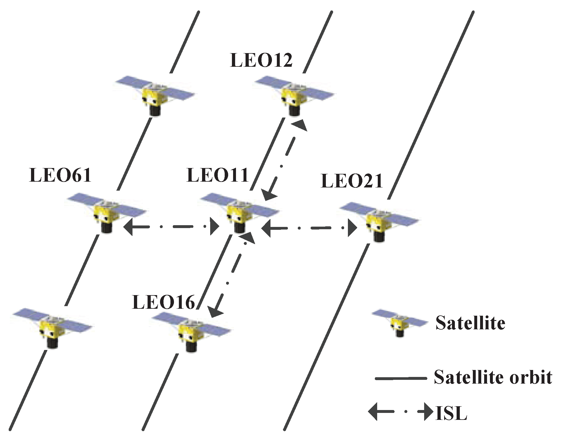
There are both intra-plane and inter-plane ISLs. For example, each satellite in Figure 2 has four adjacent ISLs. In this figure, LEO12, LEO16, and LEO11 are in the same orbit plane, and between them are intra-plane ISLs. LEO61, LEO21, and LEO11 are in different orbit planes, and between them are inter-plane ISLs.
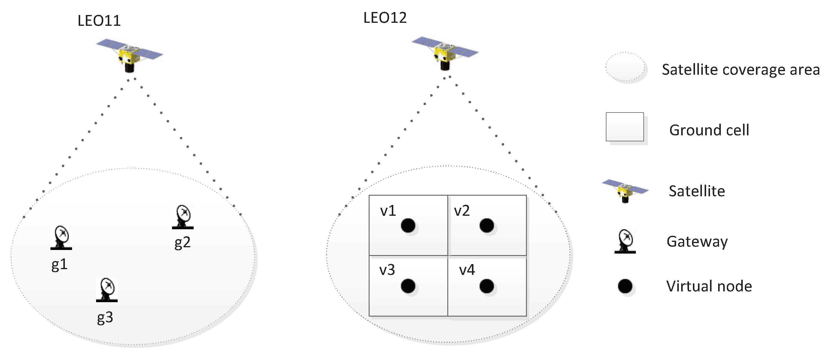
As the number of user terminals is quite large, the Earth’s surface is divided into grids of equal area, and each uses a virtual node (VN) [20,21] to provide services for all user terminals in the grid. Messages are transmitted between the VN and the satellite node through the UL. In an LEO-SCS, ULs and FLs can be built between satellites and connectable gateways/VNs according to the access criteria. A connectable gateway/VN of a satellite is located within its coverage area. In Figure 3, , , and are connectable gateways of LEO11, and , , , and are connectable VNs of LEO12. A satellite connects to a specific gateway/VN according to an access criterion. Access criteria for an LEO-SCS include load balancing, minimum delay, maximum service time, strongest signal, and maximum available channels [22,23].
There are two types of communication methods in LEO-SCS [24]:
- Between user terminals: user terminals can connect directly with an LEO satellite, and the messages are transmitted through one or more LEO satellites from the source to the destination;
- Between user terminal and terrestrial users: a terrestrial user can only connect with its gateway; the gateway and user terminal transfer messages through one or more LEO satellites.
4.2. Uncertain Satellite Network Evolution Model
4.2.1. Assumptions
We build the uncertain satellite network evolution model based on the following assumptions:
- User terminals and gateways are perfect, and only satellite failures, which are affected by aleatory uncertainty [12], are considered, as maintenance is not easy in space;
- Processing delays of an LEO-SCS follow regular uncertainty distributions.
4.2.2. Uncertain Satellite Network Evolution Modeling Method
Considering that only limited performance data (e.g., processing delays) can be obtained in an LEO-SCS, the system has the following three characteristics:
To the best of our knowledge, no researcher has simultaneously considered all three of these characteristics in LEO-SCS modeling. Therefore, we propose an uncertain satellite network evolution modeling method, using a dynamic, uncertain satellite network model to characterize the epistemic uncertainty of satellite performance (i.e., the processing delay) and topology dynamics and applying the evolution rule of the dynamic, uncertain satellite network model to describe the topology evolution process of an LEO-SCS with satellite failures and recoveries.
4.2.3. Dynamic Uncertain Satellite Network Model
Definition 10.
A network is a dynamic uncertain network if its topology changes with time, and the weights of its edges are uncertain variables that vary with time.
A dynamic uncertain network can be denoted as , where V is the node set, is the edge set that varies over time, and is the weight set composed of uncertain variables that vary with time, which can be the cost, distance, or capacity of edges.
In an LEO-SCS, the end-to-end delay, which depends on the propagation delay and processing delay [22], is the key performance parameter [28,29,30,31]. Propagation delay is the time used by electromagnetic waves to transmit a certain distance and it depends on the lengths of links (i.e., ISLs, ULs, and FLs). Processing delay is the time required for nodes (i.e., satellites, user terminals, and gateways) to check the frame’s header and determine where to forward the frame. In an LEO-SCS, since the lengths of links periodically change with time, the propagation delay is a deterministic variable that varies with time. However, because limited data on processing delays can be obtained before LEO-SCS deployment, the processing delay has epistemic uncertainty. So, the end-to-end delay of an LEO-SCS is an uncertain variable that varies with time.
To describe an LEO-SCS in the normal state, a dynamic uncertain satellite network model can be built, where is the node collection of satellites, gateways, and VNs; is the edge collection of ISLs, ULs, and FLs; and is the delay of edges. Using this model, both the dynamics of network topology and the epistemic uncertainty of performance parameters can be expressed. Here, we use an LEO-SCS dynamic adjacency matrix to represent the dynamic, uncertain satellite network model, and it can be divided into an inter-satellite adjacency matrix , a satellite-gateway adjacency matrix , and a satellite-VN adjacency matrix according to the types of links. The LEO-SCS dynamic adjacency matrix is
where X, Y, and Z are the numbers of satellites, gateways, and VNs, respectively, in the system. We describe , , and in Table 1.
Faced with insufficient data, uncertainty statistics methods can be used to obtain the uncertainty distributions of processing delay on the satellite, gateway, and VN.
4.2.4. Evolution Rule of Dynamic Uncertain Satellite Network Model
The dynamic uncertain satellite network model describes the operation of an LEO-SCS in the normal state. However, in the actual operation, the satellite network is evolving due to the failure and recovery of satellites.
Definition 11.
The topology evolution of an LEO-SCS is the topology change of the system caused by satellite entry and exit due to its failure and recovery.
We present the evolution rule of the dynamic, uncertain satellite network model, including timing and an algorithm, to describe the topology evolution of the network structure.
- (1)
- Evolution timing
According to Definition 11, the topology evolution of the satellite network is caused by satellite failure and recovery. Once a satellite fails, it will de-orbit and a backup satellite will be transferred to the site of failure. The evolution timing of the system is as follows:
- Node exit time depends on the satellite failure time;
- (2)
- Evolution algorithm
To model the uncertain satellite network evolution model, satellite failures and recoveries are added to the dynamic, uncertain satellite network model. The evolution algorithm is summarized as Algorithm 1, whose symbols are explained in Table 3.
Using Algorithm 1, can be obtained by: (a) deleting the node and all its adjacent edges when it exits; and (b) adding the node and corresponding edges back when it enters.
| Algorithm 1 Evolution algorithm |
|
5. Resilience Evaluation for the LEO-SCS
To evaluate the resilience of an LEO-SCS, the end-to-end delay calculation method is presented. Then, the belief instantaneous availability can be computed, and the resilience of the LEO-SCS can be evaluated.
5.1. End-to-End Delay Calculation
Using a virtual topology strategy [34,35], the operation time of an LEO-SCS can be divided into discrete time slices with interval . When is small enough, the topology can be considered static in each time slice. Therefore, the uncertain satellite network evolution model can be divided into multiple static uncertain networks with time interval , and the static uncertain network at the kth time slice can be denoted as . Then, the end-to-end delay can be calculated on each static uncertain network.
In an LEO-SCS, applications generally choose the delay minimization path for transmission. We use the most shortest path algorithm (Gao. [36]) to find such a path and calculate the end-to-end delay in the uncertain satellite network evolution model. Using this algorithm, an uncertain programming model is built to select the path that satisfies the maximum allowable delay (i.e., the delay threshold) with the maximum belief degree,
where is the belief degree at the kth time slice, is any path from the source node to the destination node at the kth time slice, is the delay on edge , and is the delay threshold of the application.
Using an uncertain programming model, the delay minimization path with the maximum belief degree can be obtained for the static uncertain network, and the uncertain distribution of the end-to-end delay on the delay minimization path can be calculated. For details, please refer to Gao [36].
5.2. Belief Instantaneous Availability Calculation
The belief instantaneous availability can be computed from the uncertain distribution of the end-to-end delay calculated above. For an LEO-SCS, the service requirement differs by application, and the belief instantaneous availability should be computed separately.
As mentioned in Section 4, we use the end-to-end delay (an STB parameter) as the key performance parameter for LEO-SCS. The belief instantaneous availability for application i under a specific disruption and that under a normal state (without disruption) are influenced by epistemic uncertainties and can be respectively computed as
and
where is the delay threshold of application i, and are its end-to-end delay under one specific disruption and normal state at time t, respectively, and and are the delay margin of application i in one specific disruption and normal state at time t, respectively.
Considering the traffic volume of each application, the belief instantaneous availability of an LEO-SCS under one specific disruption and its normal state can be calculated as
respectively, where is the number of applications in the system, and is the traffic volume of application i at time t. Combining Equations (11) and (15)–(17), the resilience of an LEO-SCS can be computed.
5.3. Resilience Evaluation
Using the belief instantaneous availability calculation method, the resilience of an LEO-SCS can be evaluated as follows:
- Gather the information of applications on the system, including traffic volume , source node, destination node, and delay threshold ;
- Use the uncertain satellite network evolution model in Section 4.2 and the delay bounded routing algorithm in Section 5.1 to simulate the end-to-end delay of each application for every time interval under a specific disruption (i.e., with satellite failure) and in a normal state (i.e., without satellite failure);
- Repeat steps (2) and (3) N times, and calculate that there are behaviors after a disruption that are greater than . The belief resilience of the LEO-SCS is
6. Case Study
6.1. Overview
6.1.1. Topology
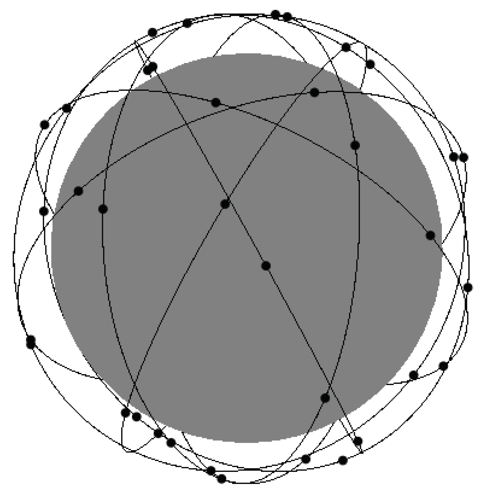
We consider a Walker LEO-SCS with eight orbital planes at a height of 1300 km. The inclination of each orbital plane is 70 degrees, and six satellites are evenly distributed on each plane. As shown in Figure 4, each satellite has four adjacent satellites, two intra-planes and two inter-planes.
There are four gateways in the system-in Beijing, Haikou, Kashgar, and Jiamusi. These connect the terrestrial network in China with the satellite network, and all can provide satellite connections for terrestrial users.
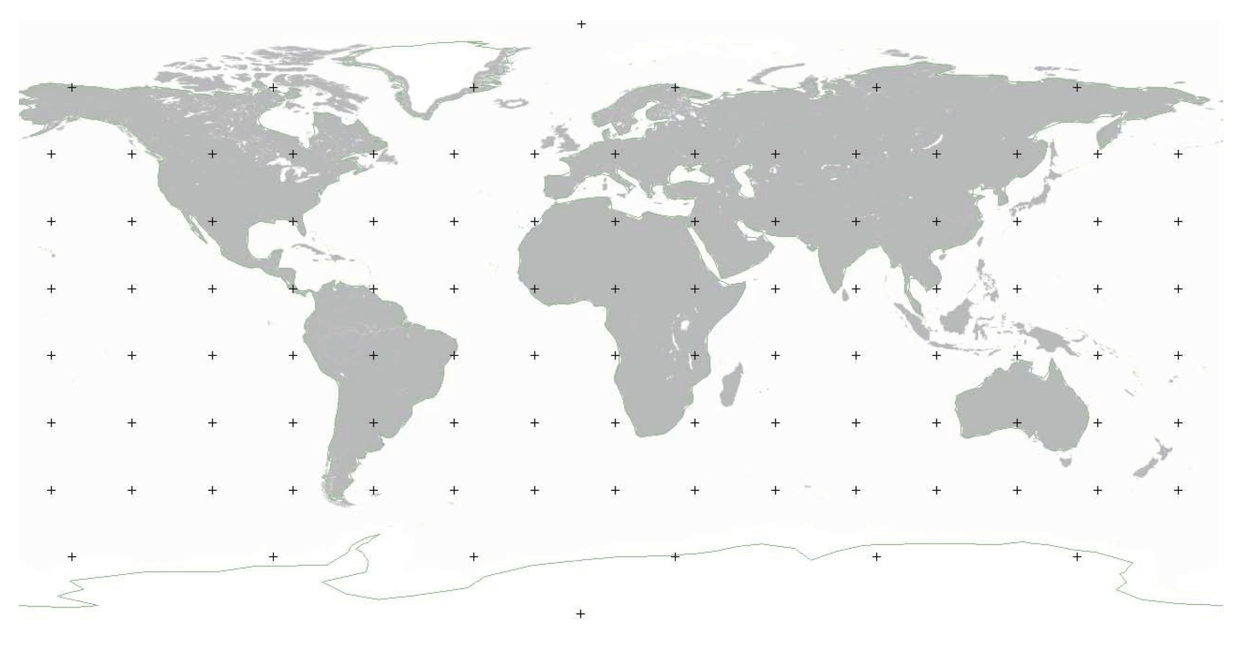
According to the virtual node strategy in Section 4.1, we divide the Earth’s surface into 104 ground grids, each with an area of about square kilometers. A virtual node is set at the center of each grid, to provide service for all terminal users in the grid. Figure 5 shows the 104 virtual nodes, which are marked with plus (‘+’) signs.
As described in Section 4.2.1, the processing delay of each node in the system is considered an uncertain variable. To the best of our knowledge, processing delay of communication networks has not yet been characterized as uncertain variables. When the delay is a random variable, it can be represented by the uniform distribution [37,38]. Considering that the delay in an LEO-SCS depends on the propagation delay and processing delay and the latter one is a deterministic variable, we assume that the processing delays of satellites and virtual nodes obey a linear uncertainty distribution, the processing delays of gateways follow a zigzag uncertainty distribution, and their related parameters are shown in Table 4.
6.1.2. Application
We consider transmissions between user terminals and terrestrial users in China, where all applications have the same priority. The delay bounded routing algorithm in Section 5.2 is used, and the delay thresholds of all applications are 200 ms.
The traffic requirement from zone to zone at hour H can be calculated as [39]
where is the user density in , is the host density in , is the distance between and , is the activity percentage at hour H in .
6.1.3. Failure and Recovery
We assume that the failure time of satellites in an LEO-SCS are independently and identically distributed with an exponential distribution, with a failure rate of , where years is the design lifetime of satellites.
The in-orbit and ground backup strategies in Section 4.2.4 are designed for an LEO-SCS as follows.
- In-orbit backup strategy: each operating orbit has a backup orbit that locates directly below at a height of 1000 km, and one backup satellite is deployed in each backup orbit;
- Ground backup strategy: each launch can carry one backup satellite to supplement the in-orbit backup, and the ground transfer time obeys a uniform distribution, days.
The maximum allowable recovery time of the system is determined as 15 days.
6.2. Resilience Analysis and Discussion
We built the uncertain satellite network evolution model for this Walker LEO-SCS according to Section 4.2, and the system resilience is computed according to the resilience estimation model in Section 5.
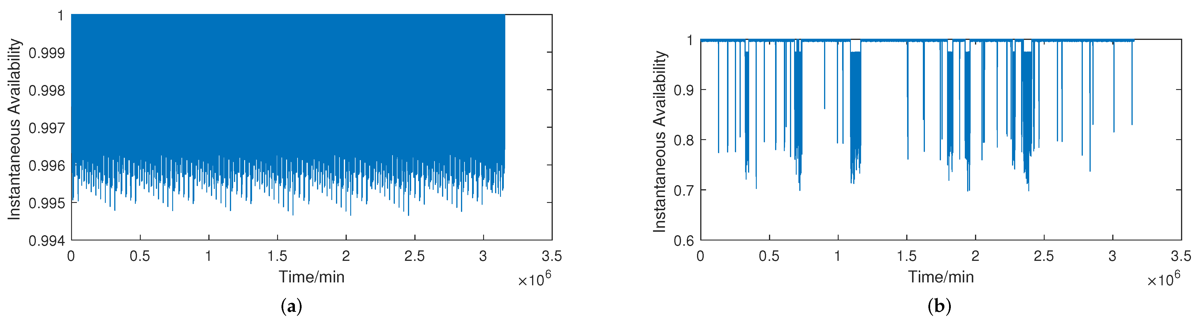
Figure 6 shows the belief instantaneous availability of LEO-SCS under both ideal and actual conditions over 6 years. As shown in Figure 6a, the belief instantaneous availability of the system fluctuates in the range of . Fluctuation is caused by the dynamic movement of the satellites and internet traffic intensity changes over time. From Figure 6b, one can see that the belief instantaneous availability of the system degrades several times under actual conditions, and these are caused by satellite failure.
When a satellite fails, the link connected with it also fails, the network topology of the system evolves, and ground nodes previously connected through the failed satellite must find another connectable satellite. If none exists, the ground node will lose the satellite connection. Transmissions previously relayed through the failed satellite must select a new path. As the LEO-SCS applies the delay bounded routing algorithm, the new connection or path tends to be longer than the original at the same belief degree. So, satellite failure will cause delay-based availability to decrease, and instantaneous availability will fluctuate at a lower level until a backup satellite replaces the failed one. From Figure 6b, it can be seen that: (1) some degradations recover quickly and some slowly, depending on whether the in-orbit backup can be used when the satellite fails; (2) availability degradation varies due to the number of satellite failures and the failure time. Two examples are used to illustrate these phenomena.
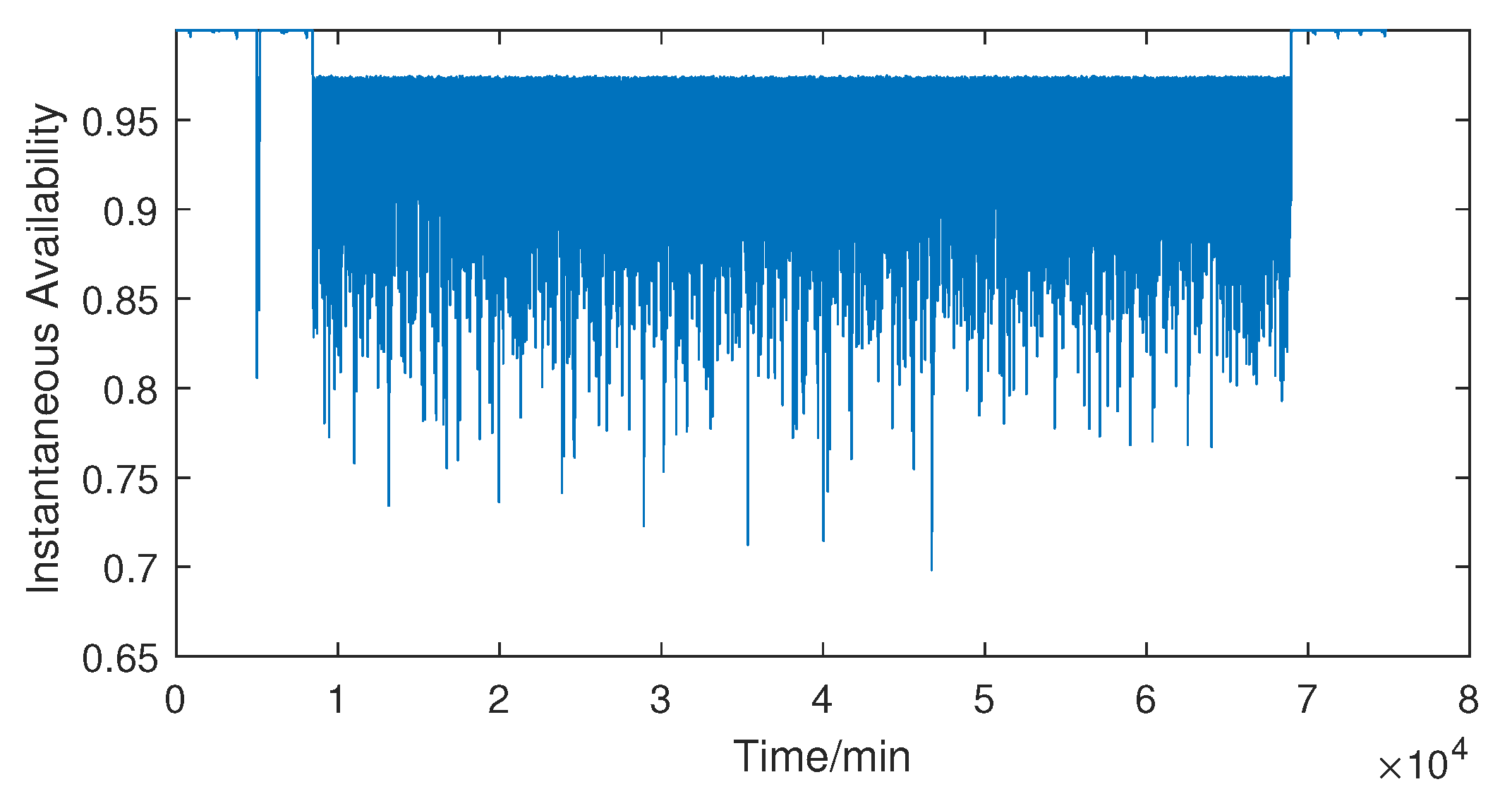
Figure 7 shows the belief instantaneous availability of a system when two co-orbiting satellites fail successively. At time min, the first satellite failed, and the system was restored after 193 min using its in-orbit backup. At time min, another satellite in the same orbit failed. The only in-orbit backup was used when the first satellite failed, there was no in-orbit backup when the second satellite failed, and the system had to wait for a ground backup. Therefore, the second system recovery consumed a much longer time, and the system was restored at time t = 68,952 min.
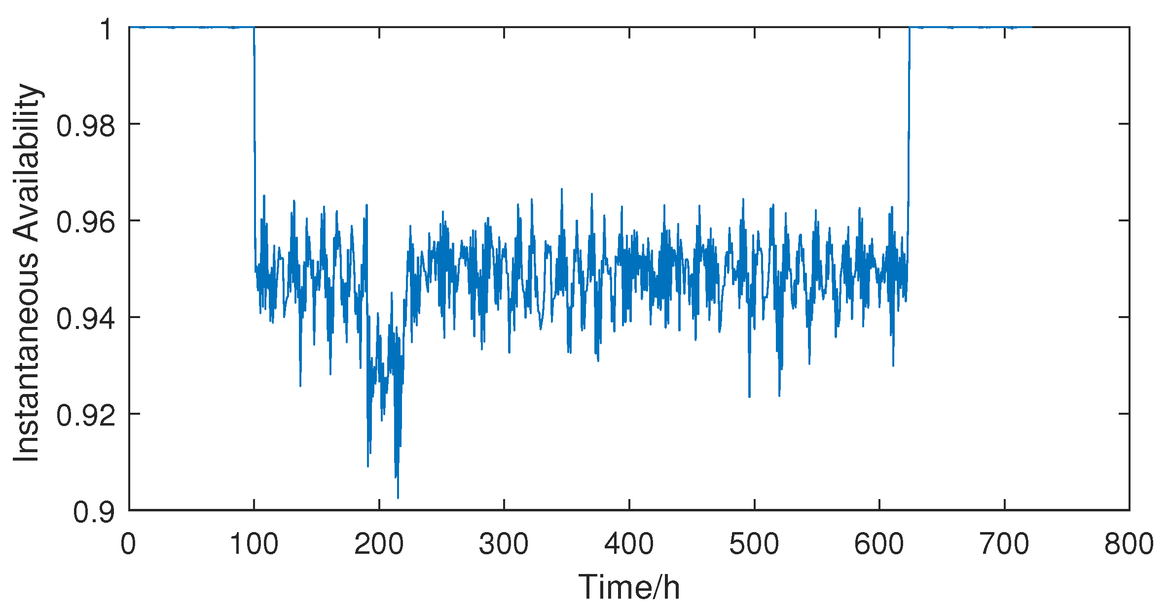
Figure 8 shows the belief instantaneous availability of a system under dual satellite failures. The first satellite failed at time h, which slightly reduced the system availability. At time h, another satellite failed in another orbit, but the first failed satellite was not recovered, as its in-orbit backup had been consumed earlier. At this time, two satellites in the system failed. Compared with a single satellite failure, more ground nodes lose satellite connectivity, and more users choose new longer paths in this case. This led to further availability degradation. When the second failed satellite was recovered using its in-orbit backup at time h, the system availability increased to the level under the single satellite failure. At time h, the first failed satellite was recovered using the ground backup, and the system availability returned to the normal.
In the case above, the backup strategies included both in-orbit and ground backup. When dual satellite failures occur, the possibility that different recovery strategies are adopted, as shown in Table 5. The number of in-orbit backups in each orbit is 1. One can see that over 90% of dual satellite failures use at least one ground backup. Ground backup takes longer to restore the system, and during this time, other satellites are more likely to fail. Therefore, the probability of dual satellite failures can be reduced by increasing the number of in-orbit backups and decreasing the transfer time of the ground backup. Using this method, system resilience can be improved.
According to the analysis above, the satellite recovery time significantly affects the system belief instantaneous availability and thus the system resilience. In an LEO-SCS, the number of in-orbit backups and the satellite orbital lifetime determine the recovery time in practice. We calculated the system resilience under different satellite compositions and backup strategies when the requirement for the system’s behavior after a disruption was 0.99. The results are shown in Table 6.
As shown in Table 6, adding more in-orbit backups and extending satellite orbital lifetimes can improve the resilience of an LEO-SCS because more in-orbit backup reduces satellite recovery time and a longer satellite orbital lifetime reduces the probability of satellite failure. The initial increment on in-orbit backups is more effective than subsequent ones. For example, when the number of in-orbit backups increases from 1 to 2, the system resilience increases more than when backups increase from 2 to 3. Therefore, when designing an in-orbit backup strategy for an LEO-SCS, it is necessary to consider satellite orbital lifetimes, system resilience, and cost comprehensively.
7. Conclusions
We proposed a belief resilience measure. Based on this, a dynamic uncertain satellite network evolution model was developed to describe a dynamic uncertain LEO-SCS, and a methodology was proposed to estimate the resilience of the model. A Walker LEO-SCS with 48 satellites was used to demonstrate the effectiveness of our method, and the influence of the number of in-orbit backups and the satellite orbital lifetime on system resilience was analyzed. The results show that the proposed measure can be used to quantify the resilience of systems with aleatory and epistemic uncertainties. The recovery time of satellites is the main factor affecting system resilience, and the number of in-orbit backup satellites and the satellite orbital lifetime play important roles in increasing LEO-SCS resilience. The proposed resilience evaluation methodology can be used for LEO-SCS comparison, optimization, and design.
The number of satellites in an LEO-SCS has reached hundreds or thousands. How to quickly and accurately assess the resilience of such giant systems will be studied further in our future research.
Author Contributions
Conceptualization, J.M. and R.K.; methodology, J.M.; software, J.M.; validation, J.M. and R.L.; formal analysis, J.M., R.L. and Q.Z.; investigation, J.M. and R.L.; resources, L.L. and X.W.; writing—original draft preparation, J.M.; writing—review and editing, J.M., R.L., R.K. and Q.Z.; supervision, R.L. and R.K.; project administration, R.L. and R.K.; funding acquisition, R.L. and R.K. All authors have read and agreed to the published version of the manuscript.
Funding
This research was funded by the National Natural Science Foundation of China (61773044) and the National Key Laboratory of Science and Technology on Reliability and Environmental Engineering (WDZC2019601A301,6142004210102), and National Natural Science Foundation of China (62073009).
Institutional Review Board Statement
Not applicable.
Informed Consent Statement
Not applicable.
Data Availability Statement
Not applicable.
Conflicts of Interest
The authors declare no conflict of interest.
References
- Schrogl, K.U. Handbook of Space Security: Policies, Applications and Programs; Springer: Berlin/Heidelberg, Germany, 2019. [Google Scholar]
- DOD. FACT SHEET: Resilience of Space Capabilities; Technical Report; Department of Defence: Canberra, ACT, Australia, 2011. [Google Scholar]
- Turner, J.S. A Methodology for Measuring Resilience in a Satellite-Based Communication Network. Master’s Thesis, Air University, Montgomery, AL, USA, 2014. [Google Scholar]
- Han, J.; Zhang, Y.S.; Tang, Y.F.; Tong, Z. A method of communication constellation resilience evaluation. In IOP Conference Series: Materials Science and Engineering; IOP Publishing: Bristol, UK, 2019; Volume 608. [Google Scholar]
- Lowe, C.J.; Macdonald, M. Space mission resilience with inter-satellite networking. Reliab. Eng. Syst. Saf. 2020, 193, 106608. [Google Scholar] [CrossRef]
- Reed, D.A.; Kapur, K.C.; Christie, R.D. Methodology for assessing the resilience of networked infrastructure. IEEE Syst. J. 2009, 3, 174–180. [Google Scholar] [CrossRef]
- Ouyang, M.; Dueñas-Osorio, L.; Min, X. A three-stage resilience analysis framework for urban infrastructure systems. Struct. Saf. 2012, 36–37, 23–31. [Google Scholar] [CrossRef]
- Li, R.; Dong, Q.; Jin, C.; Kang, R. A new resilience measure for supply chain networks. Sustainability 2017, 9, 144. [Google Scholar] [CrossRef]
- Moutsinas, G.; Zou, M.; Guo, W. Uncertainty of resilience in complex networks with nonlinear dynamics. IEEE Syst. J. 2021, 15, 4687–4695. [Google Scholar] [CrossRef]
- Kiureghian, A.D.; Ditlevsen, O. Aleatory or epistemic? Does it matter? Struct. Saf. 2009, 31, 105–112. [Google Scholar] [CrossRef]
- Filippi, G.; Vasile, M.; Krpelik, D.; Korondi, P.Z.; Marchi, M.; Poloni, C. Space systems resilience optimisation under epistemic uncertainty. Acta Astronaut. 2019, 165, 195–210. [Google Scholar] [CrossRef]
- Ochieng, W.Y.; Sheridan, K.F.; Sauer, K.; Han, X.; Cross, P.A.; Lannelongue, S.; Ammour, N.; Petit, K. An assessment of the RAIM performance of a combined Galileo/GPS navigation system using the marginally detectable errors (MDE) algorithm. GPS Solut. 2002, 5, 42–51. [Google Scholar]
- Dong, Q.; Li, R.; Kang, R. System resilience evaluation and optimization considering epistemic uncertainty. Symmetry 2022, 14, 1182. [Google Scholar] [CrossRef]
- Liu, B. Uncertainty Theory; Springer: Berlin/Heidelberg, Germany, 2007; pp. 205–234. [Google Scholar]
- Liu, Y. Uncertain random variables: A mixture of uncertainty and randomness. Soft Comput. 2012, 17, 625–634. [Google Scholar] [CrossRef]
- Liu, B. Uncertainty Theory: A Branch of Mathematics for Modeling Human Uncertainty; Springer: Berlin/Heidelberg, Germany, 2010. [Google Scholar]
- Ebeling, C. An Introduction to Reliability and Maintainability Engineering; Waveland Press: Long Grove, IL, USA, 2010. [Google Scholar]
- Zeng, Z.; Kang, R.; Wen, M.; Zio, E. A model-based reliability metric considering aleatory and epistemic uncertainty. IEEE Access 2017, 5, 15505–15515. [Google Scholar] [CrossRef]
- Ippolito, L.J. Satellite Communications Systems Engineering: Atmospheric Effects, Satellite Link Design and System Performance, 2nd ed.; Wiley: New York, NY, USA, 2017. [Google Scholar]
- Li, J.; Lu, H.; Xue, K.; Zhang, Y. Temporal netgrid model-based dynamic routing in large-scale small satellite networks. IEEE Trans. Veh. Technol. 2019, 68, 6009–6021. [Google Scholar] [CrossRef]
- Ekici, E.; Akyildiz, I.; Bender, M. A distributed routing algorithm for datagram traffic in LEO satellite networks. IEEE/ACM Trans. Netw. 2001, 9, 137–147. [Google Scholar] [CrossRef]
- Alagoz, F.; Korcak, O.; Jamalipour, A. Exploring the routing strategies in next-generation satellite networks. IEEE Wirel. Commun. 2007, 14, 79–88. [Google Scholar] [CrossRef]
- Williams, A.; Harding, W.; Hagemeier, H. Assessment of responsive replenishment launch for constellation management. In Proceedings of the Space Technology Conference and Exposition, Albuquerque, NM, USA, 28–30 September 1999; p. 4615. [Google Scholar]
- Zhang, G.; Zhang, H. Satellite Mobile Communication System; Posts & Telecom Press: Beijing, China, 2001. [Google Scholar]
- Li, J.; Li, Y. Modeling Ka-band satellite communication system with MPSK. In Proceedings of the 2nd IEEE International Conference on Computer and Communications, Chengdu, China, 14–17 October 2016; pp. 1785–1789. [Google Scholar]
- Jung, S.; Choi, J.P. End-to-end reliability of satellite communication network systems. IEEE Syst. J. 2021, 15, 791–801. [Google Scholar] [CrossRef]
- Yang, J.; Li, D.; Jiang, X.; Chen, S.; Hanzo, L. Enhancing the resilience of low earth orbit remote sensing satellite networks. IEEE Netw. 2020, 34, 304–311. [Google Scholar] [CrossRef]
- Cruz-Sánchez, H.; Franck, L.; Beylot, A.L. Routing metrics for store and forward satellite constellations. IET Commun. 2010, 4, 1563–1572. [Google Scholar] [CrossRef]
- Rango, F.D.; Tropea, M.; Santamaria, A.F.; Marano, S. Multicast QoS core-based tree routing protocol and genetic algorithm over an HAP-satellite architecture. IEEE Trans. Veh. Technol. 2009, 58, 4447–4461. [Google Scholar] [CrossRef]
- Liang, J.; Xiao, N.; Zhang, J. Constellation design and performance simulation of LEO satellite communication system. In Communications in Computer and Information Science; Springer: Berlin/Heidelberg, Germany, 2011; pp. 218–227. [Google Scholar]
- Long, F.; Xiong, N.; Vasilakos, A.V.; Yang, L.T.; Sun, F. A sustainable heuristic QoS routing algorithm for pervasive multi-layered satellite wireless networks. Wirel. Netw. 2009, 16, 1657–1673. [Google Scholar] [CrossRef]
- Garrison, T.P.; Ince, M.; Pizzicaroli, J.; Swan, P.A. Systems engineering trades for the IRIDIUM constellation. J. Spacecr. Rocket. 1997, 34, 675–680. [Google Scholar] [CrossRef]
- Li, J. The method of health management on satellite constellation network. In Proceedings of the 15th International Conference on Space Operations, Marseilles, France, 28 May–1 June 2018; pp. 624–630. [Google Scholar]
- Lu, Y.; Sun, F.; Zhao, Y. Virtual topology for LEO satellite networks based on earth-fixed footprint mode. IEEE Commun. Lett. 2013, 17, 357–360. [Google Scholar] [CrossRef]
- Werner, M. A dynamic routing concept for ATM-based satellite personal communication networks. IEEE J. Sel. Areas Commun. 1997, 15, 1636–1648. [Google Scholar] [CrossRef]
- Gao, Y. Shortest path problem with uncertain arc lengths. Comput. Math. Appl. 2011, 62, 2591–2600. [Google Scholar] [CrossRef]
- Choi, M.; Chung, W.; Choi, J. State estimation with delayed measurements incorporating time-delay uncertainty. IET Control Theory Appl. 2012, 6, 2351–2361. [Google Scholar] [CrossRef]
- Naka, H.; Deng, M.; Noge, Y. Particle filter based remote control for processeswith communication delays. In Proceedings of the 2018 International Conference on Advanced Mechatronic Systems, Zhengzhou, China, 30 August–2 September 2018. [Google Scholar]
- Korçak, Ö.; Alagöz, F.; Jamalipour, A. Priority-based adaptive routing in NGEO satellite networks. Int. J. Commun. Syst. 2007, 20, 313–333. [Google Scholar] [CrossRef]
- List of Countries by Number of Internet Users. 2020. Available online: https://en.wikipedia.org/wiki/List_of_countries_by_number_of_Internet_users (accessed on 6 November 2021).
- The World Factbook. 2020. Available online: https://www.cia.gov/the-world-factbook/ (accessed on 6 November 2021).
Figure 1.
LEO-SCS.

Figure 2.
Schematic diagram of adjacent satellites.

Figure 3.
Schematic diagram of connectable nodes.

Figure 4.
Walker constellation topology with nodes.

Figure 5.
Virtual nodes.

Figure 6.
Belief instantaneous availability of a system. (a) ideal conditions; (b) actual conditions.
Figure 6.
Belief instantaneous availability of a system. (a) ideal conditions; (b) actual conditions.

Figure 7.
System belief instantaneous availability when two satellites in the same orbit fail successively.
Figure 7.
System belief instantaneous availability when two satellites in the same orbit fail successively.

Figure 8.
System belief instantaneous availability under dual satellite failures.


Table 1.
Three sub-topologies of LEO-SCS.
| Adjacency Matrix | Nodes | Edges | Connection Rules | Delays |
|---|---|---|---|---|
| Satellites | ISLs | Each satellite connects to its adjacent satellites | where is the length of ISL at time t, c is the propagation speed of electromagnetic waves, and is the processing delay of satellites | |
| Satellites and gateways | FLs | Each satellite connects to a connectable gateway according to the access criteria | , where is the length of FL at time t, and is the processing delay of the gateway | |
| Satellites and VNs | ULs | Each satellite connects to connectable VNs according to the access criteria | , where is the length of UL at time t, and is the processing delay of a VN |
Note: Case 1 refers to the situation wherein both satellites on the link are not the last satellite used to transfer the message in the path, and Case 2 is the opposite.
Table 2.
Two types of satellite backup strategies.
| Backup Strategy | Strategy Details | Transfer Time |
|---|---|---|
| In-orbit | Each orbital plane has a backup orbit, where one or more backup satellites are deployed. An operating satellite that fails will de-orbit and a satellite on its backup orbit will be transferred to the site of failure. | The in-orbit backup transfer time depends on the satellite orbit height and the relative position of the failed satellite and the backup satellite, which is a deterministic constant. |
| Ground | When in-orbit backups are consumed to a certain extent, a carrier rocket will convey ground backups to supplement them. One rocket launch can carry one or more satellites. | The ground backup transfer time is mainly affected by the time to prepare the backup satellite. It can be estimated based on the production cycle, transfer cycle, other information and is a random variable. |
Table 3.
Symbols in Algorithm 1.
| Symbol | Meaning |
|---|---|
| Dynamic uncertain network | |
| Uncertain satellite network evolution model | |
| T | Simulation time |
| Satellite failure time distribution function | |
| Ground backup transfer time distribution function | |
| M | Number of satellite orbital planes |
| Number of satellites per orbit | |
| Number of in-orbit backup satellites per orbit | |
| Number of satellites carried by one rocket | |
| Satellite number. If , it is the nth satellite in the mth orbit. If , it is the th backup satellite in the mth orbit. | |
| Satellite failure time | |
| Satellite recovery time | |
| Operation time of satellite | |
| Failure time of satellite | |
| Transfer time of backup satellite | |
| Ground backup transfer time | |
| Status of satellite , where and indicate failure and normal states, respectively, at time |
Table 4.
Parameters of processing delays on nodes.
| Node Type | Processing Delay (ms) |
|---|---|
| Virtual node | |
| Satellite | |
| Gateway |
Table 5.
Recovery strategies adopted under dual satellite failures.
| Recovery Strategies | Two In-Orbit Backups | One In-Orbit Backup and One Ground Backup | Two Ground Backups |
|---|---|---|---|
| Percentage | 9.87% | 83.96% | 6.17% |
Table 6.
System resilience under different satellite compositions and backup strategies.
| No. of In-Orbit Backups | 1 | 2 | 3 | ||
|---|---|---|---|---|---|
| Resilience | |||||
| Satellite Orbital Lifetime (years) | |||||
| 3 years | 0.7484 | 0.9766 | 0.9963 | ||
| 5 years | 0.8240 | 0.9828 | 0.9967 | ||
| 7 years | 0.9032 | 0.9969 | 0.9973 | ||
Publisher’s Note: MDPI stays neutral with regard to jurisdictional claims in published maps and institutional affiliations. |
© 2022 by the authors. Licensee MDPI, Basel, Switzerland. This article is an open access article distributed under the terms and conditions of the Creative Commons Attribution (CC BY) license (https://creativecommons.org/licenses/by/4.0/).
Share and Cite
MDPI and ACS Style
Ma, J.; Kang, R.; Li, R.; Zhang, Q.; Liu, L.; Wang, X. Uncertainty Theory-Based Resilience Analysis for LEO Satellite Communication Systems. Symmetry 2022, 14, 1568. https://0-doi-org.brum.beds.ac.uk/10.3390/sym14081568
AMA Style
Ma J, Kang R, Li R, Zhang Q, Liu L, Wang X. Uncertainty Theory-Based Resilience Analysis for LEO Satellite Communication Systems. Symmetry. 2022; 14(8):1568. https://0-doi-org.brum.beds.ac.uk/10.3390/sym14081568
Chicago/Turabian StyleMa, Ji, Rui Kang, Ruiying Li, Qingyuan Zhang, Liang Liu, and Xuewang Wang. 2022. "Uncertainty Theory-Based Resilience Analysis for LEO Satellite Communication Systems" Symmetry 14, no. 8: 1568. https://0-doi-org.brum.beds.ac.uk/10.3390/sym14081568
Note that from the first issue of 2016, this journal uses article numbers instead of page numbers. See further details here.