Soliton Solutions and Sensitive Analysis of Modified Equal-Width Equation Using Fractional Operators

Abstract

In this manuscript, the novel auxiliary equation methodology (NAEM) is employed to scrutinize various forms of solitary wave solutions for the modified equal-width wave (MEW) equation. M-truncated along with Atangana–Baleanu $\left(AB\right)$-fractional derivatives are employed to study the soliton solutions of the problem. The fractional MEW equations are important for describing hydro-magnetic waves in cold plasma. A comparative analysis is utilized to study the influence of the fractional parameter on the generated solutions. Secured solutions include bright, dark, singular, periodic and many other types of soliton solutions. In compared to other methods, the solutions demonstrate that the proposed technique is particularly effective, straightforward, and trustworthy that contains families of solutions. In addition, the symbolic soft computation is used to verify the obtained solutions. Finally, the system is subjected to a sensitive analysis. Integer-order results calculated by the symmetry method present in the literature can be addressed as limiting cases of the present study.

1. Introduction

Fractional calculus is a rapidly developing topic of mathematics that has a variety of applications in physics, engineering and chemistry, such as signal processing, fluid dynamics, magnetism and electricity [1,2,3,4,5]. The study of fractional derivatives is fascinating, and numerous researchers have recently presented significant contributions on the subject. A fractional-order differential equation is a generalized form of an integer-order differential equation. In fact, these equations are regarded as a viable alternative to integer differential equations. Due to a remarkable memory fact, this mathematical technique is unique. The memory function’s role is to demonstrate the correspondence between the fractional derivative kernel, which cannot be determined physically. The fractional order model is useful in many areas, e.g., in pure and applied sciences for the representation of a physical model of a variety of phenomena. For researchers and analysts, the resulting equations provide unimaginable possibilities [6,7,8,9,10,11,12,13].

The study of nonlinear wave propagation on the ocean’s surface has caught the interest of scientists for decades. In many scientific disciplines, nonlinear wave phenomena have been observed such as ocean engineering, coastal engineering, fluid dynamics, plasma physics, communication industry, tsunami waves and theory of control, etc., [14,15,16,17]. In nature, linear or nonlinear evolution equations or evolution systems can be used to explain a wide range of real-world problems. The heat equation, wave equation, and Schrödinger equation are some well-known model examples of evolution equations that can be found in engineering and scientific applications [18,19,20]. Apart from these three well-known paradigms, there are several other especially good evolution equations or systems, such as Boltzmann’s equation and Navier–Stokes equations, to name a few [21,22,23,24].

Analytical and computational soliton solutions can clearly describe the occurrences, and mathematicians as well as scientists worked together to develop a number of techniques for studying nonlinear evolution equations (NLEEs) directly using these solutions [25,26,27]. Soliton or solitary wave solutions have acquired a lot of significance in light of its utilization in the field of applied physical science. Waves are created when a few unsettling influence happens in the peculiarity [28,29,30]. Soliton cooperation occurs when at least two solitons draw near enough to associate. Since solitons introduce themselves as minuscule, restricted energy groups, it is thus said that they show qualities akin to particles in a given framework. Solitons are administered by nonlinear Schrödinger equations, which address the physical phenomena as models utilizing NLEEs. The use of solitons in optical fibres to carry digital information is one of the most important technical applications [31,32,33].

There are numerous analytical strategies that have been developed to tackle such NLEEs. As for example, the new extended rational expansion scheme, the semi-inverse variational principle, the homogeneous extended balance technique, the Darboux transformation method, the Hirota bilinear method, and many others [34,35,36,37,38,39]. The main objective of this work is to explore an essential model known as the MEW equation using M-truncated and $AB$-fractional operators. In plasma physics and fluid dynamics, the mentioned equation plays a significant role.

Different analytical and numerical methods have been used to solve this equation, including: improved $\left(\frac{G^{{}^{\prime }}}{G}\right)$-expansion and the ansatz techniques, the tanh-function method, the Kudryashov’s method and many more [40,41,42,43,44,45,46,47,48]. However, the NAEM has not been used to analyze the above-stated equation with a fractional M-truncated and $AB$-operators [49]. This strategy has likewise been utilized to research different models in different articles. In addition, by applying the NAEM, exact solutions to the WBBM equation have been found in [50]. Physical model equations involving the M-truncated and $AB$-derivatives have also been researched using various methodologies in a variety of applications. The goal of the current study is to expand previous literary efforts to address the MEW equation and its nonlinear variations along with the sensitive behavior of the system. It is identified here, waveform solutions for the MEW wave equation with time-fractional derivatives using the analytical approach [51,52,53].

The article is structured as follows: The basic concept of fractional calculus is found in Section 2. The proposed methodology is described in Section 3. The governing equation is mentioned in Section 4. Soliton’s solutions have been extracted to the MEW equation in Section 5. The graphical representation of the solutions are depicted in Section 6. Section 7 represents the sensitive behavior of the given system. Finally, a conclusion is provided in Section 8.

2. Basic Preliminaries about Fractional Calculus

In this study, the M-Truncated and $AB$-fractional derivatives are employed, and some basic definitions are provided.

2.1. M-Truncated Fractional Operator

Definition 1.

The Mittag–Leffler truncated function having a single parameter is stated as [54]:

$${}_i{E}_{\varrho }\left(z\right)=\sum _{j=0}^i\frac{z^j}{\mathsf{\Gamma }(\varrho j+1)},$$

where $z\in C$ and $\varrho >0$. It is defined as follows in terms of a non-fuzzy idea.

Definition 2.

Suppose that

$$g:[0,\infty )\to \mathbb{R},$$

and $\delta \in (0,1)$ the M-truncated fractional operator of g of order δ is given as:

$${\mathcal{D}}_M^{\delta ,\varrho }g\left(t\right)=\underset{\epsilon \to 0}{lim}\frac{g(t+{}_i{E}_{\varrho }\left(\epsilon t^{-\delta }\right))-g\left(t\right)}{\epsilon },$$

for $t>0$ and ${}_i{E}_{\varrho }(.)$, $\varrho >0$.

Theorem 1.

Suppose that g is a differentiable function of δ order at $t_0>0$ with $\delta \in (0,1]$ and $\varrho >0$ then, g is continuous at $t_0$.

Theorem 2.

If $\delta \in (0,1]$, $\varrho >0$, $m,n\in \mathbb{R}$ and g, h are δ-differentiable at $t>0$, then:

1.

${}_i{\mathcal{D}}_M^{\delta ,\varrho }(mg\left(t\right)+nh\left(t\right))=m{\mathcal{D}}_M^{\delta ,\varrho }\left(g\left(t\right)\right)+n{\mathcal{D}}_M^{\delta ,\varrho }\left(h\left(t\right)\right)$.

2.

${}_i{\mathcal{D}}_M^{\delta ,\varrho }(g\left(t\right).h\left(t\right))=g\left(t\right){\mathcal{D}}_M^{\delta ,\varrho }\left(h\left(t\right)\right)+h\left(t\right){\mathcal{D}}_M^{\delta ,\varrho }\left(g\left(t\right)\right)$.

3.

${}_i{\mathcal{D}}_M^{\delta ,\varrho }\left(\frac{g\left(t\right)}{h\left(t\right)}\right)=\frac{g\left(t\right){\mathcal{D}}_M^{\delta ,\varrho }\left(h\left(t\right)\right)-h\left(t\right){\mathcal{D}}_M^{\delta ,\varrho }\left(g\left(t\right)\right)}{{\left[h\left(t\right)\right]}^2}$.

4.

${}_i{\mathcal{D}}_M^{\delta ,\varrho }\left(c\right)=0,$ where $g\left(t\right)=c$ is a constant.

5.

(Chain rule) If $g\left(t\right)$ is differentiable, then ${}_i{\mathcal{D}}_M^{\delta ,\varrho }\left(g\right)\left(t\right)=\frac{t^{1-\delta }}{\mathsf{\Gamma }(\varrho +1)}\frac{dg\left(t\right)}{dt}$.

2.2. $AB$-Fractional Operator

Definition 3.

Let $g\in G^{{}^{\prime }}(a,b)$, $\delta \in [0,1]$, $a<b$, then $AB$-fractional derivative is defined in Caputo sense as:

$${}_a^{ABC}{D}_t^{\delta }=\frac{AB\left(\delta \right)}{1-\delta }{\int }_a^t{g}^{{}^{\prime }}\left(\tau \right)E_{\delta }\left(-\delta \frac{{(t-\tau )}^{\delta }}{1-\delta }\right)d\tau .$$

Here, $AB\left(\delta \right)$ is a function of normalization with and $AB\left(0\right)=AB\left(1\right)=1$.

Definition 4.

Let $f\in G^{{}^{\prime }}(a,b)$, $\delta \in [0,1]$, $a<b$, then in Riemann–Liouville, $AB$-operator is defined as:

$${}_a^{ABR}{D}_t^{\delta }=\frac{AB\left(\delta \right)}{1-\delta }\frac{d}{dt}{\int }_a^{t}g\left(\tau \right)E_{\delta }\left(-\delta \frac{{(t-\tau )}^{\delta }}{1-\delta }\right)d\tau .$$

3. General Methodology

We employ the proposed method to obtain all the solitary wave solutions of the MEW problem using M-Truncated and $AB$-derivatives in this section. By setting appropriate values to the fractional parameter $\delta$, we display graphs of acquired results.

Overview of Analytical Technique

Consider the following statement that demonstrates how NLPDE is built in general:

$$S(U,U_x,U{U}_x,U_{tt},U_t{U}_{xx},\dots )=0,$$

(1)

S is a polynomial function with respect to a given variable. Use the propagational transformation $U(x,t)=\mathcal{Q}\left(\eta \right)$ to convert Equation (1) into a basic form of NLODE where $\eta =x-\nu t$, then

$$T(\mathcal{Q}\left(\eta \right),\mathcal{Q}{\left(\eta \right)}^{{}^{\prime }},\mathcal{Q}\left(\eta \right)\mathcal{Q}{\left(\eta \right)}^{{}^{\prime }},\mathcal{Q}{\left(\eta \right)}^{{}^{″}},\mathcal{Q}{\left(\eta \right)}^{{}^{\prime }}\mathcal{Q}{\left(\eta \right)}^{{}^{″}},\dots )=0.$$

(2)

The $\mathcal{Q}$ superscripts denote the derivative of $\mathcal{Q}$ with regard to $\eta$, and T is a function of a polynomial that includes both linear as well as nonlinear terms. The initial solution of Equation (2) can now be assumed employing the concept of NAEM as:

$$\mathcal{Q}\left(\eta \right)=\sum _{i=0}^M{\mathfrak{d}}_i{f}^{i\phi \left(\eta \right)},$$

(3)

which satisfies the auxiliary equation

$$\begin{array}{c}\hfill {\phi }^{{}^{\prime }}\left(\eta \right)=\frac{1}{ln\left(f\right)}\left(\beta f^{-\phi \left(\eta \right)}+\chi +\gamma f^{\phi \left(\eta \right)}\right),\end{array}$$

(4)

where ${\mathfrak{d}}_0$, ${\mathfrak{d}}_1$, ${\mathfrak{d}}_2$, …, ${\mathfrak{d}}_M$ are the coefficients to be known in such a way that ${\alpha }_M\ne 0$. According to the balancing principle, one may compute the value of M by equating the largest nonlinear factor with the higher-order derivative in Equation (2). The different cases of possible solutions to Equation (4) are mentioned here.

Case 1: When $\gamma \ne 0$ and ${\chi }^2-4\beta \gamma <0$,

$$\begin{array}{c}\hfill f^{\phi \left(\eta \right)}=\frac{-\chi }{2\gamma }+\frac{\sqrt{4\beta \gamma -{\chi }^2}}{2\gamma }tan\left(\frac{\sqrt{4\beta \gamma -{\chi }^2}}{2}\eta \right),\end{array}$$

(5)

$$\begin{array}{c}\hfill f^{\phi \left(\eta \right)}=\frac{-\chi }{2\gamma }-\frac{\sqrt{4\beta \gamma -{\chi }^2}}{2\gamma }cot\left(\frac{\sqrt{4\beta \gamma -{\chi }^2}}{2}\eta \right).\end{array}$$

(6)

Case 2: When ${\chi }^2-4\beta \gamma >0$ and $\gamma \ne 0$,

$$\begin{array}{c}\hfill f^{\phi \left(\eta \right)}=\frac{-\chi }{2\gamma }-\frac{\sqrt{{\chi }^2-4\beta \gamma }}{2\gamma }tanh\left(\frac{\sqrt{{\chi }^2-4\beta \gamma }}{2}\eta \right),\end{array}$$

(7)

$$\begin{array}{c}\hfill f^{\phi \left(\eta \right)}=\frac{-\chi }{2\gamma }-\frac{\sqrt{{\chi }^2-4\beta \gamma }}{2\gamma }coth\left(\frac{\sqrt{{\chi }^2-4\beta \gamma }}{2}\eta \right).\end{array}$$

(8)

Case 3: When ${\chi }^2+4{\beta }^2<0$, $\gamma \ne 0$ and $\gamma =-\beta$,

$$\begin{array}{c}\hfill f^{\phi \left(\eta \right)}=\frac{\chi }{2\beta }-\frac{\sqrt{-4{\beta }^2-{\chi }^2}}{2\beta }tan\left(\frac{\sqrt{-4{\beta }^2-{\chi }^2}}{2}\eta \right),\end{array}$$

(9)

$$\begin{array}{c}\hfill f^{\phi \left(\eta \right)}=\frac{\chi }{2\beta }+\frac{\sqrt{-4{\beta }^2-{\chi }^2}}{2\beta }cot\left(\frac{\sqrt{-4{\beta }^2-{\chi }^2}}{2}\eta \right).\end{array}$$

(10)

Case 4: When ${\chi }^2+4{\beta }^2>0$, $\gamma \ne 0$ and $\gamma =-\beta$,

$$\begin{array}{c}\hfill f^{\phi \left(\eta \right)}=\frac{\chi }{2\beta }+\frac{\sqrt{4{\beta }^2+{\chi }^2}}{2\beta }tanh\left(\frac{\sqrt{4{\beta }^2+{\chi }^2}}{2}\eta \right),\end{array}$$

(11)

$$\begin{array}{c}\hfill f^{\phi \left(\eta \right)}=\frac{\chi }{2\beta }+\frac{\sqrt{4{\beta }^2+{\chi }^2}}{2\beta }coth\left(\frac{\sqrt{4{\beta }^2+{\chi }^2}}{2}\eta \right).\end{array}$$

(12)

Case 5: When ${\chi }^2-4{\beta }^2<0$ and $\gamma =\beta$,

$$\begin{array}{c}\hfill f^{\phi \left(\eta \right)}=\frac{-\chi }{2\beta }+\frac{\sqrt{4{\beta }^2-{\chi }^2}}{2\beta }tan\left(\frac{\sqrt{4{\beta }^2-{\chi }^2}}{2}\eta \right),\end{array}$$

(13)

$$\begin{array}{c}\hfill f^{\phi \left(\eta \right)}=\frac{-\chi }{2\beta }-\frac{\sqrt{4{\beta }^2-{\chi }^2}}{2\beta }cot\left(\frac{\sqrt{4{\beta }^2-{\chi }^2}}{2}\eta \right).\end{array}$$

(14)

Case 6: When ${\chi }^2-4{\beta }^2>0$ and $\gamma =\beta$,

$$\begin{array}{c}\hfill f^{\phi \left(\eta \right)}=\frac{-\chi }{2\beta }-\frac{\sqrt{-4{\beta }^2+{\chi }^2}}{2\beta }tanh\frac{\sqrt{-4{\beta }^2+{\chi }^2}}{2}\eta ),\end{array}$$

(15)

$$\begin{array}{c}\hfill f^{\phi \left(\eta \right)}=\frac{-\chi }{2\beta }-\frac{\sqrt{-4{\beta }^2+{\chi }^2}}{2\beta }coth\left(\frac{\sqrt{-4{\beta }^2+{\chi }^2}}{2}\eta \right).\end{array}$$

(16)

Case 7: When ${\chi }^2=4\beta \gamma$,

$$f^{\phi \left(\eta \right)}=-\frac{2+\chi \eta }{2\gamma \eta }.$$

(17)

Case 8: For $\beta \gamma <0$, $\chi =0$ and $\gamma \ne 0$,

$$\begin{array}{c}\hfill f^{\phi \left(\eta \right)}=-\sqrt{\frac{-\beta }{\gamma }}tanh\left(\sqrt{-\beta \gamma }\eta \right),\end{array}$$

(18)

$$\begin{array}{c}\hfill f^{\phi \left(\eta \right)}=-\sqrt{-\frac{\beta }{\gamma }}coth\left(\sqrt{-\beta \gamma }\eta \right).\end{array}$$

(19)

Case 9: When $\beta =-\gamma$ with $\chi =0$,

$$f^{\phi \left(\eta \right)}=-\left(\frac{1+e^{-2\gamma \eta }}{1-e^{-2\gamma \eta }}\right).$$

(20)

Case 10: For $\beta =\gamma =0$,

$$f^{\phi \left(\eta \right)}=sinh\left(\chi \eta \right)+cosh\left(\chi \eta \right).$$

(21)

Case 11: For $\beta =\chi =K$, $\gamma =0$,

$$f^{\phi \left(\eta \right)}=e^{K\eta }-1.$$

(22)

Case 12: When $\gamma =\chi =K$ and $\beta =0$,

$$f^{\phi \left(\eta \right)}=\frac{e^{K\eta }}{1-e^{K\eta }}.$$

(23)

Case 13: When $\chi =\beta +\gamma$,

$$f^{\phi \left(\eta \right)}=-\frac{1-\beta e^{(\beta -\gamma )\eta }}{1-\gamma e^{(\beta -\gamma )\eta }}.$$

(24)

Case 14: When $\chi =-\beta -\gamma$,

$$f^{\phi \left(\eta \right)}=\frac{e^{(\beta -\gamma )\eta }-\beta }{e^{(\beta -\gamma )\eta }-\gamma }.$$

(25)

Case 15: When $\beta =0$,

$$f^{\phi \left(\eta \right)}=\frac{\chi e^{\chi \eta }}{1-\gamma e^{\chi \eta }}.$$

(26)

Case 16: When $\beta =\chi =\gamma \ne 0$,

$$f^{\phi \left(\eta \right)}=\frac{1}{2}\left[\sqrt{3}tan\left(\frac{\sqrt{3}}{2}\beta \eta \right)-1\right].$$

(27)

Case 17: When $\chi =\gamma =0$,

$$f^{\phi \left(\eta \right)}=\beta \eta .$$

(28)

Case 18: When $\chi =\beta =0$,

$$f^{\phi \left(\eta \right)}=-\frac{1}{\gamma \eta }.$$

(29)

Case 19: For $\beta =\gamma$ and $\chi =0$,

$$f^{\phi \left(\eta \right)}=tan\left(\beta \eta \right).$$

(30)

Case 20: For $\gamma =0$,

$$f^{\phi \left(\eta \right)}=e^{\chi \eta }-\frac{n}{l}.$$

(31)

4. Governing Equation

Consider the MEW Equation [45] with time fractional derivative is given as:

$$\frac{{\partial }^{\delta }q}{\partial t^{\delta }}+\theta \frac{\partial q^3}{\partial x}-\rho \frac{{\partial }^2}{\partial x^2}\left(\frac{{\partial }^{\delta }q}{\partial t^{\delta }}\right)=0.$$

(32)

The wave profile is represented by $q=q(x,t)$, and the parameters are expressed by $\theta$ and $\rho$. The fractional-order derivative is described by a parameter in this expression. Fractional-order equations become classical equations when $\delta =1$. Assume the following traveling wave transformation:

$$q(x,t)=\mathcal{Q}\left(\eta \right).$$

(33)

$q(x,t)$ is the wave form of the solitons in this case, and $\eta$ is categorized as:

i. 

For the M-Truncated operator, we have:

$$\eta =\left(\omega x-\frac{\mathsf{\Gamma }(\varrho +1)}{\delta }\nu t^{\delta }\right).$$

(34)

ii. 

By means of the $AB$ fractional operator, we take:

$$\eta =\omega x-\frac{\nu (1-\delta )t^{-\delta n}}{AB\left(\delta \right){\Sigma }_{n=0}^{\infty }\left(\frac{-\delta }{1-\delta }\right)\mathsf{\Gamma }\left(1-\delta n\right)}.$$

(35)

The fractional nonlinear MEW equation in terms of M-Truncated as well as $AB$-fractional operator is denoted as:

$${}_0^A{D}_{M,t}^{\delta ,\varrho }q+\theta \frac{\partial q^3}{\partial x}-\rho \frac{{\partial }^2}{\partial x^2}\left({}_0^A{D}_{M,t}^{\delta ,\varrho }q\right)=0,$$

$${}_0^{ABC}{D}_t^{\delta }q+\theta \frac{\partial q^3}{\partial x}-\rho \frac{{\partial }^2}{\partial x^2}\left({}_0^{ABC}{D}_t^{\delta }q\right)=0,0<\delta \le 1,$$

where ${}_0^A{D}_{M,t}^{\delta ,\varrho }$ and ${}_0^{ABC}{D}_x^{\gamma }$ are M-truncated and $AB$-fractional operators. We get the following NLODE when we apply the wave transformations in Equations (34) and (35):

$$-\nu {\mathcal{Q}}^{{}^{\prime }}+\theta \omega {\left({\mathcal{Q}}^3\right)}^{{}^{\prime }}+\rho \nu {\omega }^2{\mathcal{Q}}^{{}^{‴}}=0.$$

(36)

When we integrate Equation (36), it becomes:

$$-\nu \mathcal{Q}+\theta \omega {\mathcal{Q}}^3+\rho \nu {\omega }^2{\mathcal{Q}}^{{}^{″}}=0.$$

(37)

5. Application to Fractional MEW Equation

This section aims to obtain the traveling wave solutions for the considered equation. To find M, we just apply the homogeneous balance principle to Equation (37), which gives $M=1$. Equation (3) now has the following form:

$$\mathcal{Q}\left(\eta \right)={\mathfrak{d}}_0+{\mathfrak{d}}_1{f}^{\phi \left(\eta \right)}.$$

(38)

By placing Equation (38) with Equation (4) into Equation (37), by matching all coefficients of various powers of $f^{\phi \left(\eta \right)}$ to zero, a system of equations is created.

$$\begin{array}{ccc}\hfill & & {\left(f^{\phi \left(\eta \right)}\right)}^0:\chi \beta \lambda {\omega }^2\rho {\mathfrak{d}}_1+\omega \theta {\mathfrak{d}}_0^3-\lambda {\mathfrak{d}}_0,\hfill \\ \hfill & & {\left(f^{\phi \left(\eta \right)}\right)}^1:{\chi }^2\lambda {\omega }^2\rho {\mathfrak{d}}_1+2\beta \gamma \lambda {\omega }^2\rho {\mathfrak{d}}_1+3\omega \theta {\mathfrak{d}}_0^2-\lambda {\mathfrak{d}}_1,\hfill \\ \hfill & & {\left(f^{\phi \left(\eta \right)}\right)}^2:3\chi \gamma \lambda {\omega }^2\rho {\mathfrak{d}}_1+3\omega \theta {\mathfrak{d}}_0{\mathfrak{d}}_1^2,\hfill \\ \hfill & & {\left(f^{\phi \left(\eta \right)}\right)}^3:2{\gamma }^2\lambda {\omega }^2\rho {\mathfrak{d}}_1+\omega \theta {\mathfrak{d}}_1^3.\hfill \\ \hfill \end{array}$$

The following feasible solution is obtained by solving the given system with Maple software:

$$\begin{array}{c}\hfill {\mathfrak{d}}_0=\chi \sqrt{-\frac{\omega \lambda \rho }{2\theta }},{\mathfrak{d}}_1=2\gamma \sqrt{-\frac{\omega \lambda \rho }{2\theta }},\end{array}$$

(39)

where,

$$\begin{array}{c}\hfill \omega =\sqrt{-\frac{2}{\rho ({\chi }^2-4\beta \gamma )}}.\end{array}$$

(40)

The following is the result of inserting Equations (39) and (40) into Equation (38):

$$\mathcal{Q}\left(\eta \right)=\sqrt{-\frac{\omega \lambda \rho }{2\theta }}\left(\chi +2\gamma f^{\phi \left(\eta \right)}\right).$$

(41)

Equation (41) yields a variety of surface waves solutions when the solutions identified by Equation (4) are substituted:

Case 1: When ${\chi }^2-4\beta \gamma <0$ and $\gamma \ne 0$,

$$\begin{array}{ccc}& & {\mathcal{Q}}_{1,1}(x,t)=\sqrt{-\frac{\omega \lambda \rho }{2\theta }}\left[\sqrt{4\beta \gamma -{\chi }^2}tan\left(\frac{\sqrt{4\beta \gamma -{\chi }^2}}{2}\eta \right)\right],\hfill \end{array}$$

(42)

$$\begin{array}{ccc}& & {\mathcal{Q}}_{1,2}(x,t)=-\sqrt{-\frac{\omega \lambda \rho }{2\theta }}\left[\sqrt{4\beta \gamma -{\chi }^2}cot\left(\frac{\sqrt{4\beta \gamma -{\chi }^2}}{2}\eta \right)\right].\hfill \end{array}$$

(43)

Case 2: When ${\chi }^2-4\beta \gamma >0$ and $\gamma \ne 0$,

$$\begin{array}{ccc}& & {\mathcal{Q}}_{2,1}(x,t)=-\sqrt{-\frac{\omega \lambda \rho }{2\theta }}\left[\sqrt{{\chi }^2-4\beta \gamma }tanh\left(\frac{\sqrt{{\chi }^2-4\beta \gamma }}{2}\eta \right)\right],\hfill \end{array}$$

(44)

$$\begin{array}{ccc}& & {\mathcal{Q}}_{2,2}(x,t)=-\sqrt{-\frac{\omega \lambda \rho }{2\theta }}\left[\sqrt{{\chi }^2-4\beta \gamma }coth\left(\frac{\sqrt{{\chi }^2-4\beta \gamma }}{2}\eta \right)\right].\hfill \end{array}$$

(45)

Case 3: When ${\chi }^2+4\beta \gamma <0$, $\gamma \ne 0$ and $\gamma =-\beta$,

$$\begin{array}{ccc}& & {\mathcal{Q}}_{3,1}(x,t)=-\sqrt{-\frac{\omega \lambda \rho }{2\theta }}\left[\sqrt{-4{\beta }^2-{\chi }^2}tan\left(\frac{\sqrt{-4{\beta }^2-{\chi }^2}}{2}\eta \right)\right],\hfill \end{array}$$

(46)

$$\begin{array}{ccc}& & {\mathcal{Q}}_{3,2}(x,t)=\sqrt{-\frac{\omega \lambda \rho }{2\theta }}\left[\sqrt{-4{\beta }^2-{\chi }^2}cot\left(\frac{\sqrt{-4{\beta }^2-{\chi }^2}}{2}\eta \right)\right].\hfill \end{array}$$

(47)

Case 4: When ${\chi }^2+4\beta \gamma >0$, $\gamma \ne 0$ and $\gamma =-\beta$,

$$\begin{array}{ccc}& & {\mathcal{Q}}_{4,1}(x,t)=-\sqrt{-\frac{\omega \lambda \rho }{2\theta }}\left[\sqrt{4{\beta }^2+{\chi }^2}tanh\left(\frac{\sqrt{4{\beta }^2+{\chi }^2}}{2}\eta \right)\right],\hfill \end{array}$$

(48)

$$\begin{array}{ccc}& & {\mathcal{Q}}_{4,2}(x,t)=-\sqrt{-\frac{\omega \lambda \rho }{2\theta }}\left[\sqrt{4{\beta }^2+{\chi }^2}coth\left(\frac{\sqrt{4{\beta }^2+{\chi }^2}}{2}\eta \right)\right].\hfill \end{array}$$

(49)

Case 5: When ${\chi }^2-4{\beta }^2<0$ and $\gamma =\beta$,

$$\begin{array}{ccc}& & {\mathcal{Q}}_{5,1}(x,t)=\sqrt{-\frac{\omega \lambda \rho }{2\theta }}\left[\sqrt{4{\beta }^2-{\chi }^2}tan\left(\frac{\sqrt{4{\beta }^2-{\chi }^2}}{2}\eta \right)\right],\hfill \end{array}$$

(50)

$$\begin{array}{ccc}& & {\mathcal{Q}}_{5,2}(x,t)=-\sqrt{-\frac{\omega \lambda \rho }{2\theta }}\left[\sqrt{4{\beta }^2-{\chi }^2}cot\left(\frac{\sqrt{4{\beta }^2-{\chi }^2}}{2}\eta \right)\right].\hfill \end{array}$$

(51)

Case 6: When ${\chi }^2-4{\beta }^2>0$ and $\gamma =\beta$,

$$\begin{array}{ccc}& & {\mathcal{Q}}_{6,1}(x,t)=-\sqrt{-\frac{\omega \lambda \rho }{2\theta }}\left[\sqrt{-4{\beta }^2+{\chi }^2}tanh\left(\frac{\sqrt{-4{\beta }^2+{\chi }^2}}{2}\eta \right)\right],\hfill \end{array}$$

(52)

$$\begin{array}{ccc}& & {\mathcal{Q}}_{6,2}(x,t)=-\sqrt{-\frac{\omega \lambda \rho }{2\theta }}\left[\sqrt{-4{\beta }^2+{\chi }^2}coth\left(\frac{\sqrt{-4{\beta }^2+{\chi }^2}}{2}\eta \right)\right].\hfill \end{array}$$

(53)

Case 7: When ${\chi }^2=4\beta \gamma$,

$$\begin{array}{ccc}\hfill & & {\mathcal{Q}}_7(x,t)=\sqrt{-\frac{\omega \lambda \rho }{2\theta }}\left(\frac{-2+2\chi \eta }{\eta }\right).\hfill \end{array}$$

(54)

Case 8: $\beta \gamma <0$, $\chi =0$ and $\gamma \ne 0$,

$$\begin{array}{ccc}\hfill & & {\mathcal{Q}}_{8,1}(x,t)=-2\gamma \sqrt{-\frac{\omega \lambda \rho }{2\theta }}\left[\sqrt{-\frac{\beta }{\gamma }}tanh\left(\sqrt{-\beta \gamma }\eta \right)\right],\hfill \end{array}$$

(55)

$$\begin{array}{ccc}& & {\mathcal{Q}}_{8,2}(x,t)=-2\gamma \sqrt{-\frac{\omega \lambda \rho }{2\theta }}\left[\sqrt{-\frac{\beta }{\gamma }}coth\left(\sqrt{-\beta \gamma }\eta \right)\right].\hfill \end{array}$$

(56)

Case 9: When $\chi =0$ and $\beta =-\gamma$,

$$\begin{array}{ccc}\hfill & & {\mathcal{Q}}_{9,1}(x,t)=-2\gamma \sqrt{-\frac{\omega \lambda \rho }{2\theta }}\left(\frac{e^{-2\gamma \eta }+1}{e^{-2\gamma \eta }-1}\right).\hfill \end{array}$$

(57)

Case 10: When $\gamma =\chi =K$ and $\beta =0$,

$$\begin{array}{ccc}\hfill & & {\mathcal{Q}}_{12}(x,t)=\sqrt{-\frac{\omega \lambda \rho }{2\theta }}\left[K+2K\left(\frac{e^{K\eta }}{1-e^{K\eta }}\right)\right].\hfill \end{array}$$

(58)

Case 11: When $\beta +\gamma =\chi$,

$$\begin{array}{ccc}\hfill & & {\mathcal{Q}}_{13}(x,t)=\sqrt{-\frac{\omega \lambda \rho }{2\theta }}\left[(\beta +\gamma )+2\gamma \left(\frac{\beta e^{(\beta -\gamma )\eta }-1}{1-\gamma e^{(\beta -\gamma )\eta }}\right)\right].\hfill \end{array}$$

(59)

Case 12: When $-(\beta +\gamma )=\chi$,

$$\begin{array}{ccc}\hfill & & {\mathcal{Q}}_{14}(x,t)=\sqrt{-\frac{\omega \lambda \rho }{2\theta }}\left[-(\beta +\gamma )+2\gamma \left(\frac{\beta -e^{(\beta -\gamma )\eta }}{e^{(\beta -\gamma )\eta }-\gamma }\right)\right].\hfill \end{array}$$

(60)

Case 13: When $\beta =0$,

$$\begin{array}{ccc}\hfill & & {\mathcal{Q}}_{15}(x,t)=\sqrt{-\frac{\omega \lambda \rho }{2\theta }}\left[\chi +2\gamma \left(\frac{\chi e^{\chi \eta }}{1-\gamma e^{\chi \eta }}\right)\right].\hfill \end{array}$$

(61)

Case 14: When $\chi =\beta =\gamma \ne 0$,

$$\begin{array}{ccc}\hfill & & {\mathcal{Q}}_{16}(x,t)=\sqrt{-\frac{\omega \lambda \rho }{2\theta }}\left[\chi +\gamma \left(\sqrt{3}tan\left(\frac{\sqrt{3}}{2}\beta \eta \right)-1\right)\right].\hfill \end{array}$$

(62)

Case 15: When $\chi =\beta =0$,

$$\begin{array}{ccc}\hfill & & {\mathcal{Q}}_{18}(x,t)=\sqrt{-\frac{\omega \lambda \rho }{2\theta }}\left(\frac{-2}{\eta }\right).\hfill \end{array}$$

(63)

Case 16: When $\beta =\gamma$ and $\chi =0$,

$$\begin{array}{ccc}\hfill & & {\mathcal{Q}}_{19}(x,t)=2\gamma \sqrt{-\frac{\omega \lambda \rho }{2\theta }}\tan \left(\gamma \eta \right).\hfill \end{array}$$

(64)

6. Solutions in Graphical Layout via Fractional Operators

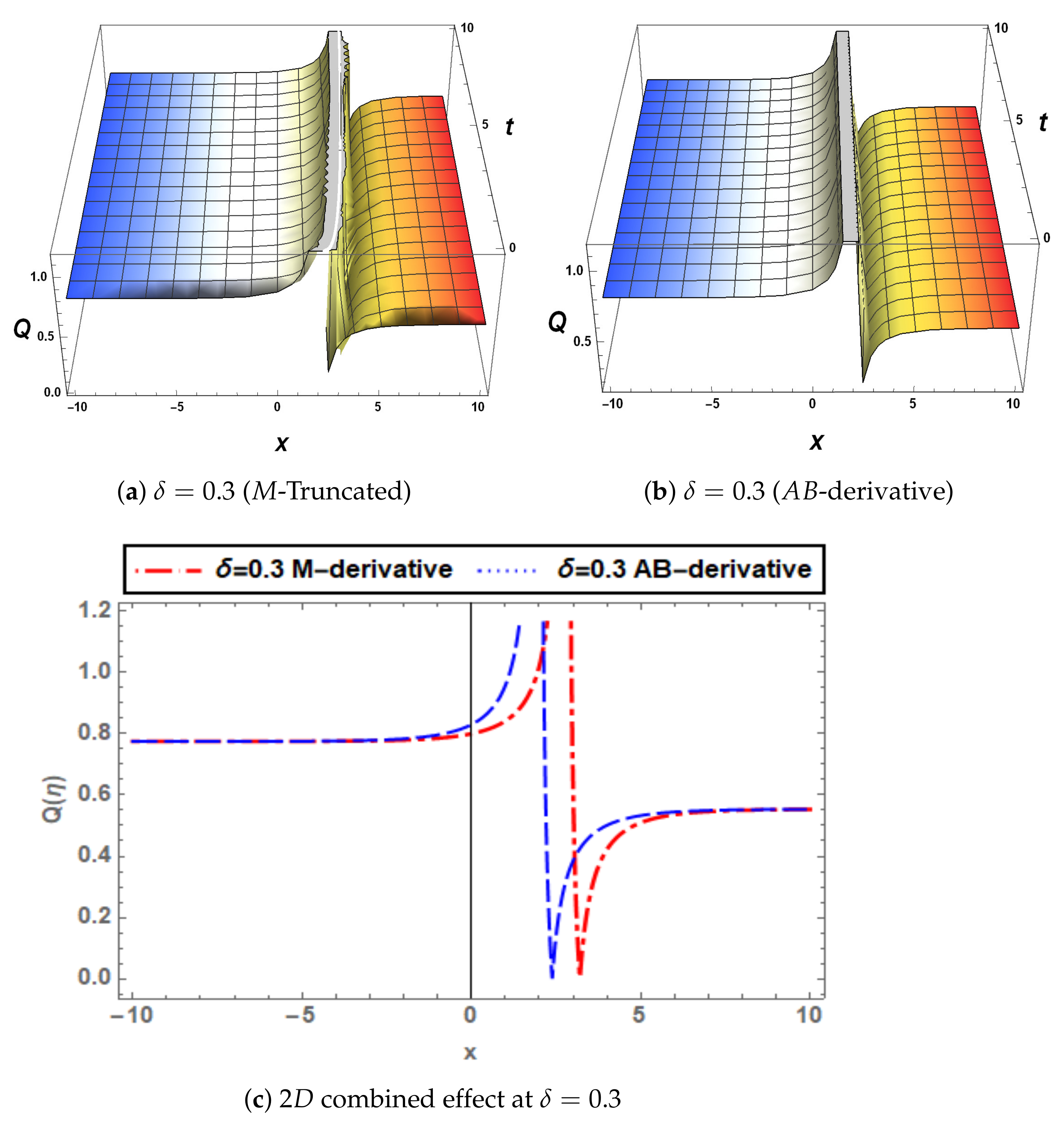
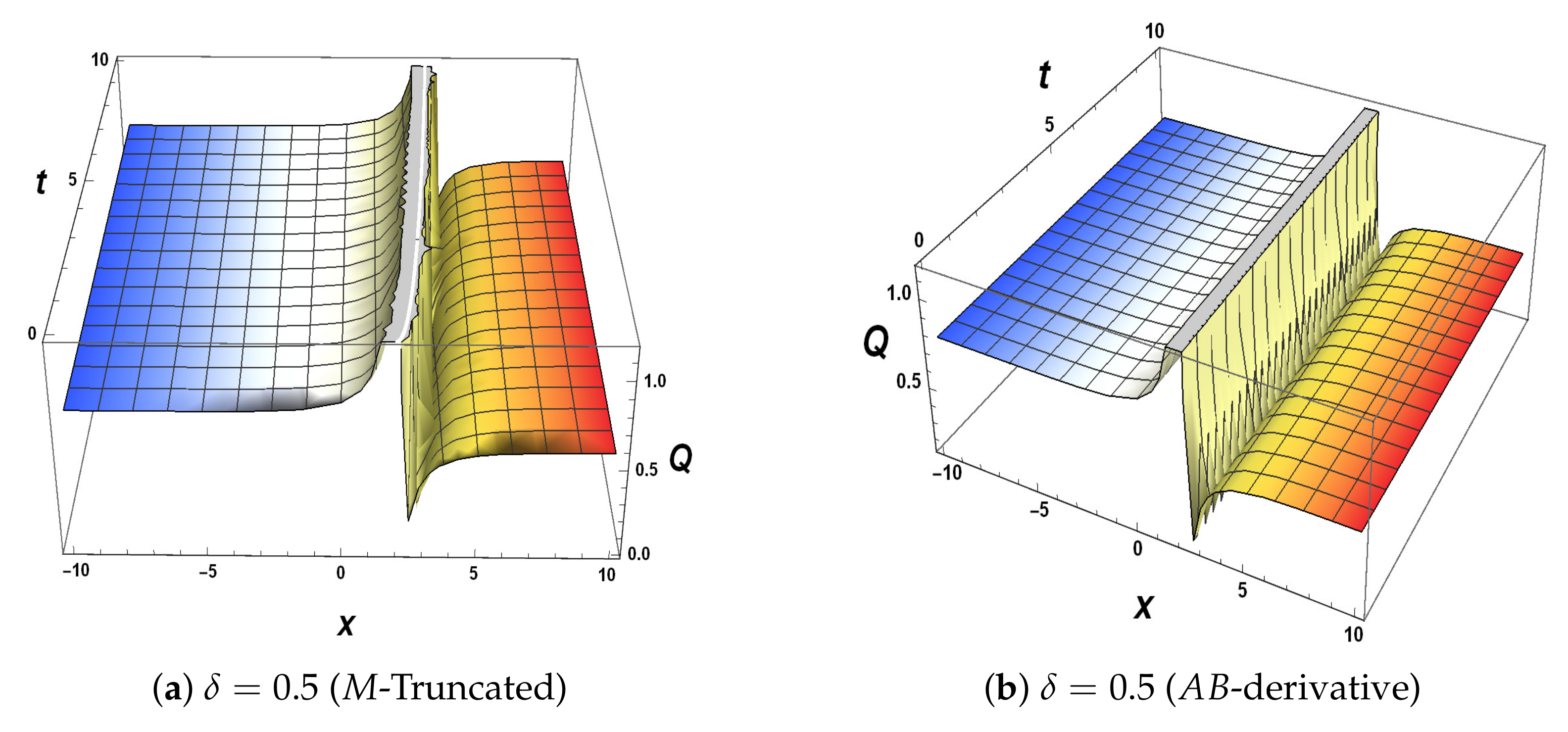
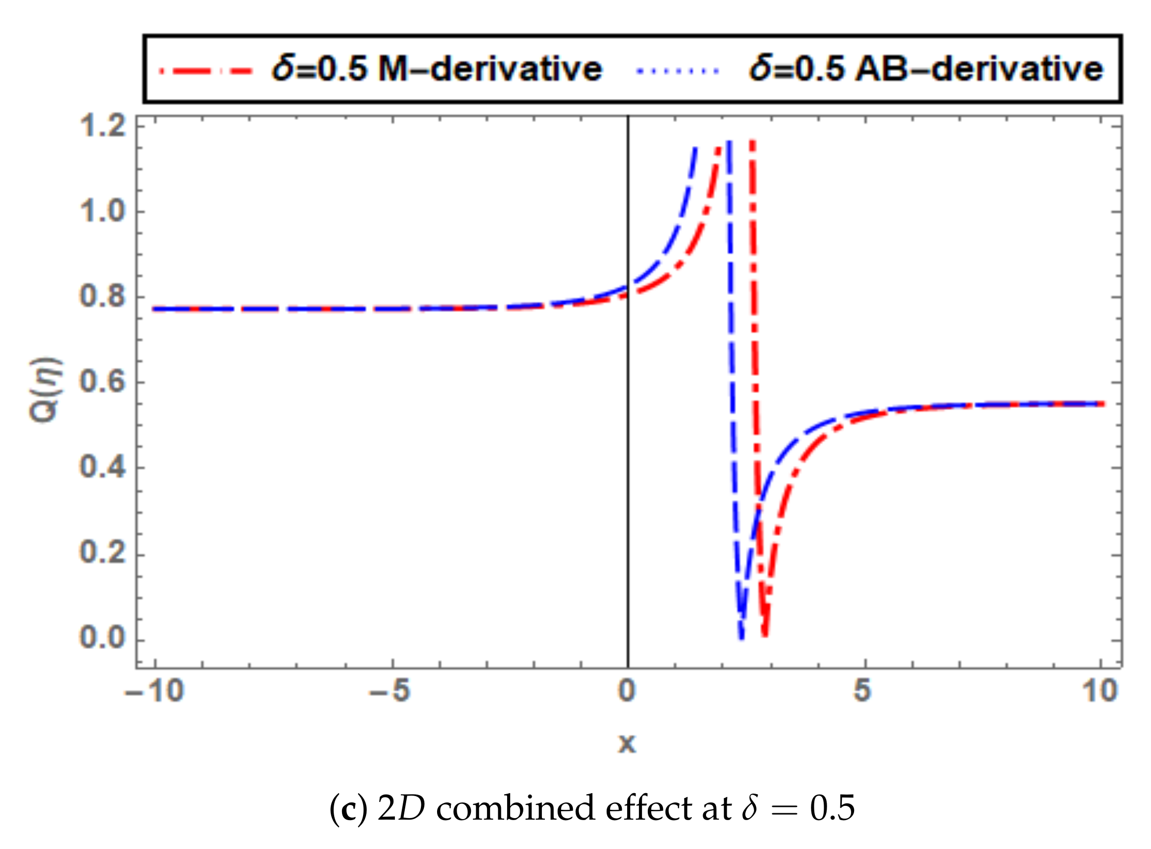
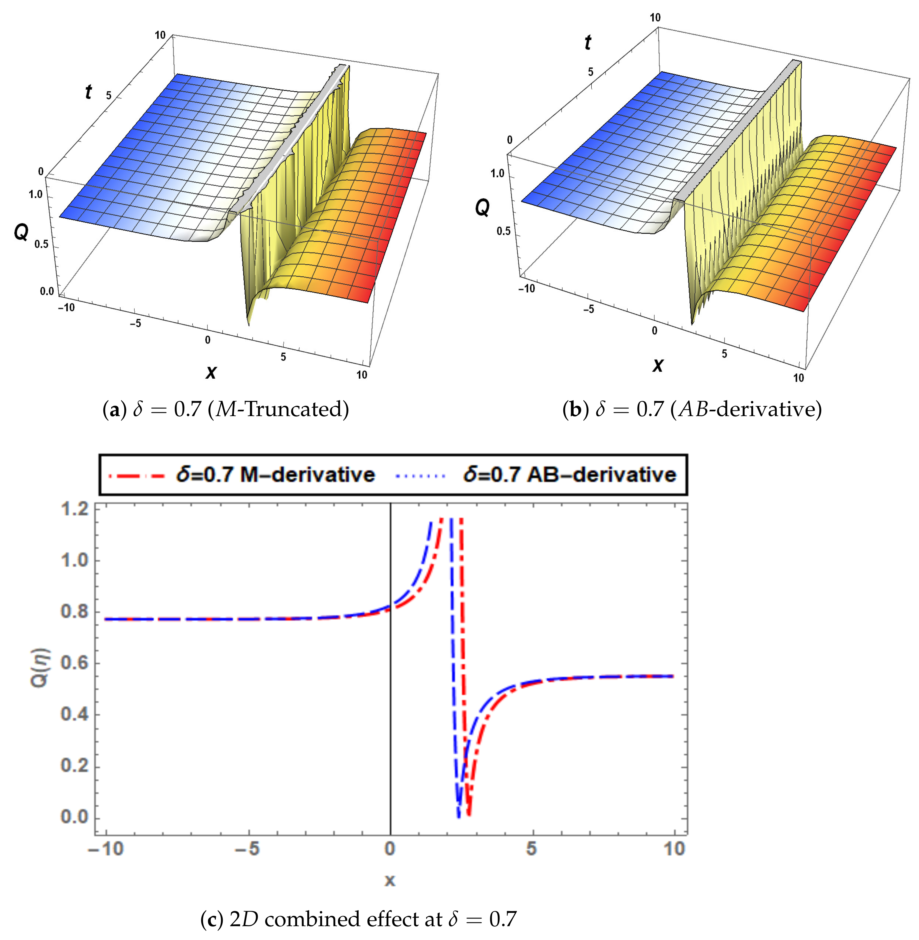
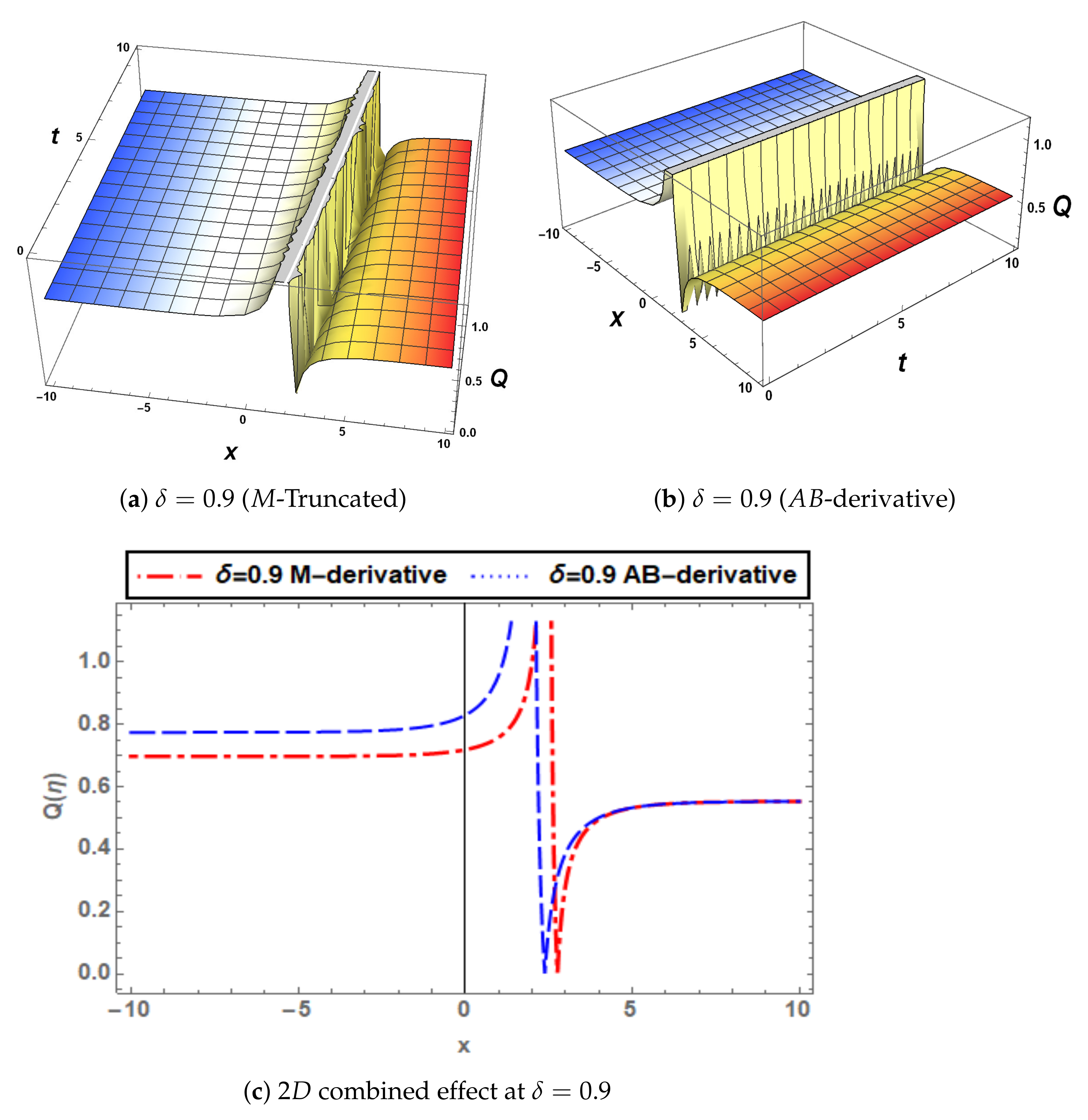
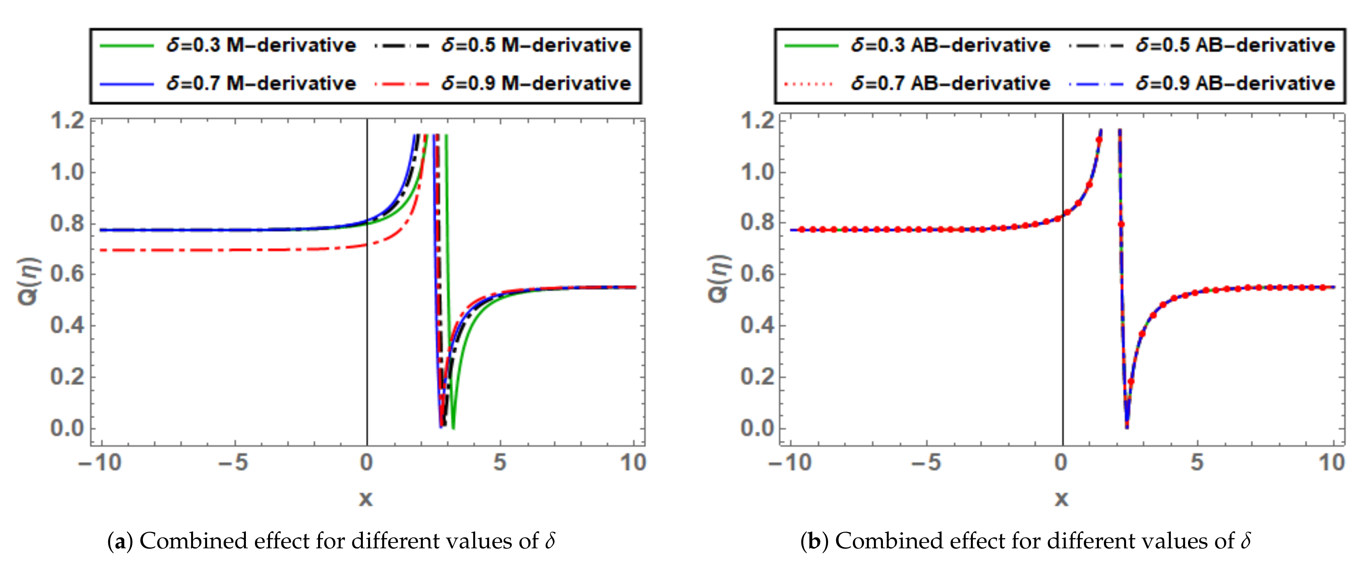
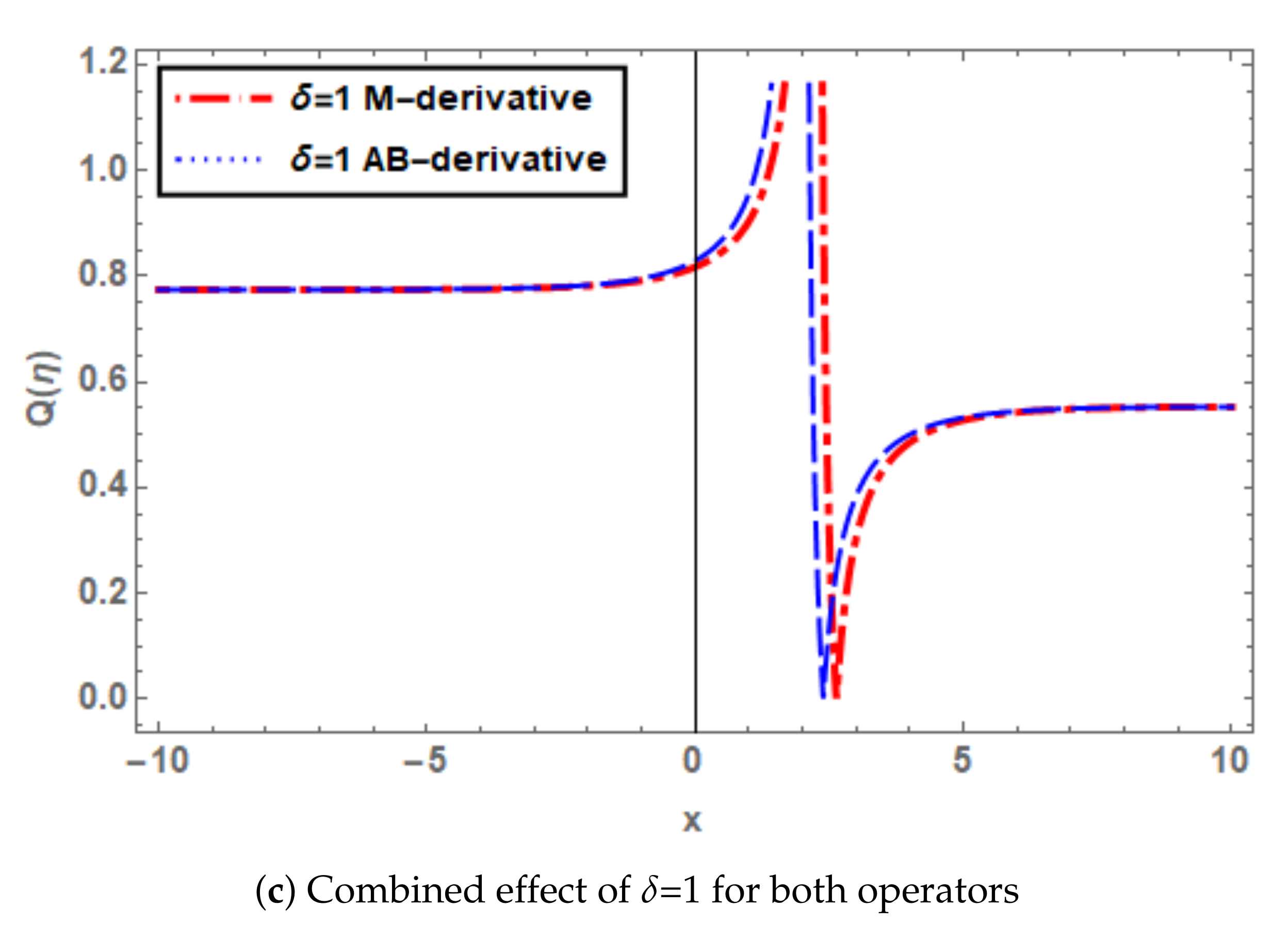
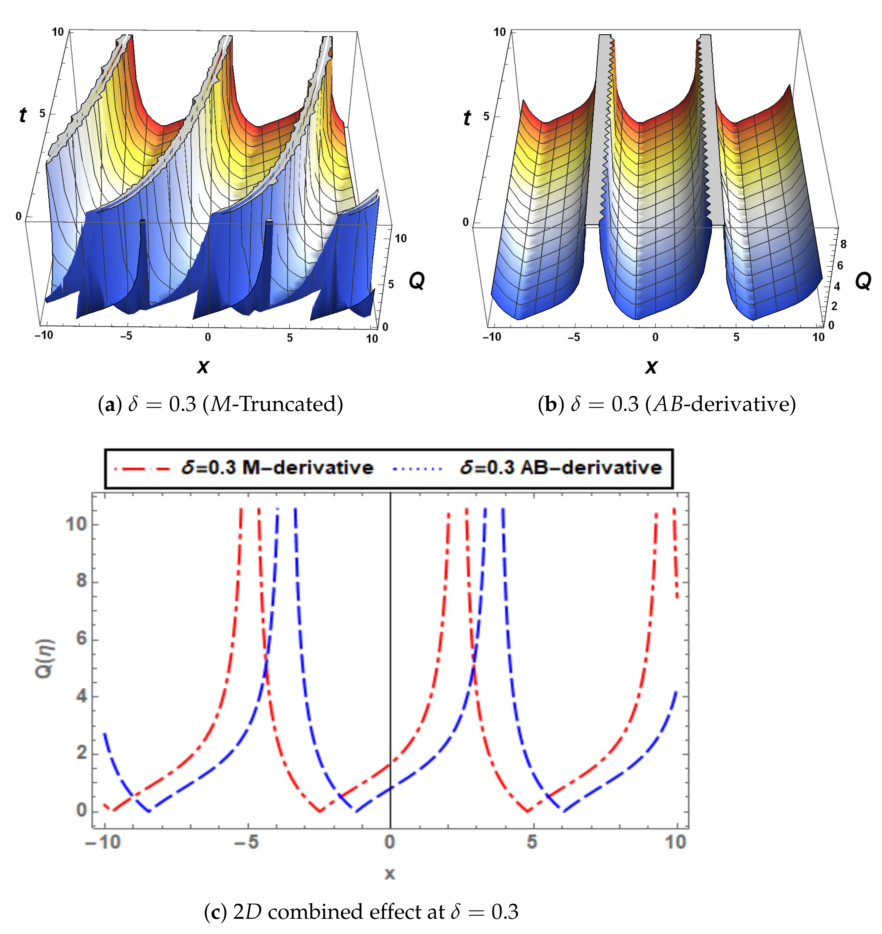
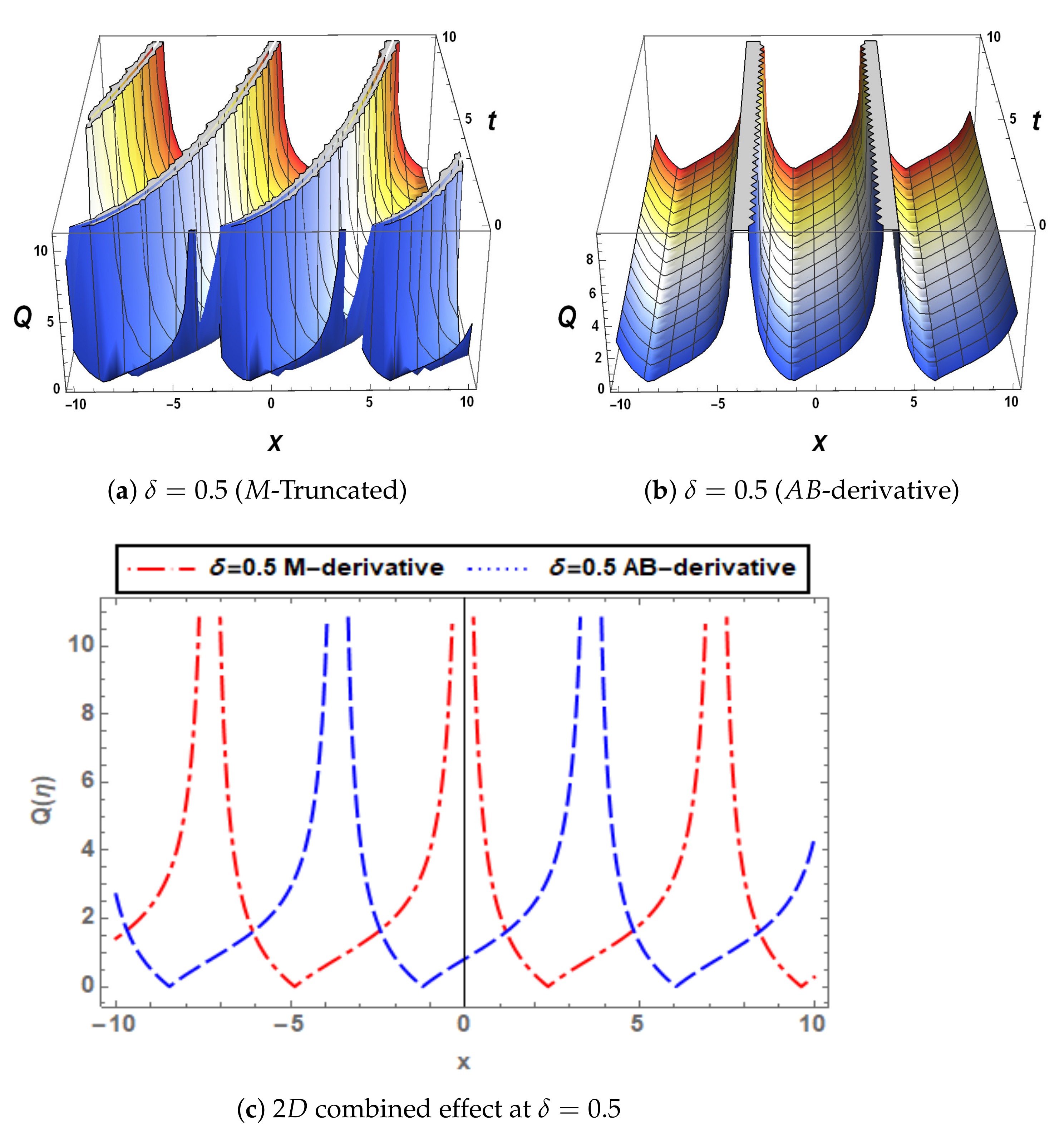
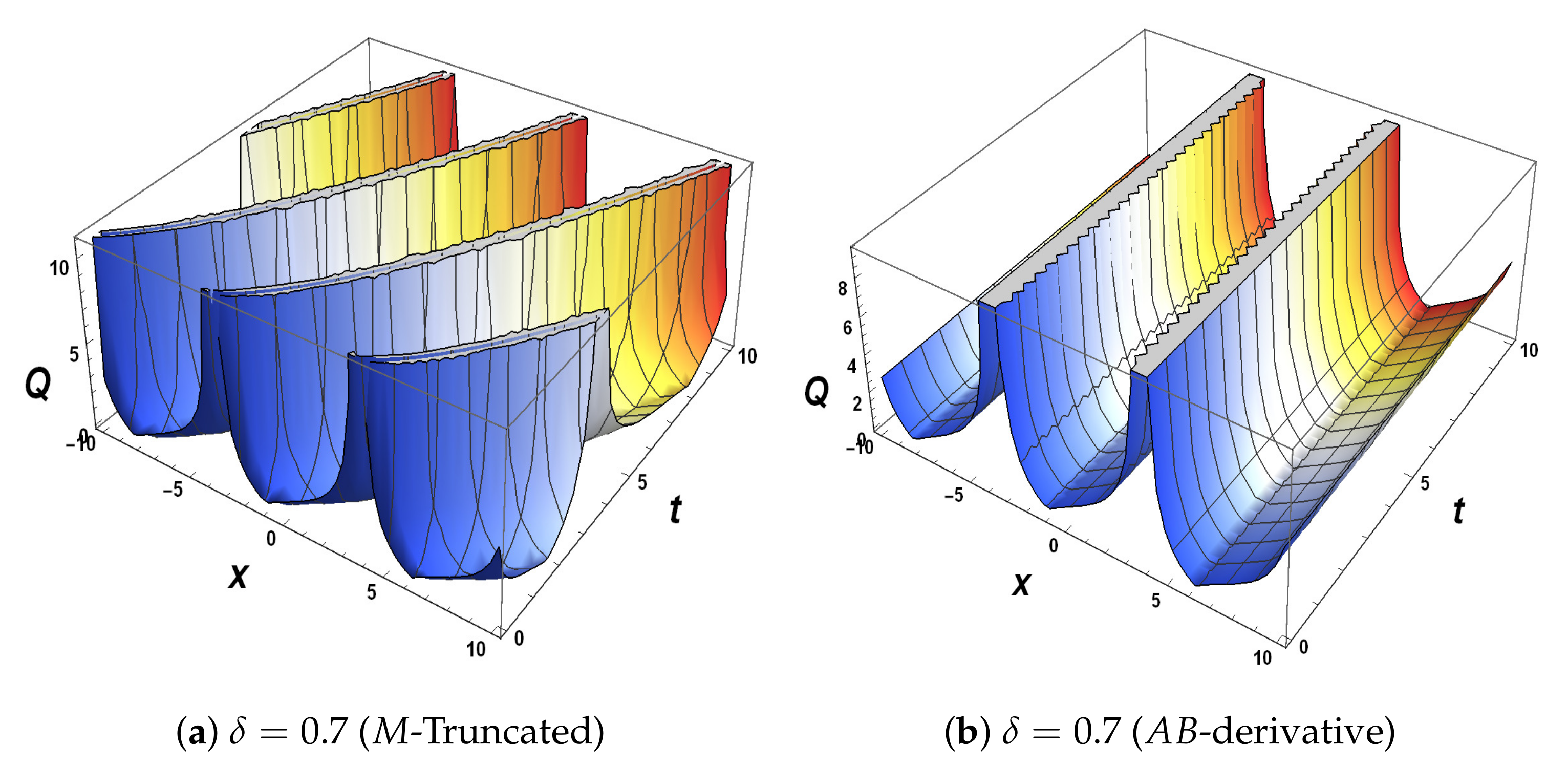
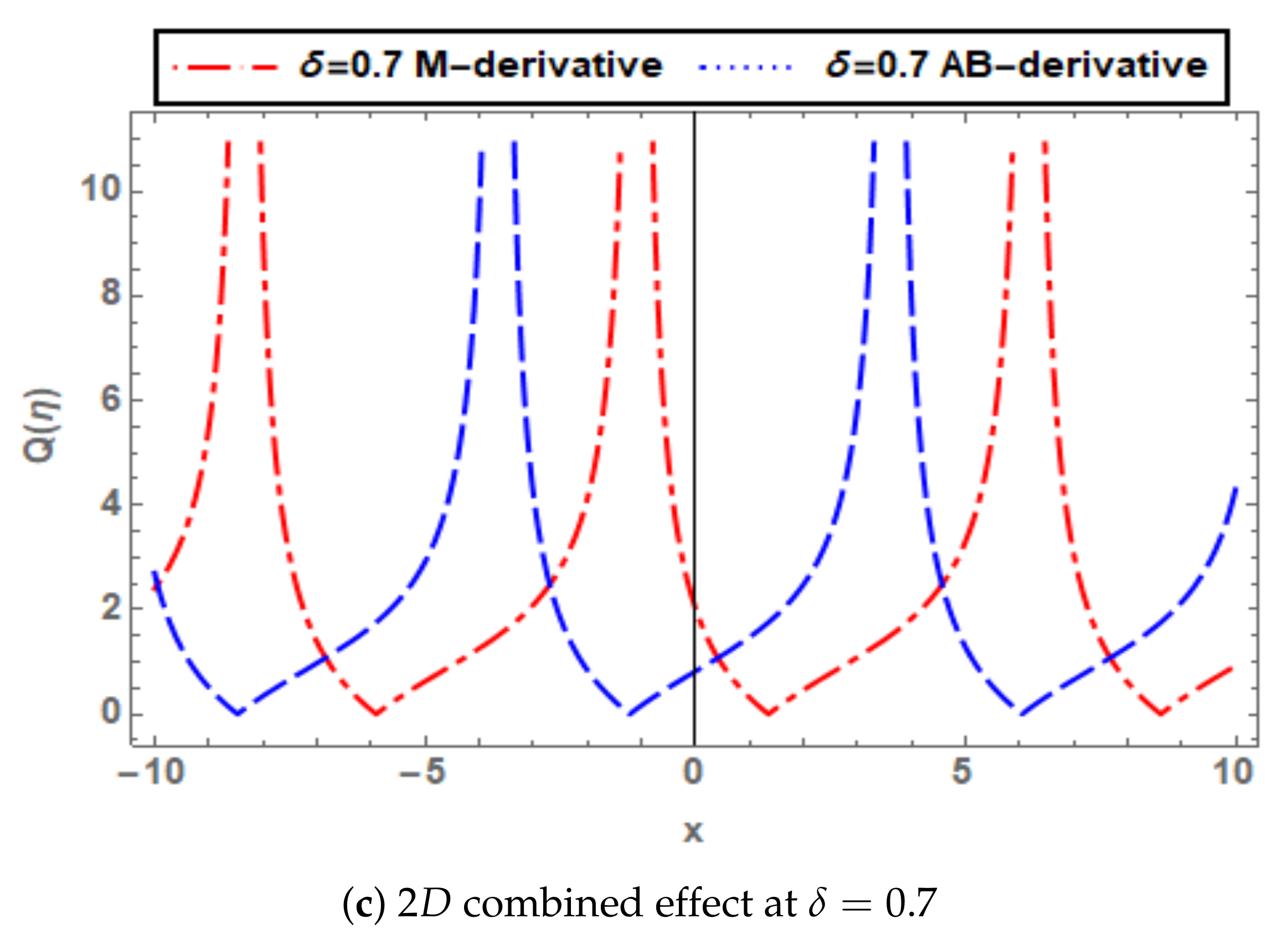
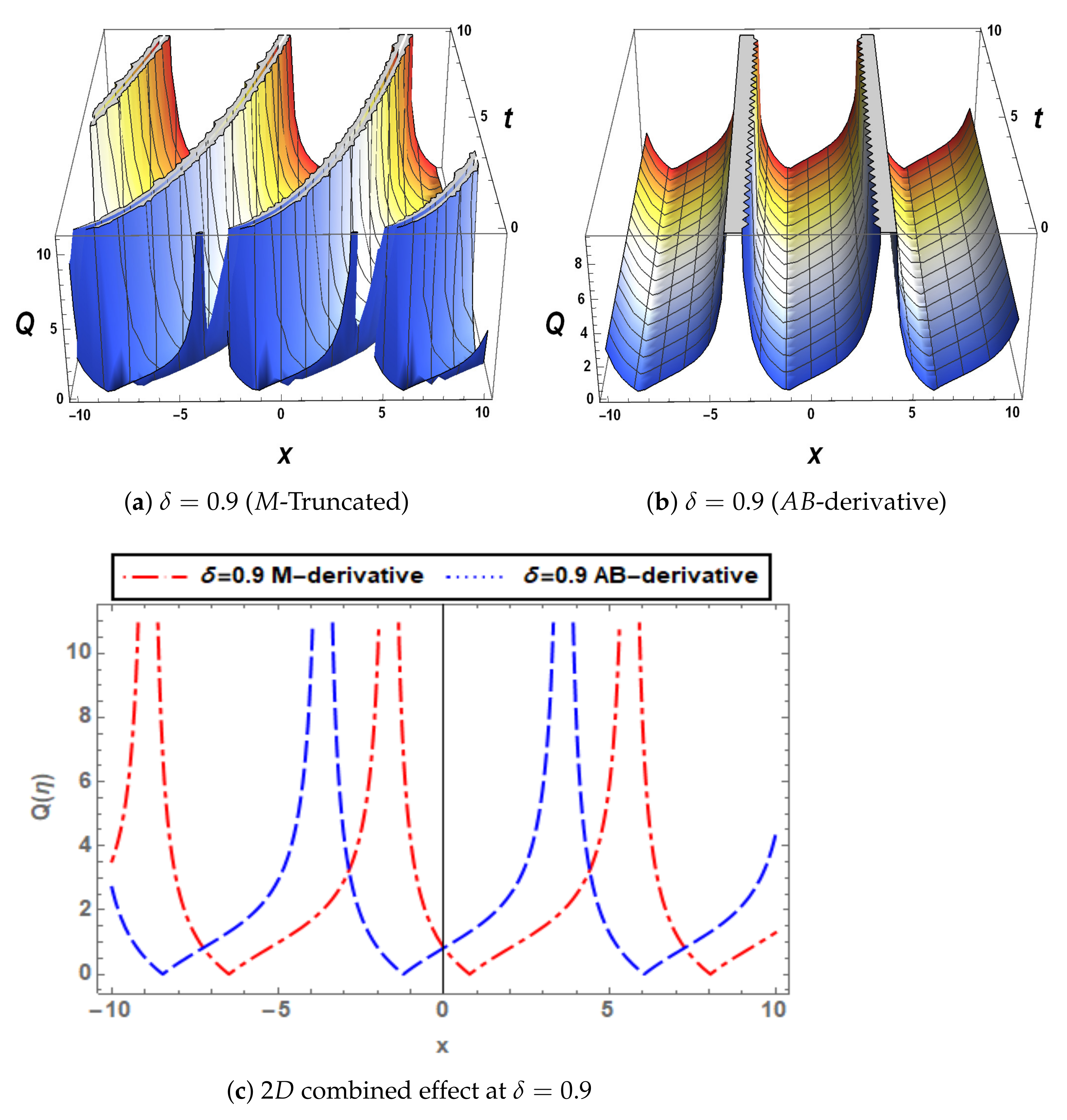
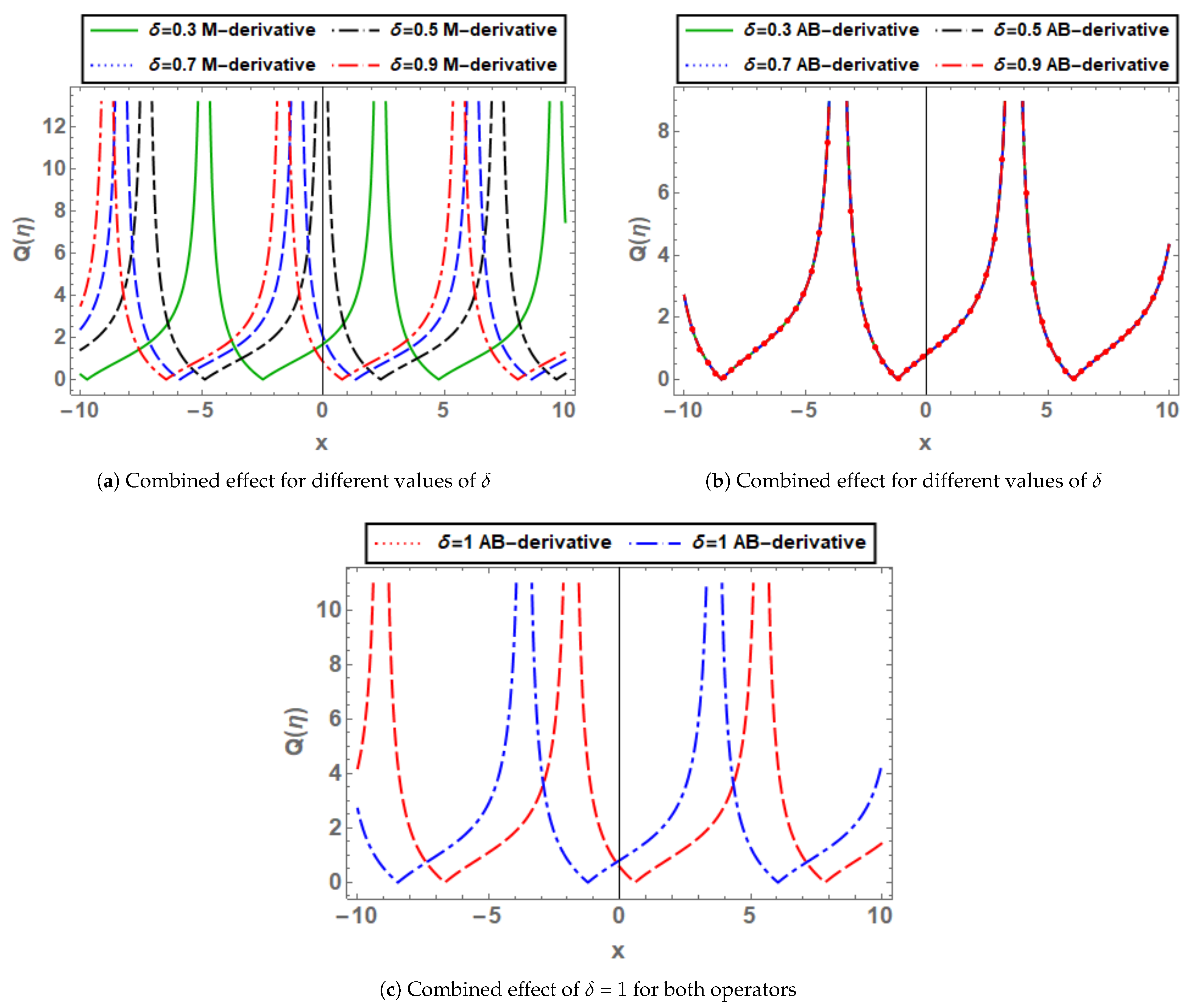
In this part, some of the analytical results of this research are represented graphically. The section mostly focuses on the background understanding of the specific findings investigated in this study. Using a current piece of professional tools of programming, graphs are constructed for clearer illustration. Additionally, each $2D$ and $3D$ graph is shown over a unique time frame. We utilize different colors to ensure that the wave’s behavior will change, that distinct waves will overlap, or that different curves will appear at different points inside the same wave. Depending on the physical regions of the parameters, relevant quantities can be employed. As a key element of our inquiry, we can use changeable characteristic values to examine the distinctive dynamic features, shapes, and patterns of soliton solutions. However, it is important to keep in mind that the solutions also comprise dark functions, bright modules, and trigonometric functions. Here, the fractional MEW equation for M-truncated and $AB$ fractional operators is investigated by NAEM. To analyze the efficacy of operators, we examine the solutions utilizing fractional data points. Figure 1, Figure 2, Figure 3, Figure 4, Figure 5, Figure 6, Figure 7, Figure 8, Figure 9 and Figure 10 depict the graphical representation of two solutions ${\mathcal{Q}}_{14}(x,t)$ and ${\mathcal{Q}}_{16}(x,t)$ and explain the effects of fractional parameter $\delta$ on different values.

Figure 1, Figure 2, Figure 3, Figure 4 and Figure 5:

One such graph represents a physical meaning of ${\mathcal{Q}}_{14}(x,t)$. Plots show the results of applying fractional operators to the given solution while using various non-integer parametric values. Here is a graphical depiction of the acquired result using the parametric values, $\chi =-1$, $\beta =0.7$, $\gamma =0.3$, $\rho =-2$, $\nu =1$, $\theta =\lambda =1$ and $\varrho =0.4$. (a,b) depict $3D$ profiles using M-Truncated and $AB$-fractional operators employing $\delta =0.3$, $\delta =0.5$, $\delta =0.7$ and $\delta =0.9$ at $t=1$.

Figure 6, Figure 7, Figure 8, Figure 9 and Figure 10:

Every such graph betrays a physical meaning of ${\mathcal{Q}}_{16}(x,t)$. Plots display the outcomes of applying multiple non-integer parametric values to the provided solution while utilizing fractional operators. Here is a graphical exhibition of the obtained result using the parametric values, $\chi =2$, $\beta =0.5$, $\gamma =1$, $\rho =-1$, $\nu =2$, $\theta =1.5$, $\lambda =2$ and $\varrho =0.3$. Figures (a,b) depict $3D$ plots using M-Truncated and $AB$-fractional operators assigning $\delta =0.3$, $\delta =0.5$, $\delta =0.7$ and $\delta =0.9$ at $t=1$.

7. Sensitivity Behavior of Fractional MEW Equation

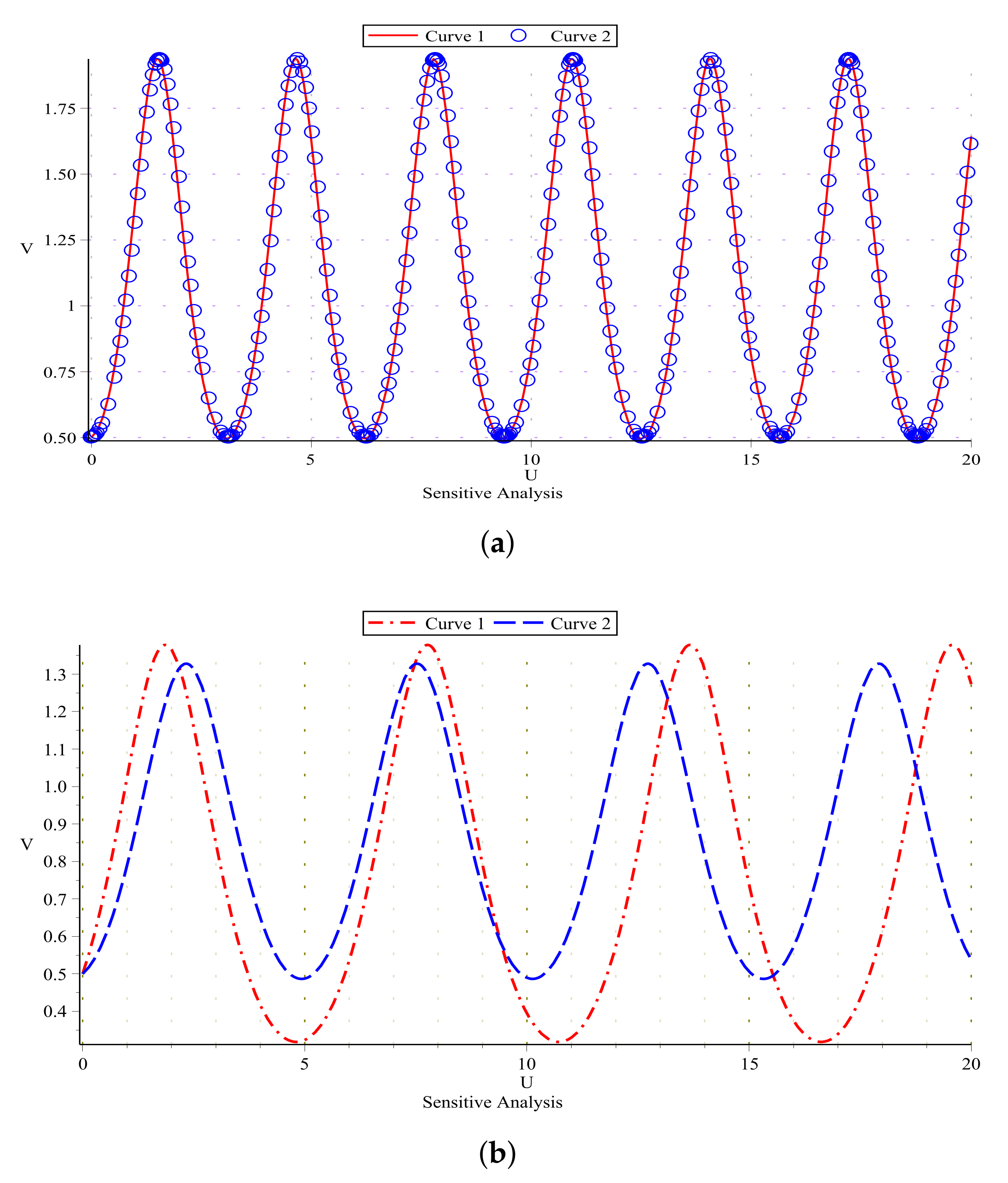
This section discusses the recommended model’s sensitive behavior after it has been converted into a system. Sensitivity is the determination of our system’s sensitivity. A system is lowly sensitive if a slight change in the initial conditions leads to a minor change in the system. As a result, the system is highly sensitive if it changes significantly as a result of a small change in the initial conditions. Accurately assessing the output disruption brought on by input changes is the primary goal of the current investigation. The analysis findings may be shown, which are displayed using a range of parametric values to demonstrate how little changes in input can result in big variances in the outcome. The following is a thorough analysis of the specified system (see Figure 11).

8. Conclusions

In this research, soliton solutions of the fractional MEW equation have been explored using M-truncated and $AB$-derivatives. Several general soliton solutions to the MEW equation have been discovered using the NAEM in this work. Plotting $3D$ plots and $2D$ line graphs for various solutions have revealed the influence of fractional derivatives on the derived solutions graphically. It is also seen in the examined solutions that the wave solution obtains a stable shape substantially faster for the fractional derivatives. The pattern of the obtained wave becomes stable when the value of the fractional order of the derivative approaches unity for the fractional derivative according to a comparison of graphs employing fractional parameters. Furthermore, the achieved results demonstrate that the proposed scheme for extracting optical solitons of MEW equations using fractional operators is extremely simple, convenient, and effective. Dark, bright, periodic solitons, and other soliton solutions have been achieved. Further research in the disciplines of fractional calculus and NLEEs is expected to benefit from the results presented here.

References

- Baleanu, D.; Samaneh, S.S.; Amin, J.; Ozlem, D.; Jihad, H.A. The fractional dynamics of a linear triatomic molecule. Rom. Rep. Phys. 2021, 73, 105. [Google Scholar]
- Ghanbari, D.; Baleanu, D. New optical solutions of the fractional Gerdjikov-Ivanov equation with conformable derivative. Front. Phys. 2020, 8, 167. [Google Scholar] [CrossRef]
- Abouelregal, A.E.; Nofal, T.A.; Alsharari, F. A thermodynamic two-temperature model with distinct fractional derivative operators for an infinite body with a cylindrical cavity and varying properties. J. Ocean. Eng. Sci. 2022. [Google Scholar] [CrossRef]
- Zang, S.; Zong, Q.; Liu, D.; Gao, W. A generalized exp-function method for fractional Riccati differential equations. Commun. Fract. Calc. 2010, 1, 48–51. [Google Scholar]
- Chen, Q.; Baskonus, H.M.; Gao, W.; Ilhan, E. Soliton theory and modulation instability analysis: The Ivancevic option pricing model in economy. Alex. Eng. J. 2022, 61, 7843–7851. [Google Scholar] [CrossRef]
- Atangana, A.; Baleanu, D.; Alsaedi, A. Analysis of time fractional Hunter-Saxton equation: A model of neumatic liquid crystal. Open Phys. 2016, 14, 145. [Google Scholar] [CrossRef]
- Jhangeer, A.; Almusawa, H.; Rahman, R.U. Fractional derivative-based performance analysis to Caudrey-Dodd-Gibbon-Sawada-Kotera equation. Results Phys. 2022, 36, 105356. [Google Scholar] [CrossRef]
- Atangana, A.; Alqahtani, R.T. Modelling the Spread of River Blindness Disease via the Caputo Fractional Derivative and the Beta-derivative. Entropy 2016, 18, 40. [Google Scholar] [CrossRef]
- Akram, U.; Seadawy, A.R.; Rizvi, S.T.R.; Younis, M.; Althobaiti, S.; Sayed, S. Traveling wave solutions for the fractional Wazwaz-Benjamin-Bona-Mahony model in arising shallow water waves. Results Phys. 2021, 20, 103725. [Google Scholar] [CrossRef]
- Veeresha, P.; Ilhan, E.; Baskonus, H.M. Fractional approach for analysis of the model describing wind-influenced projectile motion. Phys. Scr. 2021, 96, 075209. [Google Scholar] [CrossRef]
- Ilhan, E.; Veeresha, P.; Baskonus, H.M. Fractional approach for a mathematical model of atmospheric dynamics of CO2 gas with an efficient method. Chaos Solitons Fractals 2021, 152, 111347. [Google Scholar] [CrossRef]
- Rezazadeh, H.; Osman, M.S.; Eslami, M.; Mirzazadeh, M.; Zhou, Q.; Badri, S.A.; Korkmaz, A. Hyperbolic rational solutions to a variety of conformable fractional Boussinesqlike equations. Nonlinear Eng. 2019, 8, 224–230. [Google Scholar] [CrossRef]
- Sulaiman, T.A.; Bulut, H. Boussinesq equations: M-fractional solitary wave solutions and convergence analysis. J. Ocean. Sci. 2019, 4, 1–6. [Google Scholar] [CrossRef]
- Hu, M.; Jia, Z.; Chen, Q.; Jia, S. Exact Solutions for Nonlinear Wave Equations by the Exp-Function Method. Abstr. Appl. Anal. 2014, 2014, 252168. [Google Scholar] [CrossRef]
- Abdeljabbar, A.; Roshid, H.O.; Aldurayhim, A. Bright, Dark, and Rogue Wave Soliton Solutions of the Quadratic Nonlinear Klein-Gordon Equation. Symmetry 2022, 14, 1223. [Google Scholar] [CrossRef]
- Raza, N.; Rahman, R.U.; Seadawy, A.; Jhangeer, A. Computational and bright soliton solutions and sensitivity behavior of Camassa-Holm and nonlinear Schrödinger dynamical equation. Int. J. Mod. Phys. B 2021, 35, 2150157. [Google Scholar] [CrossRef]
- Jaradat, I.; Alquran, M. A variety of physical structures to the generalized equal-width equation derived from Wazwaz-Benjamin-Bona-Mahony model. J. Ocean. Eng. Sci. 2021, 7, 244–247. [Google Scholar] [CrossRef]
- Abouelregal, A.E.; Alanazi, R. Fractional Moore-Gibson-Thompson heat transfer model with two-temperature and non-singular kernels for 3D thermoelastic solid. J. Ocean. Eng. Sci. 2022. [Google Scholar] [CrossRef]
- Nikitin, A.G.; Barannyk, T.A. Solitary wave and other solutions for nonlinear heat equations. Cent. Eur. J. Math. 2004, 2, 440–458. [Google Scholar] [CrossRef]
- Nguyen, A.T.; Nikan, O.; Avazzadeh, Z. Traveling wave solutions of the nonlinear Gilson-Pickering equation in crystal lattice theory. J. Ocean Eng. Sci. 2022. [Google Scholar] [CrossRef]
- Jhangeer, A.; Muddassar, M.; Rehman, Z.U.; Awrejcewicz, J.; Riaz, M.B. Multistability and dynamic behavior of non-linear wave solutions for analytical kink periodic and quasi-periodic wave structures in plasma physics. Results Phys. 2021, 29, 104735. [Google Scholar] [CrossRef]
- Karpov, P.; Brazovskii, S. Pattern Formation and Aggregation in Ensembles of Solitons in Quasi One-Dimensional Electronic Systems. Symmetry 2022, 14, 972. [Google Scholar] [CrossRef]
- Riaz, M.B.; Baleanu, D.; Jhangeer, A.; Abbas, N. Nonlinear self-adjointness, conserved vectors, and traveling wave structures for the kinetics of phase separation dependent on ternary alloys in iron (Fe-Cr-Y (Y = Mo,Cu)). Results Phys. 2021, 25, 104151. [Google Scholar] [CrossRef]
- Sinha, T.K.; Malla, S.; Baruah, B.; Mathew, J. Long Wave Length Soliton Solutions of Navier Stokes Equation. Int. J. Differ. Equ. 2014, 9, 1–5. [Google Scholar]
- Zayed, E.M.E. A note on the modified simple equation method applied to Sharma-Tasso-Olver equation. Appl. Math. Comput. 2011, 218, 3962–3964. [Google Scholar] [CrossRef]
- Arshed, S.; Raza, N.; Rahman, R.U.; Butt, A.R.; Huang, W.H. Sensitive behavior and optical solitons of complex fractional Ginzburg Landau equation: A comparative paradigm. Results Phys. 2021, 28, 104533. [Google Scholar] [CrossRef]
- Shallal, M.A.; Ali, K.K.; Raslan, K.R.; Rezazadeh, H.; Bekir, A. Exact solutions of the conformable fractional EW and MEW equations by a new generalized expansion method. J. Ocean. Eng. Sci. 2019, 5, 223–229. [Google Scholar] [CrossRef]
- Yildirim, Y.; Mirzazadeh, M. Optical pulses with Kundu Mukherjee-Naskar model in fiber communication systems. Chin. J. Phys. 2020, 64, 183. [Google Scholar] [CrossRef]
- Arshed, S.; Rahman, R.U.; Raza, N.; Khan, A.K.; Inc, M. A variety of fractional soliton solutions for three important coupled models arising in mathematical physics. Int. J. Mod. Phys. B 2021, 36, 2250002. [Google Scholar] [CrossRef]
- El-Shiekh, R.M.; Gaballah, M. New analytical solitary and periodic wave solutions for generalized variable-coefficients modified KdV equation with external-force term presenting atmospheric blocking in oceans. J. Ocean. Eng. Sci. 2021, 7, 372–376. [Google Scholar] [CrossRef]
- Akbar, Y.; Afsar, H.; Al-Mubaddel, F.S.; Abu-Hamdeh, N.H.; Abusorrah, A.M. On the solitary wave solution of the viscosity capillarity van der Waals p-system along with Painleve analysis. Chaos Solitons Fractals 2021, 153, 111495. [Google Scholar] [CrossRef]
- Raza, N.; Hassan, Z.; Butt, A.R.; Rahman, R.U.; Abdel-Aty, A.H.; Mahmoud, M. New and more dual mode solitary wave solutions for the Kraenkel-Manna-Merle system incorporating fractal effects. Math. Methods Appl. Sci. 2022, 45, 2964–2983. [Google Scholar] [CrossRef]
- Zafar, A.; Raheel, M.; Bekir, A. Exploring the dark and singular soliton solutions of Biswas-Arshed model with full non-linear form. Optik 2020, 204, 164133. [Google Scholar] [CrossRef]
- Wang, D.; Sun, W.; Kong, C.; Zhang, H. New extended rational expansion method and exact solutions of Boussinesq equation and Jimbo-Miwa equations. Appl. Math. Comput. 2007, 189, 878–886. [Google Scholar] [CrossRef]
- Kumar, R.; Verma, R.S. Dynamics of some new solutions to the coupled DSW equations traveling horizontally on the seabed. J. Ocean. Sci. 2022. [Google Scholar] [CrossRef]
- Ling, L.; Zhao, L.C.; Guo, B. Darboux transformation and multi-dark soliton for N-component nonlinear Schrödinger equations. Nonlinearity 2015, 28, 3243. [Google Scholar] [CrossRef]
- Li, L.; Duan, C.; Yu, F. An improved Hirota bilinear method and new application for a nonlocal integrable complex modified Korteweg-de Vries (MKdV) equation. Phys. Lett. A 2019, 383, 1578–1582. [Google Scholar] [CrossRef]
- Cheng, W.; Biao, L.; Chen, Y. Construction of Soliton-Cnoidal Wave Interaction Solution for the (2+1)-Dimensional Breaking Soliton Equation. Commun. Theor. Phys. 2015, 63, 549–553. [Google Scholar] [CrossRef]
- Wakil, S.A.E.; Abulwafa, E.M.; Elhanbaly, A.; Abdou, M.A. The extended homogeneous balance method and its applications for a class of nonlinear evolution equations. Chaos Solitons Fractals 2007, 33, 1512–1522. [Google Scholar] [CrossRef]
- Ghafoor, A.; Haq, S. An efficient numerical scheme for the study of equal width equation. Results Phys. 2018, 9, 1411–1416. [Google Scholar] [CrossRef]
- Wazwa, A.M. The tanh and the sine–cosine methods for a reliable treatment of the modified equal width equation and its variants. Commun. Nonlinear Sci. Numer. 2006, 11, 148–160. [Google Scholar] [CrossRef]
- Dogan, A. Application of Galerkin’s method to equal width wave equation. Appl. Math. Comput. 2005, 160, 65–76. [Google Scholar] [CrossRef]
- Uddin, M. RBF-PS scheme for solving the equal width equation. Appl. Math. Comput. 2013, 222, 619–631. [Google Scholar] [CrossRef]
- Gardner, L.R.; Gardner, G.A. Solitary waves of the equal width wave equation. J. Comput. Phys. 1992, 101, 218–223. [Google Scholar] [CrossRef]
- Raslan, K.R.; Ali, K.K.; Shallal, M.A. The modified extended tanh method with the Riccati equation for solving the space-time fractional EW and MEW equations. Chaos Solitons Fractals 2017, 103, 404. [Google Scholar] [CrossRef]
- Shi, D.; Zhang, Y. Diversity of exact solutions to the conformable space-time fractional MEW equation. Appl. Math. Lett. 2020, 99, 105994. [Google Scholar] [CrossRef]
- Zafar, A.; Raheel, M.; Mirzazadeh, M.; Eslami, M. Different soliton solutions to the modified equal-width wave equation with Beta-time fractional derivative via two different methods. Rev. Mex. Fis. 2022, 68, 1. [Google Scholar] [CrossRef]
- Ali, U.; Ahmad, H.; Baili, J.; Botmart, T.; Aldahlan, M.A. Exact analytical wave solutions for space-time variable-order fractional modified equal width equation. Results Phys. 2022, 33, 105216. [Google Scholar] [CrossRef]
- Akram, G.; Sadaf, M.; Zainab, I. Observations of fractional effects of Beta-derivative and M-truncated derivative for space time fractional Phi-4 equation via two analytical techniques. Chaos Solitonsd Fractals 2022, 154, 111645. [Google Scholar] [CrossRef]
- Raza, N.; Jhangeer, A.; Rahman, R.U.; Butt, A.R.; Chu, Y.M. Sensitive visualization of the fractional Wazwaz-Benjamin-Bona-Mahony equation with fractional derivatives: A comparative analysis. Results Phys. 2021, 25, 104171. [Google Scholar] [CrossRef]
- Salahshour, S.; Ahmadian, A.; Abbasbandy, S.; Baleanu, D. M-fractional derivative under interval uncertainty: Theory, properties and applications. Chaos Solitons Fractals 2018, 117, 84–93. [Google Scholar] [CrossRef]
- Zhu, X.; Cheng, J.; Chen, Z.; Wu, G. New Solitary-Wave Solutions of the Van der Waals Normal Form for Granular Materials via New Auxiliary Equation Method. Mathematics 2022, 10, 2560. [Google Scholar] [CrossRef]
- Rezazadeh, H.; Korkmaz, A.; Eslami, M.; Mirhosseini-Alizamini, S.M. A large family of optical solutions to Kundu-Eckhaus model by a new auxiliary equation method. Opt. Quantum Electron. 2019, 51, 1–2. [Google Scholar] [CrossRef]
- Sousa, J.V.C.; Oliveira, E.C.D. A new truncated M-fractional derivative type unifying some fractional derivative type with classical properties. Int. J. Anal. Appl. 2018, 16, 83–96. [Google Scholar]
Figure 1.
A graphical representation of .
Figure 2.
Figure 3.
Figure 4.
Figure 5.
The graphics of .
Figure 6.
Figure 7.
Figure 8.
A graphical depiction of .
Figure 9.
Figure 10.
Figure 11.
(a) represents the sensitivity analysis of the system by allowing the initial conditions and with , and . It is essential to note that overlapping between curves can be seen. (b) here now taking initial conditions and with and it can be observed that by changing the small input in the initial conditions a large change in the output result is displayed.
Publisher’s Note: MDPI stays neutral with regard to jurisdictional claims in published maps and institutional affiliations. |
© 2022 by the authors. Licensee MDPI, Basel, Switzerland. This article is an open access article distributed under the terms and conditions of the Creative Commons Attribution (CC BY) license (https://creativecommons.org/licenses/by/4.0/).
Share and Cite
MDPI and ACS Style
Riaz, M.B.; Wojciechowski, A.; Oros, G.I.; Rahman, R.U. Soliton Solutions and Sensitive Analysis of Modified Equal-Width Equation Using Fractional Operators. Symmetry 2022, 14, 1731. https://0-doi-org.brum.beds.ac.uk/10.3390/sym14081731
AMA Style
Riaz MB, Wojciechowski A, Oros GI, Rahman RU. Soliton Solutions and Sensitive Analysis of Modified Equal-Width Equation Using Fractional Operators. Symmetry. 2022; 14(8):1731. https://0-doi-org.brum.beds.ac.uk/10.3390/sym14081731
Chicago/Turabian StyleRiaz, Muhammad Bilal, Adam Wojciechowski, Georgia Irina Oros, and Riaz Ur Rahman. 2022. "Soliton Solutions and Sensitive Analysis of Modified Equal-Width Equation Using Fractional Operators" Symmetry 14, no. 8: 1731. https://0-doi-org.brum.beds.ac.uk/10.3390/sym14081731
Note that from the first issue of 2016, this journal uses article numbers instead of page numbers. See further details here.