MODeLING.Vis: A Graphical User Interface Toolbox Developed for Machine Learning and Pattern Recognition of Biomolecular Data

Abstract

Many scientific publications that affect machine learning have set the basis for pattern recognition and symmetry. In this paper, we revisit the concept of “Mind-life continuity” published by the authors, testing the symmetry between cognitive and electrophoretic strata. We opted for machine learning to analyze and understand the total protein profile of neurotypical subjects acquired by capillary electrophoresis. Capillary electrophoresis permits a cost-wise solution but lacks modern proteomic techniques’ discriminative and quantification power. To compensate for this problem, we developed tools for better data visualization and exploration in this work. These tools permitted us to examine better the total protein profile of 92 young adults, from 19 to 25 years old, healthy university students at the University of Lisbon, with no serious, uncontrolled, or chronic diseases affecting the nervous system. As a result, we created a graphical user interface toolbox named MODeLING.Vis, which showed specific expected protein profiles present in saliva in our neurotypical sample. The developed toolbox permitted data exploration and hypothesis testing of the biomolecular data. In conclusion, this analysis offered the data mining of the acquired neuroproteomics data in the molecular weight range from 9.1 to 30 kDa. This molecular weight range, obtained by pattern recognition of our dataset, is characteristic of the small neuroimmune molecules and neuropeptides. Consequently, MODeLING.Vis offers a machine-learning solution for probing into the neurocognitive response.

1. Introduction

The total protein profile acquired by capillary electrophoresis offers a practical and cost-wise solution for obtaining a simple proteome with significant sensibility and specificity [1]. However, this classical technique lacks the discriminative and quantification power of modern proteomic methods, i.e., mass spectrometry (not used in this experiment due to financial matters) or simultaneous immune detection.

Hereafter and to propose salivary protein profiles [2] with a higher sensibility, bioinformatics applications, i.e., toolboxes, offer an integrated software environment for better proteome analysis. They provide access to proteomic data formats, analysis techniques, and specialized visualizations for proteograms [3]. Experion^TM Automated Electrophoresis System, i.e., the system offered straightforwardly by the manufacturer, has been used for multiple clinical applications because of its usefulness in quickly offering a graphical visualization of proteomic bands [4]. It can be used as an out-of-the-box feature for biomarker research. However, it lacks better tools for data visualization and exploration. Contrastingly, high-level computing platforms allow a cost-effective and tailored data analysis.

Various application tools have been developed to enable interactive data mining and visual analytics. Examples include RapidMiner [5] and Tableau [6]. The readiness and the limited coding efforts are significant advantages underlining these software applications. The preference of the present study preference is to directly implement the computing code for a more effective software adaptation to the specific experimental data processing requirements. Different programming languages can be used to this end. For instance, Python has received a remarkably growing interest in ML-related applications. Our choice was to rely on MATLAB, a programming language specifically designed to analyze matrix-based data sets, which is typically applied in the automation and standardization of image analysis routines.

The preference for using MATLAB in the present study is to take advantage of the functions for pattern recognition compiled in the Netlab toolbox [7,8]. This interface is a valuable tool that can aid in the exploration, interpretation, and visualization of data in molecular biology, i.e., proteome, transcriptome, or genome [9]. Ottman and colleagues [10] recently used Experion™ Automated Electrophoresis System, which is an automated platform for protein analysis that incorporates LabChip technology into an integrated system that performs multiple electrophoresis steps in one. In this study [10], Experion™ was used to access RNA quality in combination with MATLAB numerical code for data processing. Those tools, working together, permitted the simulation and construction of proteomic models. Likewise, Hou and colleagues [11] have used Cytoscape™, a data visualization bioinformatics tool combined with MATLAB scripts, for data mining and to analyze interactome networks, i.e., the interaction between proteins. Similarly, to optimize the analysis of the numerous data generated by the Experion™ system, we wrote an algorithm using the programming platform MATLAB for data visualization, exploration, and hypothesis-driven biomarker research. Researchers at SalivaTec Laboratory, have recently proposed bioinformatics solutions [12,13] to address the main problem of this study. Hence, this approach aims (i) to complement the already published results and (ii) to address other specific difficulties, i.e., profiling mental health. The use of total protein profile electropherogram has been scarcely used in the study of mental health due to their limitative discriminative and quantification power. Indeed, only a few investigations propose it, e.g., Sultana and colleagues [14].

Symmetry between Psychological and Total Protein Profiles

Symmetry is still a central concept in natural sciences [15,16]; furthermore, its importance for translational neuroscience is similarly essential. In a conceptual framework, this paper tends to provide a parallel between the “Mind-life continuity” concept published by the authors [17] and symmetry. As published by Hipólito and Martins [17], there are two fundamental models for understanding the phenomenon of natural life, which may be considered theoretically asymmetrical, i.e., the symbolic thinking paradigm and the biological organism model. One of the possible reasons for this hypothesis is that the tools used by these paradigms allow the phenomenological aspects of experience to remain hidden by behavioral tests and neuroimaging. With this paper, we propose a symmetrical correlation between cognitive and electrophoretic profiles, providing a nonreductive type of investigation of mind and life, i.e., of brain and proteins. To assess the symmetry between the previously obtained cognitive data [17,18,19] and the biomolecular data published in this paper, we advanced with a machine learning approach to perform pattern recognition of the extensive and complex electrophoretic data.

2. Materials and Methods

This publication involves a molecular analysis through a data mining solution to better overcome the lack of the discriminative and quantification power offered by a simple molecular biology method, i.e., capillary electrophoresis. The data obtained by capillary electrophoresis is usually expressed in kDa and refers to the molecular weight (MW) of proteins that migrate in the electrophoretic gel. In the International System of Units, kDa (1000 Daltons) is the unified atomic mass unit, and Da is defined as 1/12 of the mass of an unbound neutral atom of carbon-12 in its nuclear and electronic ground state and at rest [20]. The notation MW corresponds to the sum of the atomic weight values of the atoms in a molecule and is used in chemistry to determine stoichiometry (quantitative data) in chemical reactions [21]. In our study, the MW is expressed in terms of kDa.

The protein MW is the sum of all protein amino acid MWs. The calculation for the MW is based on the molecular formula of a compound, i.e., the number of each type of atom is multiplied by its atomic weight and then added to the weights of the other atoms. In our experiment, the electrophoretic data are presented in MW of a protein, which depends on the size of the protein in question. MW is frequently used interchangeably with molecular mass in electrophoresis, though technically, there is a significant definition difference. Molecular mass is a measure of mass, and the MW is a measure of force acting on the molecular mass. This assessment aimed to find specific and characteristic molecular profiles in four previously determined subgroups [17]. Thus, it investigated the molecular strata of the mental health subphenomes formerly identified and comprised a sample of 92 young adults, from 19 to 25 years old, healthy university students at the University of Lisbon, with no serious, uncontrolled, or chronic diseases affecting the nervous system. This study comprises the same methodology that led to the establishment of the Neuro.SalivaPrint [12]. However, it advanced with the methods used to create a graphical user interface (GUI) for data visualization and mining the total protein profile, named MODeLING.Vis.

The molecular data published in this study respect the principles for scientific data management referred to as the FAIR data principles [22], i.e., Findability, Accessibility, Interoperability, and Reusability. Henceforth, (i) the metadata unequivocally includes the identifier of the data it designates and is registered in a searchable resource; (ii) the GUI MATLAB code and MODeLING.Vis protocol is open, accessible, and universally implementable, and the metadata are permanently accessible; (iii) the metadata uses a shared language for knowledge representation and a vocabulary that follows FAIR principles, including qualified references; and (iv) the metadata are described with accurate attributes and released with an accessible data usage license including detailed provenance.

2.1. Data Acquisition (Experion^TM Automated Electrophoresis System (Biorad^®)

Once protein separation was complete, the software subtracted background noise, identified and integrated peaks, and assigned their sizes and concentrations. Experion^TM software displays all three forms of data simultaneously: Virtual gel, Electropherogram, and Results table. SalivaTec has already validated this software for salivary protein profiling [1]. Raw data were thus analyzed with Experion^TM software, which had already been used in several profiling studies [23,24,25].

The data analysis workflow, starting with the raw data, included noise filtering, baseline correction, peak detection, and integration of the peak area from sliced electropherograms. Such functions are commonly used by data processing software, such as MassHunter from Agilent Technologies or XCMS [26]. The width of each electropherogram was defined as 0.02 m/z. On average, ExperionTM detected 1000 peaks in each saliva sample, rounded to a decimal of a kDa. The standard deviation of the relative peak areas of the protein-derived peaks was treated automatically by Experion^TM software algorithms and defined to 0.5 kDa. This allowed the best peak acquisition for our data. All peak areas were divided by the area of the internal standard (relative area) to normalize the signal intensities and to avoid capillary electrophoresis detector sensitivity bias among multiple measurements.

2.2. Data Analysis and Processing (MATLAB Toolbox)

Once the full protein profile was acquired, we used a GUI developed in MATLAB as a data processing and exploration tool. The accurate m/z value for each peak detected within the time domain was calculated with a Gaussian curve-fitting m/z domain peak. The alignment of peaks in multiple measurements was done using an expectation–maximization (EM) algorithm to detect representative peaks and MW range intervals. In summary, Gaussian mixture modeling (GMM) is designed to model the data distribution with a set of Gaussian “bell curves”. The mean and the standard deviation of each Gaussian mixture component express the location and the width of these bell curves. Each “bell curve” weight is an additional GMM parameter set. The fit to the data is done iteratively by (1) tuning the weights based on the mean and the standard deviation values of each Gaussian (Expectation step, initialization can be performed with a K-means algorithm) and (2) relying on the computed weights to update the mean and the standard deviation values (Maximization step); hence, the name of the EM optimization method.

Other techniques and software have been used for the same purpose [27,28] with slight modifications. Other authors have used, for instance, the Douglas–Peucker algorithm [29]. From unit m/z electropherograms, our EM algorithm found corresponding peaks across multiple samples and optimized the numerical parameters of the normalization function, as already proposed by Reijenga and colleagues [30].

2.3. Software

The following pieces of software were used:

(i) Experion Imaging software (Biorad^®, Hercules, CA, USA) for proteomic data acquisition, quantification, and treatment;

(ii) MATLAB^TM for data visualization and data exploration of the protein profiles. A specific GUI was created in MATLAB^TM for that purpose: MODeLING.Vis (https://0-doi-org.brum.beds.ac.uk/10.5281/zenodo.7041477, accessed on 30 November 2022). The NETLAB toolbox for MATLAB was also incorporated in MODeLING.Vis to address pattern recognition tasks [8] and can be consulted at https://www.mathworks.com/matlabcentral/fileexchange/2654-netlab (accessed on 30 November 2022).

3. Results and Discussion

The results and their discussion include and analyze the data acquired in:

(1) MODeLING.Vis;

(2) Neuroinflammatory and neuropeptide panel choice.

The variables analyzed are both quantitative/continuous and qualitative/nominal.

3.1. MODeLING.Vis: Development of A Protein Visualization Tool

Are there categorical differences in the protein profiles matching our mental health strata?

Could an unsupervised learning analysis find corresponding electrophoretic signatures?

Could MODeLING.Vis cluster proteins with a high discriminative power?

MODeLING.Vis is a GUI toolbox created to analyze electrophoretic data. MODeLING.Vis data input/output is based on local storage, nonetheless enhancing the reusability of our electrophoretic data. Respecting the FAIR principles [31], we emphasize improving the ability of machines, in this case, a GUI toolbox, to automatically find and use the electrophoretic data, in addition to supporting its reuse by individuals. Henceforth, with the analysis proposed by this study, we supported data discovery through sound data management and maximized the added value by formal scholarly digital publishing.

Firstly, the full raw electropherogram of the Expected Protein Profiles of the 92 neurotypical young adults was obtained. Then Experion^TM Imaging software exported it to a comma-separated values file, “.csv”. This exported raw profile was treated with the same preliminary strategy as in the pipeline oral proteome study, with the raw data of the 22 control subjects (T-1). The pipeline oral proteome study is a preliminary exploratory study that had already been completed and published [18] and justified the rationale for this work. This biomedical analysis methodology [18] was conducted by SalivaTec laboratory and generated preliminary data with a sample size of 22 control subjects (T-1) and five preliminary subjects (T-1 (before and after the experimental procedure)), for which the total protein profiles were characterized by capillary electrophoresis. These raw data, a preliminary Expected Protein Profile workbook, were published as “EPPStrategyDataExport” (https://0-doi-org.brum.beds.ac.uk/10.5281/zenodo.7054406, accessed on 28 November 2022) and can be consulted at: https://tinyurl.com/EPPStrategyDataExport (accessed on 21 July 2022). This workbook consists of six worksheets demonstrating the preliminary strategy applied to the database—six stages were executed.

The first worksheet (first stage: Total) shows the total raw data of the 12 electrophoretic runs performed for all the samples of neurotypical young adults.

The second worksheet (second stage: Total Reviewed) reviewed the previous one, showing only the MW (shown in kDa) and Concentration (ng/µL) for each sample.

The third worksheet (third stage: Total Rounded) rounded the previous variables into decimals, as we did in the Pipeline Oral Proteome Study, and added the new variable “Order” to help sort the samples.

The fourth worksheet (fourth stage: Total Subgroups Sorted) added the following variables: Subphenome and molecular weight’s Color and Molecular Band. A Subphenome is a variable used to define which subgroup the sample belonged to ES = (i), the top phenome of the Experimental group; CS = (ii) the top phenome of the Control group; EI = (iii) the bottom phenome of the Experimental group; and CI = (iv) the bottom phenome of the Control group. Molecular weight’s Color is a variable showing the respective RGB color corresponding to each group. Molecular Bands is a variable that (i) sorted the rounded MW (shown in kDa) according to a crescent kDa and (ii) showed the respective RGB color correspondent, from which an electrophoretic run was executed.

In the fifth worksheet (fifth stage: Total Clustered), in the first part, the variable MolecularBands was repeated according to the number of electrophoretic runs detected (MolecularBandsRep). Then, in the second part, the variable MolecularBandsRep was colored according to the sample’s subgroup using the algorithm “Excel VLOOKUP Function”. This fifth stage originated the variable MolecularBandsSubgroups.

In the sixth worksheet (sixth stage, named “EPPStrategyDataForMOdeLINGVis”), the preliminary final database is shown, which is a triple-entry table. This worksheet used the previously acquired variables (Sample Number; Molecular Bands Subgroups; Concentration (ng/µL)) to create the final table.

Subsequently, this preliminary final database, the “EPPStrategyDataExport” database, was treated to be imported to MATLAB.

First, the section: “Present in the following subphenomes” was added, which comprised binary variables (present/absent) to identify in which subgroup the Molecular Bands were present. Secondly, the preliminary triple entry table was added to the Molecular Bands Summary for each Subject (ex: D01309).

This final full raw electropherogram was published as “ExportForMOdeLINGVis” (https://0-doi-org.brum.beds.ac.uk/10.5281/zenodo.7054551, accessed on 26 November 2022) and can be consulted at: https://tinyurl.com/ExportForMOdeLINGVis (accessed on 8 August 2022). Lastly, the database was implemented in the MODeLING.Vis toolbox and the variables were imported into arrays. Those arrays indexed a linear matrix of the variables: Molecular Bands Subgroups (kDa) and Concentration (ng/µL) of each sample (subject).

One of the limitations of exploring the data with Experion Imaging software (Biorad^®, Hercules, CA, USA) was its incapacity for generating MW intervals and clustering the subjects according to them. Therefore, we developed a toolbox for unsupervised/supervised machine learning, MODeLING.Vis, and assigned it a https://0-doi-org.brum.beds.ac.uk/10.5281/zenodo.7041477 (accessed on 24 November 2022). The GUI MATLAB code, used in our toolbox, is accessible online (https://www.limmit.org/uploads/2/6/8/4/26841837/modeling.vis.zip (accessed on 8 August 2022)), in the LIMMIT laboratory, Faculty of Medicine, University of Lisbon website, as a free and open-source MATLAB toolbox.

To start the GUI MATLAB code, follow the instructions provided by the video tutorial (https://0-doi-org.brum.beds.ac.uk/10.5281/zenodo.7337428, accessed on 30 November 2022) and use the provided electrophoretic dataset “ExportForMOdeLINGVis”, i.e., protLabled.xls on the video tutorial.

On the MATLAB prompt, write:

>> cd C:\...\code (i.e., where the code is unzipped)

>> addpath(genpath(‘./’))

>> limmitGui

MODeLING.Vis includes three separate phases: (i) Data Visualization, (ii) Data Exploration, and (iii) Data Mining.

The first objective of (i) Data Visualization is to transform the independent continuous variable of MWs into molecular intervals through an algorithm based on the EM scheme to fit a Gaussian mixture model to the data in a maximum likelihood framework. The soundness of this computational method acknowledges various bioinformatics applications, with specific reference under the hypothesis of hidden variables underlying the observed features [32].

The algorithm comprises not only the EM component but a definition of other functions to set concentration (ng/µL) thresholds and the quantity of MW intervals (kernels) of interest.

The number of kernels can be set to the number of isolated local maxima from visual data inspection. MODeLING.Vis permits overlaying the GMM fitting curve with the data distribution. If a local maximum has not been captured by a Gaussian component, then a new kernel can be added to the mixture. The mixture can be so defined within a few trials as part of the interactive data processing capabilities of MODeLING.Vis. It can also be possible to terminate the inclusion of new Gaussians once the data likelihood reaches a saturation point. It is, however, noted that the mixture definition through the visual identification of local maxima has been found very effective in the scope of the present work.

As shown in Figure 1, the number of kernels (Gaussian components) was set to 13 because it was the best algorithm to treat our protein profile and the dispersion in our MW. Furthermore, this application was designed to import from other databases other than human salivary electropherograms and had already been positively tested.

The possibility of defining the number of kernels gives the researcher control over the data exploration of his specific dataset. It does not limit it to the constraints of restricted unsupervised machine learning.

We wanted to find and compare among the four subgroups for our specific data and the number of fixed intervals; thus, we defined it as 13 kernels. This decision provided us with the following significant (p < 0.05) intervals of MW:

(A) [9.1;9.8] kDa;

(B) [9.8;10.3] kDa;

(C) [10.3;13.7] kDa;

(D) [13.7;17.5] kDa;

(E) [17.5;21.1] kDa;

(F) [21.1;24.7] kDa;

(G) [24.7;36] kDa;

(H) [36;42.6] kDa;

(I) [42.6;51.5] kDa;

(J) [51.5;65] kDa,;

(K) [65;77] kDa;

(L) [77;149.7] kDa.

Similarly, these intervals are consistent with the ones discovered by the visual analysis of the capillary gels and quantitative electropherograms. Moreover, these intervals are equally compatible with those found in the preliminary study of the 22 control subjects.

Hence, (a) the major density of protein peak dispersion—[12;18] kDa and [43;66] kDa—was statistically and relevantly subdivided into:

(C) [10.3;13.7] kDa;

(D) [13.7;17.5] kDa;

(E) [17.5;21.1] kDa;

(I) [42.6;51.5] kDa;

(J) [51.5;65] kDa.

Similarly, (b) the minor density of protein peak dispersion—[20;40] kDa and [70;145] kDa—was statistically and relevantly subdivided into:

(F) [21.1;24.7] kDa;

(G) [24.7;36] kDa;

(H) [36;42.6] KDa;

(K) [65;77] kDa;

(L) [77;149.7] kDa.

From this analysis, a new range of density of protein peak dispersion was discovered in the lower molecular range, which offered significant relevance to our specific molecular data dispersion—(c) the lower MW density protein peaks:

(A) [9.1;9.8] kDa;

(B) [9.8;10.3] kDa.

All data visualization and analysis are offered as an easy access tool for the researcher, who may update his proteomic dataset and evaluate how the proposed solution reflects her/his data and hypothesis, as shown in Figure 1.

Subsequently, our GUI provided us with (ii) Data Exploration for hypothesis setting and testing. The toolbox was designed to explore not only one type of dataset but also integrate other datasets acquired for the same sample of subjects. As it is, the researcher can feed multiple clinical and molecular datasets: e.g., clinical evaluations, genomic data, immune detection data, etc.

An additional feature of the toolbox allows for the following:

(a) Integration of multiple omics datasets;

(b) Visual access to explore all the subject information, in particular, and the whole sample, in general.

This approach (a) allows the researcher to conduct better her/his multimolecular approaches in datasets (which tend to be multiple) and (b) addresses a possible solution for the increasingly prominent data characteristics of omics methods.

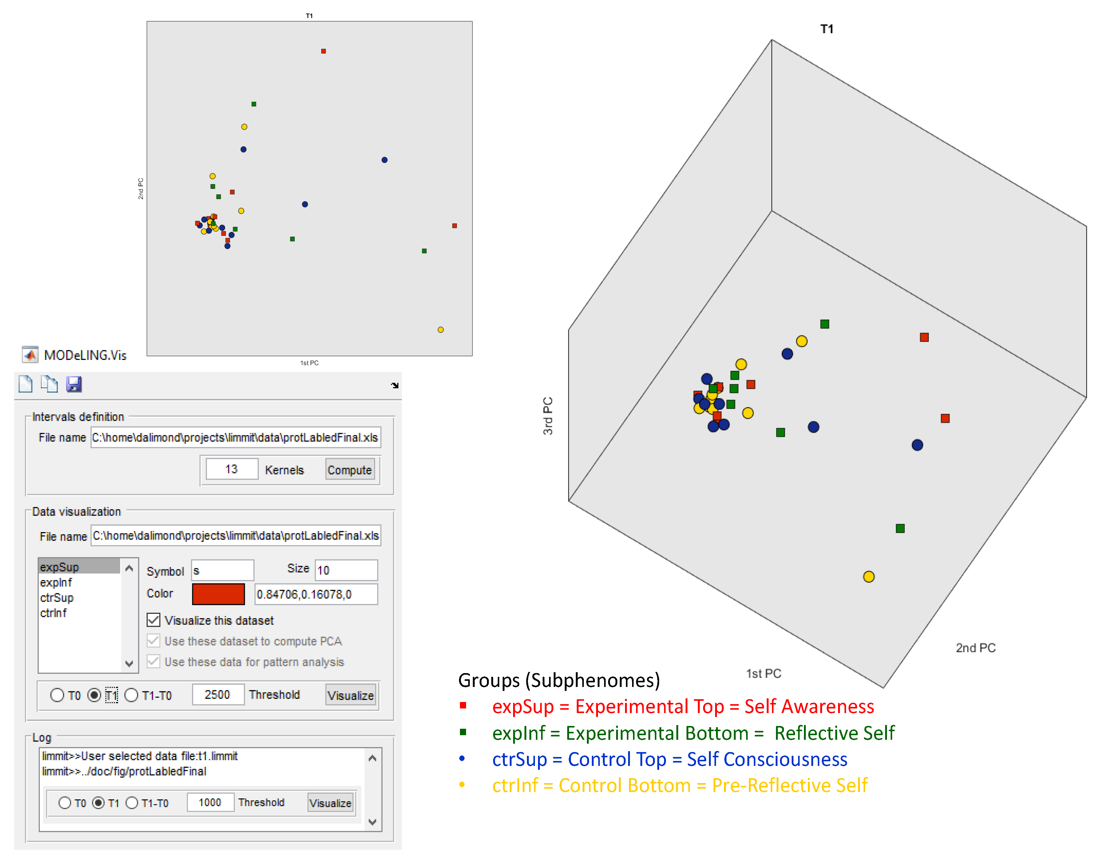
Moreover, as shown in Figure 2, the researcher can define the following:

(a) Colors;

(b) Type of symbol;

(c) Size for the clustering of subgroups.

This configuration eases the identification of specific clusters and makes hypothesis testing more visible. In our study, we created a solution to import T0, T1, and Δ (T1 − T0) datasets and defined the supervised search of the four subgroups. In this part of the data mining, we wanted to feed the algorithm with a specific classification to learn and recognize the four specified labels, which are our subgroups. Moreover, we created the threshold variable for the independent variable (in the case of the electrophoretic data: concentration in ng/µL). The threshold allows the researcher to define how many subjects she or he wants to plot according to the T0, T1, and Δ (T1 x2212; T0) intergroup variability or effect size.

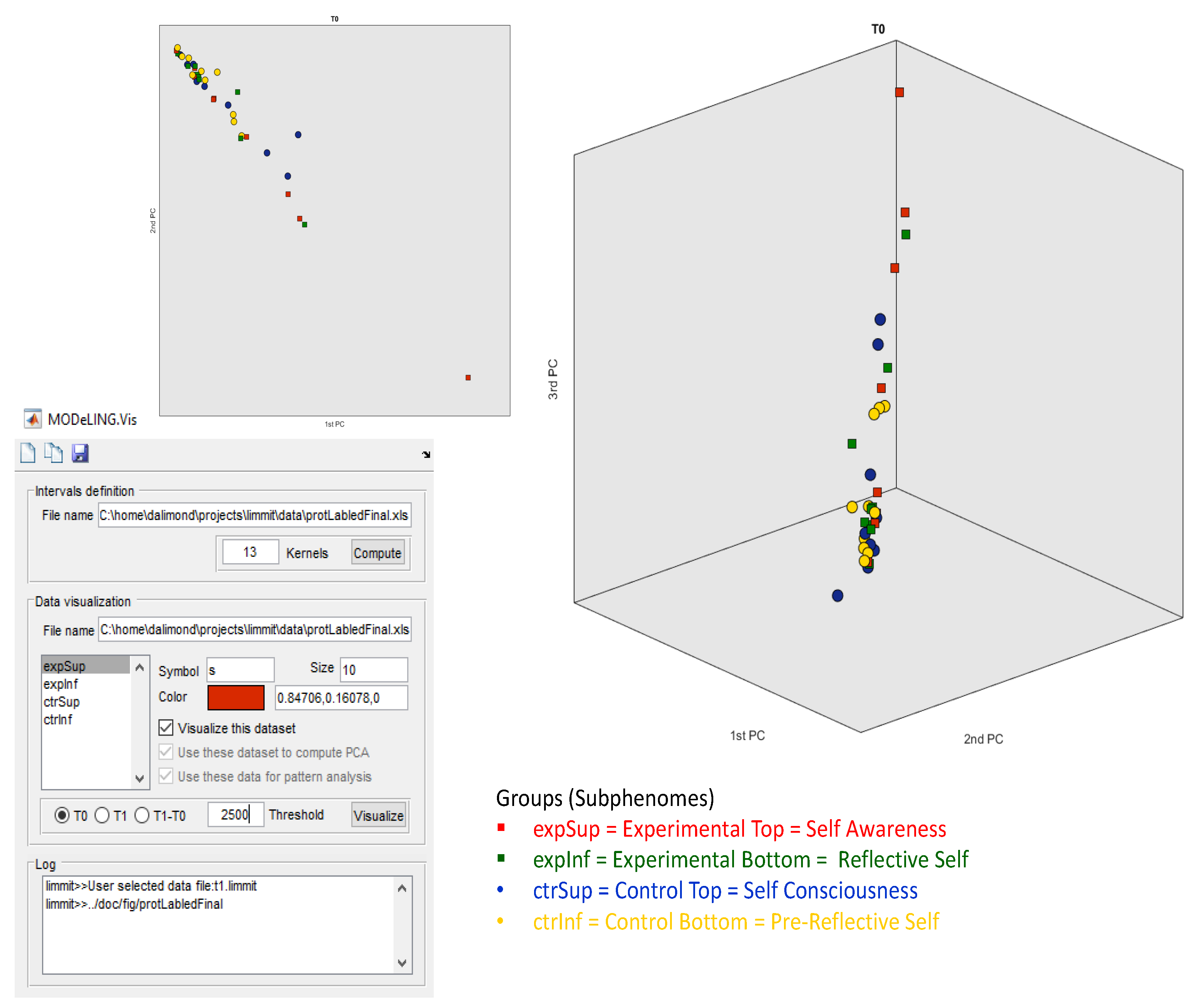
Intergroup statistical testing is performed by simple principal component analysis (PCA), as the data that is routinely fed into the toolbox and its algorithms need an orthogonal linear transformation, which projects the data into a new coordinate system with a reduced number of dimensions, hence allowing for the visualization and interpretation of the data. In Figure 2, the data exploration of our electrophoretic dataset for T0 in MODeLING.Vis is shown. As mentioned, we had the option to define the threshold to 2500 ng/µL because it better fits our data. Then, we set the analysis to T0 and chose the Data Visualization of our electrophoretic data (“ExportForMOdeLINGVis”) and the interval definition acquired before. Finally, we defined colors and symbols for our subgroups. This analysis shows data clusters in only two PCA components and a small, but not very significant, separation of the Experimental Top (red square) and Control Bottom (yellow circle) subgroups.

In Figure 3, the data exploration of our electrophoretic dataset for T1 in MODeLING.Vis is shown. The same parameters were set. This data exploration presents data clustering in three PCA components, and there is a more relevant separation of the Experimental Top (red square) and Control Bottom (yellow circle) subgroups (when compared to T0), which is not visually perceived.

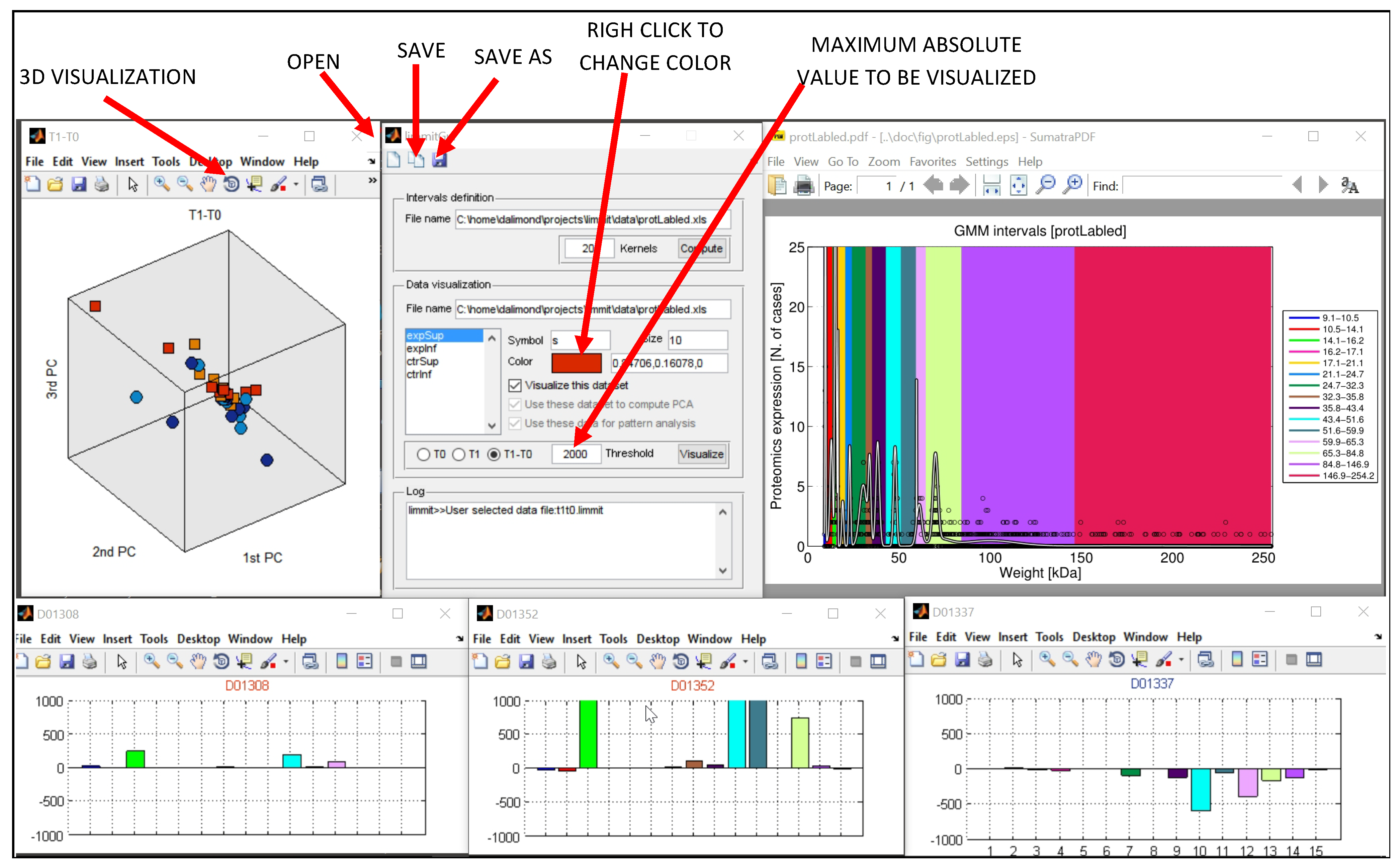
However, this separation is more evident in Figure 4, which shows the data exploration of our electrophoretic dataset for (T1 − T0).

Likewise, the same parameters were set. Nevertheless, in this analysis, data clusters in three PCA components and a significant separation of our cluster of subjects, i.e., clustering in subgroups.

The square symbols (Experimental subgroups), distributed along the top 2PCA and 3PCA axis, are separated from the circle symbols (Control subgroups), spread along the bottom 2PCA and bottom 1PCA axis, with statistical relevance. This approach offers confident consistency for an electrophoretic profile intergroup separation in between the Experimental and Control groups.

Additionally, but not so significantly, there is a separation of the red squares (Experimental Top group) and green squares (Experimental Bottom group), alongside PCA1, and of the blue circles (Control Top group) and yellow circles (Control Bottom group), also alongside PCA1. This offers some consistency for the possibility of an electrophoretic profile separation in between the intra-Experimental electropherograms (Experimental subgroups) and the intra-Control electropherograms (Control subgroups). However, this electrophoretic profile separation is not statistically relevant for a defined threshold Δ (T1 − T0) and effect size of 2500 ng/µL.

More significant is the separation and clustering, both alongside the 3PCA components, between (i) the red squares (Experimental Top group) vs. the blue circles (Control Top group) and (ii) the green squares (Experimental Bottom subgroup) vs. the yellow circles (Control Bottom subgroup).

This data exploration offers some consistency for a possible electrophoretic profile separation between (i) the Experimental Top and Control Subphenomes and (ii) the Experimental Bottom and Control Subphenomes.

This clustering lacks proper hypothesis testing to evaluate the exact concentration (ng/µL) of the Δ (T1 − T0), which is the main limitation of this analysis.

Notwithstanding, it may offer the opportunity to define a consequent hypothesis, i.e., to better profile and stratify substrata in our total electrophoretic data. Therefore, the subsequent data analysis was executed as a reasonable solution for this limitation.

The toolbox has the objective of (iii) Data Mining the individual molecular profile (subject to subject/sample to sample) and comparing it to the whole sample (neurotypical young adults).

As referred, it was designed to integrate multiple clinical and molecular datasets.

As such, in Figure 4, we present an example of the comparison of four subjects after the phases of the GUI toolbox:

(i) Data Visualization;

(ii) Data Exploration;

(iii) Data Mining.

We show, fittingly, subject D01383 (Experimental Top subgroup (1)), subject D01371 (Experimental Bottom subgroup (3)), subject D01337 (Control Top subgroup (2)), and subject D01319 (Control Bottom subgroup (4)).

These four subjects (with the same colors) are the most significant subjects of each subgroup and represent the specific and characterizing stratum of the electrophoretic profile of their subgroup.

From the molecular intervals found, those which are more relevant are the red (No. 2) and the pink (No. 4) ones, which correspond to (B) [9.8;10.3] kDa and (D) [13.7;17.5] kDa in the lighter MW range (Figure 1).

Additionally, with a correspondent relevance are the purple (No. 9) and light blue (No. 10) ones, which correspond to (I) [42.6;51.5] kDa and (J) [51.5;65] kDa in the heavier MW range (Figure 1).

The Δ (T1 − T0) ng/µL of the (B) [9.8;10.3] kDa and (D) [13.7;17.5] kDa molecular weight range is for:

(1) Subject D01383 (representing the Experimental Top group) ≅ 50 ng/µL and −900 ng/µL;

(2) Subject D01337 (representing the Control Top group) ≅ −10 ng/µL and −30 ng/µL;

(3) Subject D01371 (representing the Experimental Bottom group) ≅ 600 ng/µL and 800 ng/µL;

(4) Subject D01319 (representing the Control Bottom group) ≅ 0 ng/µL and 2000 ng/µL.

Those MW ranges [(B) [9.8;10.3] kDa and (D) [13.7;17.5] kDa] are characteristic of molecules that have been documented to cross the blood-brain barrier [33] (Banks, 2009). Please note that an error variable should be considered and correspond to the lack of accuracy offered by Experion^TM analysis and the identified MW ranges. This consideration should take this inaccuracy into account, but also the process of protein degradation observed and well documented in saliva.

Different molecular characteristics are associated with the capacity to cross the blood-brain barrier, a significant field of study in neuropharmacology [34,35].

However, in the interest of molecular biology, it is essential to understand those small molecules’ physiology and biological function.

Banks [36] has described the biological characteristics of those small peptides crossing the blood-brain barrier and correlated them to the neuropeptide response. Likewise, this light MW [(B) and (D)] range was earlier associated with neuroinflammatory response [37]. Still, more recently, Erickson and Banks [38] described it as part of the neuroimmune axes of the blood-brain barriers and blood-brain interfaces.

Please note that uncertainties should be considered, which correspond to the lack of accuracy offered by Experion^TM analysis and the identified MW ranges. In addition to this inaccuracy, the process of protein degradation observed and well-documented in saliva should be considered.

Hence, the importance of these small peptides, detected by capillary electrophoresis in this light MW [(B) and (D)] range, for the physiological and pathological regulation of neurotypical/atypical subjects.

The Δ (T1 − T0) ng/µL of the (I) [42.6;51.5] kDa and (J) [51.5;65] kDa molecular weight range is for:

(1) Subject D01383 (representing the Experimental Top group) ≅ −100 ng/µL and 0 ng/µL;

(2) Subject D01337 (representing the Control Top group) ≅ −600 ng/µL and −400 ng/µL;

(3) Subject D01371 (representing the Experimental Bottom group) ≅ 2200 ng/µL and 2000 ng/µL;

(4) Subject D01319 (representing the Control Bottom group) ≅ 900 ng/µL and 800 ng/µL.

Those MWs are characteristic of a group of larger systemic molecules, which have not been documented to cross the blood-brain barrier [33] (Banks, 2009).

Hence, they are not directly relevant to our study as they are not brain-produced proteins but indirectly important as systemic protein expression. In another oriented study design, they could be interesting for heavier protein molecular profiling of the subjects with systemic-produced proteins.

Specifically, this heavier MW range is essential for comprehending the role of larger proteins and protein complexes in non-neuropsychiatric diseases.

As an example, proteins, such as alpha-1-antitrypsin, 47 kDa [39], pyruvate kinase PKM, 58 kDa [40], and serum albumin, 69 kDa [41], are essential markers for hereditary, metabolic, and cardiovascular diseases, respectively.

As a hypothesis for better conduction of our study and better statistical generalization power, it is essential to quantify those lighter MW ranges, i.e., (B) [9.8;10.3] kDa and (D) [13.7;17.5] kDa with more accurate sensibility and sensitivity.

The quantification and identification of those lighter MW ranges are imperative to understand better what is affecting this electrophoretic profile.

However, acquiring data with the ExperionTM automated electrophoresis system (Biorad^®) offers a low capacity to discriminate which proteins reflect that stratum.

This low capacity is explained because electrophoretic patterns refer to a conjunction of proteins that migrate to the same MW and not a specific and single protein migration, and an error correspondent to the lack of accuracy offered by Experion^TM analysis.

A better acquisition method, with higher sensitivity, sensibility, and discrimination, is necessary to explain which proteins are changing.

Identifying those specific proteins can improve our understanding of how they influence the total protein profile in those light molecular ranges: [9.1;30] kDa.

This specific molecular range reflects the whole spectrum of peptides, peptide complexes, and small proteins that migrate in electrophoresis in (c) the lower MW density protein peaks.

For that purpose, simultaneous immune detection, with specific antibodies for specific peptides in those MW ranges, is mandatory for adequate quantification and discrimination.

Moreover, this quantification offers a suitable possibility for multivariate hypothesis testing of the identified peptides and proteins by immune detection.

Following the work of Banks [33,36] and the objective of our study design, immune detection of the peptides and the small proteins implicated in the neuropeptide and the neuroinflammatory response should be addressed.

This identification is essential for better characterization of the protein strata in this light MW range and understanding of how they affect neurotypical young adults.

3.2. Neuroinflammatory and Neuropeptide Panel Choice

A MODeLING.Vis analysis helped us understand which proteins are responsible for the changes observed in the MW range [9.1;30] kDa.

The [9.1;30] kDa MW interval corresponds to small proteins like the ones already identified in saliva by Rosa and colleagues [42] and listed in the OralCard by Arrais and colleagues [43]:

Histatin-1, 7 kDa;

Submaxillary gland androgen-regulated protein 3B, 8 kDa;

Acyl-CoA-binding protein, 10 kDa;

Protein S100-A8, 11 kDa;

Cystatin-A, 11 kDa;

Protein S100-A9, 13 kDa;

Profilin-1, 15 kDa;

Fatty acid-binding protein, 15 kDa;

Cystatin-SA, 16kDa;

Cystatin-SN, 16 kDa;

Cystatin-S, 16 kDa;

Cystatin-C, 16 kDa;

CALML3, 17 kDa;

PIP, 17 kDa;

PRH1, 17 kDa;

Interleukin-1 receptor antagonist protein, 20 kDa;

Glutathione S-transf P, 23 kDa;

HSP β-1, 23 kDa;

ZG16 homol β, 23 kDa;

BPI fold-containing family A member, 27 kDa;

14-3-3 protein sigma, 28 kDa;

Kallikrein-1, 29 kDa.

The listed proteins are small enough either (i) to pass the blood-brain barrier or (ii) to be detected in saliva.

Those proteins have not only well-known neurological functions, for instance, Cystatin-C in amyotrophic lateral sclerosis [44], but may also be altered in neurodevelopmental conditions, for instance, Interleukin-1 receptor antagonist protein (part of the neuroimmune system) in intellectual disability [45].

The best four subjects of the (1) Experimental Top, (2) Control Top, (3) Experimental Bottom, and (4) Control Bottom subgroups are plotted.

These four subjects represent the molecular profile with more significant intergroup variability and intragroup homogeneity.

Therefore, they are the subjects more characteristic of each group and have a more representative molecular profile.

Henceforth, we chose those four subjects of each four subgroups to perform the following analysis. Additionally, we selected one control subject for each group.

As the objective of the following analysis was (i) to study the MW range considered for particles passing the blood-brain barrier and (ii) to probe into the neuroinflammatory and neuropeptide system, we chose one control subject of each subgroup with an inflammatory disease, undergoing the same cognitive load and task.

The subjects followed the analysis already discussed in (ii) the Expected Protein Profile Results.

The Experion^TM Automated Electrophoresis System (Biorad^®) analysis was repeated, but in this case, for those five subjects (4 best + 1 control) of each group. The final objective of this analysis was to evaluate if those five subjects should advance for simultaneous immune detection and quantification.

We want to warn about the limitations of conducting such an analysis and hypothesis testing.

This nonblind analysis lacks the statistical power for generalization for the researcher, and it would be a type 1 statistical error to act as such.

However, such an exploration is valid as an exploratory study aiming at the sole understanding of the protein expression in this small MW range.

Therefore, the most significant protein profiles were selected. This (c) lower MW range [9.1;30] kDa was one of the protein density peaks with more intergroup concentration (ng/µL) difference and intragroup curve similarity.

This [9.1;30] kDa interval is known as characterizing neuroinflammatory response [46], as well as neuropeptide response, as published in the NeuroPep database [47].

The cytokines, interleukins, and neuropeptides are small proteins that migrate in the electrophoresis in this molecular range.

Hence, the vital role that those small neuroimmune molecules [48] and small neuropeptides [49] may have in neurodevelopmental conditions; e.g., autism spectrum disorder [50].

In the following pictures, two molecular ranges should be separated.

From the [9.1;30] kDa range studied, interval I. [9.1;17] kDa, corresponding to the electropherogram’s first peaks, is associated with the smallest molecules of neuropeptide response.

Complementarily, interval II. [17;30] kDa corresponds to slightly larger molecules associated with the neuroinflammatory response.

For a more accessible display, on the x-axis, we added two markers indicated in the figures as Bioplex Th17 (Start and End). From the beginning of the x-axis to Bioplex Th17 Start, the interval is associated with the neuropeptide response.

The interval is associated with the neuroinflammatory response from the Bioplex Th17 [Start; End].

We named the markers indicatively and referred to a possible Bioplex Th17 immunodetection panel, which would be a good panel for understanding the peptides involved in this MW range.

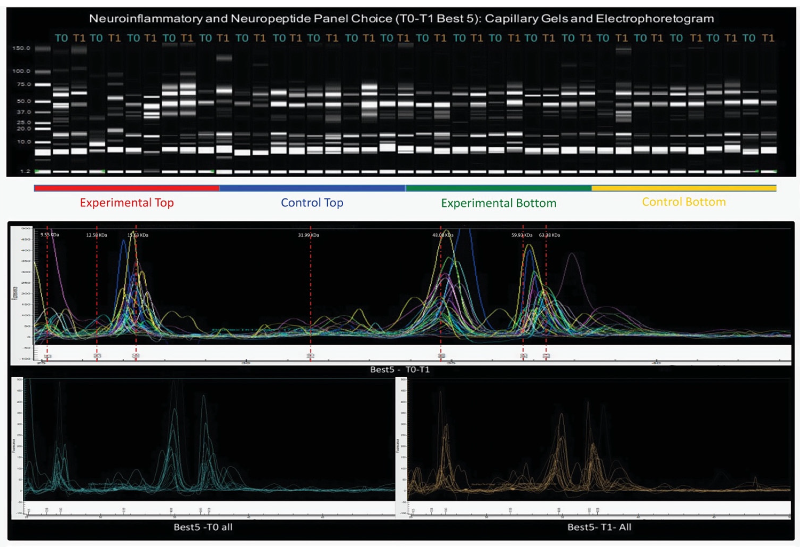
Figure 5 shows all four subgroups’ capillary gels and electropherograms of the five chosen subjects for the neuroinflammatory and neuropeptide panel.

All subjects (from all the subgroups) in T0 + T1 are plotted together, and in T0 (before) and T1 (after), the Intervention Protocol. Likewise, the capillary gel from the total four subgroups is shown separately, in T0 + T1.

In the interval I. [9.1;17] kDa, the total four subgroups of the study showed two protein peaks of a considerably high heterogeneity, both in the MW range and in fluorescence (concentration (ng/µL)), which need further investigation. Likewise, in interval II. [17;30] kDa, the total four subgroups of the study showed one protein peak of considerably high heterogeneity, more in the MW range variable than in the concentration variable.

This heterogeneity can also be observed in the capillary gels.

In Figure 6, it is possible to see the electropherograms, separately in T0 and T1, of the subjects belonging only to the (1) Experimental Top Subphenome.

Five subjects were plotted. Moreover, they were also charted together in T0 + T1 without the positive control for that group. The fourth graph shows T0 + T1 for the positive control, a subject with an ICD-10 classification: J30.1—Allergic rhinitis due to pollen and medicated with the antihistaminergic Zyrtec.

As is shown in the first two graphs, there is considerable variability from the T1 to the T0, specifically, a slight increase in the concentration (ng/µL) in the interval I. [9.1;17] kDa and a substantial decrease in the concentration (ng/µL) in the interval II. [17;30] kDa. These results confirm the hypotheses made previously in the MODeLING.Vis for the Δ (T1 − T0) ng/µL of the (B) [9.8;10.3] kDa and (D) [13.7;17.5] kDa MW range.

In the third graph, we can see the overall intragroup homogeneity of the concentration (ng/µL) in the [9.1;30] kDa (the (c) lower MW range), contrastingly to the positive control, plotted in the fourth graph, showing a significant increase in the concentration in this MW range.

Specifically, this augmentation is visible in interval I. [9.1;17] kDa; this augmentation is visible in interval I. [9.1;17] kDa.

In Figure 7, the same electropherograms are equally shown, but for the five subjects belonging to (3) the Experimental Bottom Subphenome.

In this case, the fourth graph shows T0 + T1 for the positive control, a subject with an ICD 10: J30.9—Allergic Rhinitis, unspecified and nonmedicated.

As is shown in the first two graphs, there is considerable variability from T1 to T0, specifically a significant increase in the concentration (ng/µL) of both intervals I. [9.1;17] kDa and II. [17;30] kDa. In this electropherogram, the atypical protein profile is due to the positive control in the [9.1;17] kDa, and is better demonstrated in the fourth graph, showing a significant decrease in the concentration in this MW range.

These results also confirm the hypothesis made previously in the MODeLING.Vis for the Δ (T1 − T0) ng/µL of the (B) [9.8;10.3] kDa and (D) [13.7;17.5] kDa MW range.

In the third graph, we can also see the overall intragroup homogeneity of the concentration in the [9.1;30] kDa, contrasting with the positive control, plotted in the fourth graph.

Figure 8 shows the five subjects belonging to the (2) Control Top Subphenome. In this situation, the fourth graph shows T0 + T1 for the positive control, a subject with an ICD-10: J45—Asthma, nonmedicated.

As is shown in the first two graphs, there is considerable variability from T1 to T0, specifically a slight decrease in the concentration (ng/µL) in both intervals I. [9.1;17] kDa and II. [17;30] kDa.

These results also confirm the hypothesis made previously in the MODeLING.Vis for the Δ (T1 − T0) ng/µL of the (B) [9.8;10.3] kDa and (D) [13.7;17.5] kDa MW range. In the third graph, we can see the overall intragroup homogeneity of the concentration in the [9.1;30] kDa.

Additionally, the electropherogram of the positive control, plotted in the fourth graph, shows a baseline control concentration in interval II. [17;30] kDa, characteristic of the neuroinflammatory response.

Figure 9 shows the five subjects belonging to the (4) Control Bottom Subphenome. In this condition, the fourth graph shows T0 + T1 for the positive control, which was a subject with an ICD-10: J30.9—Allergic Rhinitis, unspecified, and medicated with a leukotriene receptor antagonist (Singulair^®), a corticosteroid (Pulmicort^®), and a long-acting β2-agonist (Simbicort^®).

As shown in the first two graphs, there is considerable variability from T1 to T0, specifically the significant concentration increase (ng/µL) in interval II. [17;30] kDa.

These results also confirm the hypothesis made previously in the MODeLING.Vis for the Δ (T1 − T0) ng/µL of the B) [9.8;10,3] kDa (which remains constant) and D) [13.7;17.5] kDa (which augments considerably) MW range. The third graph shows a slight overall intragroup heterogeneity in the [9.1;30] kDa MW range compared to the other subgroups.

This heterogeneity is due to the lower clinical score characterizing this subgroup [17] and, therefore, lower specific molecular print in this MW range.

The electropherogram of the positive control, plotted in the fourth graph, shows a baseline control concentration in interval II. [17;30] kDa, which is also characteristic of the neuroinflammatory response.

After this analysis, we postulate that those five subjects should be chosen to advance for a sequential phase of our molecular screening: simultaneous immune detection.

The excerpt of the research outline (Figure 10) systemizes the experimental study and helps the reader understand this paper’s sequence and integration in the overall experiment conducted by the authors.

4. Discussion

The total protein profile acquired usually lacks adequate resolution for analyte quantification compared to high-throughput techniques, such as nanoliquid chromatography–tandem mass spectrometry. Indeed, acquiring data with the Experion^TM automated electrophoresis system (Biorad^®, Bio-Rad Laboratories, Inc., Hercules, California, USA) offers a low capacity to discriminate individual proteins and specific MW bands. This low capacity influences the electrophoretic patterns, characterized by a conjunction of proteins that migrate to the same MW and not to a particular and single protein migration.

Moreover, the electrophoretic bands usually have an associated error corresponding to the lack of accuracy offered by Experion^TM analysis; and what is seen in a MW band should account for this inaccuracy related to the instrument and measure. Consequently, for the reasons presented above and to ensure precise quantification and discriminative power, a multiplexed simultaneous immune detection was proposed and used in a sequential phase of this experiment.

Henceforward, and considering the limitations of this electrophoresis-based technique, we proposed using a MATLAB GUI toolbox to set viable hypotheses and to design possible conclusions. The objective was not to compare an electrophoresis-based approach with high-resolution methods such as mass spectrometry (accurate proteomics data), which would not be reliable, but risky and unfounded.

Taking this concern with much care, we combined, Experion^TM and MATLAB, offering a more effective methodological strategy. This strategy was only used as an initial qualitative top-down approach for stratifying four molecular profiles in neurotypical subjects.

Previous mental health stratification in this experiment had already obtained those profiles. That mental health stratification permitted the choice of the subjects that better represented each subgroup and, therefore, were potentially better candidates for a specific protein profile. Combined Experion^TM and MATLAB analysis advanced with the possibility of further characterizing cognition with a preliminary low-end molecular technique. Moreover, this analysis also offered the consequent hypothesis of quantifying those four mental health–molecular profiles with better discriminative power.

We stress that as descriptive research, the central hypothesis of this study was centered mainly on its methodology strategies, to take full benefit from the limited financial funds for the experiment and the restraints of using an electrophoresis-based technique versus high-resolution methods such as mass spectrometry. With this chief limitation in mind, primary outcomes were already attained in a previous publication: (i) the pipeline identification of neuronal–saliva protein profiles and (ii) the protein stratification of neurotypical young adults. With this publication, we concluded (iii) the GUI toolbox development for data visualization of those strata, and (iv) the selection of subjects advancing for quantification.

MODeLING.Vis permitted adequate data mining of limited neuroproteomics datasets. This data mining consisted of both unsupervised/unlabeled and supervised/labeled machine learning. Initially, the subjects were imported, and no labels were given to the learning algorithm, leaving it on its own to find structure in its input. Later, in a posterior phase of the data mining, the subjects were labeled to compare individual subjects’ protein concentration (ng/µL) in specific MW intervals.

Initially, all the subgroups’ protein profiles, comprising all electrophoretic runs, were systematically and randomly uploaded to the algorithms. The algorithms then performed an exploratory data analysis, discovering hidden patterns in protein profile data. A first dataset, i.e., total protein profiles, was inputted for feature learning of functional protein network profiles.

Until now, as a limitation, only capillary electrophoresis data had been explored, but this GUI toolbox is also designed for other datasets, for instance, multiplex simultaneous immunodetection. Likewise, this GUI toolbox allows further integration of the acquired psychological data, the intersubjective mental health profile [17]. Only relying on standard methods for analyzing those databases (e.g., assessment of the covariance between variables) might provide suboptimal results due to the high number of measured quantities and possible nonlinear relationships [51] among them.

The datasets generated by this full cognitive–molecular study should optimally be intercorrelated in a phenomic multidata approach. Hence, our data mining solution was planned to discover and model patterns, for instance, the EM algorithm used to find the MW intervals shown in Figure 11.

Data visualization techniques were adopted for the molecular profiles’ interactive query (Figure 12). This interactive query of the acquired Experion^TM Protein Profile data offered the chance to check for functional network profiles.

Moreover, it also showed the whole effort of the authors to find differences in the electrophoretic separation by Experion^TM in the different samples, facing the limitations of a system that prevents the extraction of direct and solid conclusions.

Finally, and for that matter, data classification and regression algorithms are being devised for operational applications, such as recognizing a molecular state or profile from the analysis of salivary samples. Expectantly, the same regression algorithms will also be used in the future to recognize a mental health state or trait from the analysis of the molecular profiles.

To summarize, three central components were defined: data visualization, data exploration, and the development of algorithms. These components encompassed a data mining toolbox, which aimed to:

(i) Implement and test visualization software that allowed the interactive exploratory of information content embedded in multilayered and multisource data;

(ii) Service the scientific community by distributing, instructing, and supporting software users, i.e., researchers and clinicians.

The results of this investigation moderately emphasized the molecular strategy we developed for identifying functional networks as a complementary and alternative method in neurobiology.

We applied the FAIR data principles to the electrophoretic data of the pipeline oral proteome study and the full approach on the 92 neurotypical young adults. Likewise, FAIR principles were maintained in the data mining by the expectation–maximization (EM) algorithm and the GUI toolbox.

The digital research objects [52], from the electrophoretic data to the analytical pipelines offered by MODeLING.Vis, ensured transparency, reproducibility, and reusability.

Hence, a follow-up molecular study of a selected sample is proposed for further proteomic explorations and quantification. This follow-up study can better characterize the molecular substrates of the neurotypical development of young adults, as it probes into the neuropeptide and neuroinflammatory response with a high-resolution method.

For now, and with the limited internal validity offered by low-end techniques, we can only conclude that the neurotypical phenome is a complex result of the intercorrelation of mental health [17] and the consequent expression of protein networks.

Those protein networks, generated in the brain, may be detected in saliva and usually correspond to small neuroimmune molecules or neuropeptides crossing the blood-brain barrier.

Finally, the [9.1;30] kDa molecular weight range should be better quantified when studying a neurotypical sample because it offers a possible solution for probing into the neurocognitive response.

Please note that an error variable should be considered and correspond to the lack of accuracy offered by ExperionTM analysis and the identified MW ranges.

These considerations should take this inaccuracy into account, but also the process of protein degradation observed and well documented in saliva.

MODeLING.Vis: FAIR Principles for Scientific Data Management, Video Tutorial, and Stand-Alone Executable

In analyzing our digital objects, i.e., proteomic data, we used a well-curated and deeply integrated UniProt repository [53]. UniProt is constantly curating and capturing high-value reference datasets on proteins and fine-tuning them to enrich scholarly outputs, delivering comprehensive tools to access their dynamic protein data.

Moreover, we also shared our data with the community by using the open globally-scoped repository named Zenodo (http://zenodo.org/ (accessed on 23 November 2022)) for “EPPStrategyDataExport” (https://0-doi-org.brum.beds.ac.uk/10.5281/zenodo.7054406, accessed on 20 November 2022), “ExportForMOdeLINGVis” (https://0-doi-org.brum.beds.ac.uk/10.5281/zenodo.7054551, accessed on 22 November 2022), and MODeLING.Vis (https://0-doi-org.brum.beds.ac.uk/10.5281/zenodo.7041477, accessed on 21 November 2022).

In our study’s descriptive research, Zenodo was used as a preliminary repository of data, but to avoid the decentralization of our datasets and the reusability problem, in the future, we will publish our explanatory analysis in special-purpose repositories for the life sciences, such as Genbank [54], Worldwide Protein Data Bank [55], or UniProt.

MODeLING.Vis was designed as an attempt to perform interactive data analyses. Given the software’s effectiveness in extracting valuable information from the experimental data presented in this study, the applied methods and principles have been presented together with the analysis of results, and the code has been shared.

Note, however, that MODeLING.Vis is not commercial, which constrains efforts behind scientific investigations. In order to provide a demo/user manual for the MODeLING.Vis toolbox for users’ convenience, we created a video tutorial demonstrating how to download, install, run, and operate MODeLING.Vis.

The practical video tutorial can be accessed online and was attributed a https://0-doi-org.brum.beds.ac.uk/10.5281/zenodo.7337428 (accessed on 30 November 2022). The electrophoretic dataset (protLabled.xls) is published together with the tutorial for ease of access.

Concerning the creation of a MODeLING.Vis stand-alone executable or compiled .exe file from the MATLAB code file, it requires additional efforts on the users’ side, such as downloading and installing a run-time MATLAB library.

In its turn, this could create drawbacks when software updates are needed, and compatibility between the runtime library and the executable is required. Henceforth, a MODeLING.Vis stand-alone executable would go behind the possibilities of the present study.

5. Conclusions

The paper tested a symmetric correlation between the psychological data offered by the mental health stratification already published by the authors [17,18,19] and the molecular data offered by capillary electrophoresis.

To better correlate both mental health and total protein profiles, a GUI toolbox was developed—MODeLING.Vis (Figure 13, https://0-doi-org.brum.beds.ac.uk/10.5281/zenodo.7041477, accessed on 21 November 2022).

Hence, MODeLING.Vis permitted to address the problem of the low discriminative power of capillary electrophoresis and offered:

i. Data visualization by a graphical user interface toolbox, using expectation–maximization (EM) iteration, which depends on unobserved latent variables.

ii. Data exploration by hypothesis testing of the biomolecular data. Moreover, the toolbox is prepared to integrate other neuromolecular datasets.

iii. Data mining of the acquired neuroproteomics data, comparing individual molecular profiles to the whole sample.

In order to give a brief explanation of the structure of the GUI toolbox, a flow chart (Figure 14) summarizes the ten processing steps executed in MATLAB.

In the first step, the acquired full protein profile by capillary electrophoresis (Experion™ Automated System, Biorad^®) was imported.

In the second step, the accurate m/z value for each peak detected within the time domain was calculated with a Gaussian curve-fitting m/z domain peak.

Using the EM algorithm, in the third step, the toolbox made the alignment of peaks in multiple measurements, and for the fourth step, it detected the representative peaks and MW range intervals.

In the fifth step, data distribution was performed by Gaussian mixture modeling with a set of Gaussian bell curves. Each Gaussian mixture component’s mean and standard deviation express its location and width. The weights of each bell curve are defined as an additional GMM parameter set.

In step six, data visualization was achieved by fitting the data iteratively by tuning the weights based on the mean and the standard deviation values of each Gaussian (Expectation step), and in step seven, by relying on the computed weights to update the mean and the standard deviation values (Maximization step).

The data mining of electropherograms was achieved: in step 8, by identifying corresponding peaks across multiple samples; in step 9, by optimizing the numerical parameters of the normalization function; and in step 10, by quantifying the molecular subphenomes. Thus, MODeLING.Vis used unsupervised and supervised machine learning and facilitated the exploration of the acquired electrophoretic data with a low-end method and low-cost technique. Our electrophoretic dataset can be quickly and automatically integrated with private in-house data and with other third-party protein data repositories. In our investigation and the future publications of the authors, we privileged UniProt as it is a wide-ranging resource for protein sequence and annotation data, where all entries are exclusively identified by a stable URL. The protein record offered contains rich metadata using shared vocabularies and ontologies. Moreover, each UniProt record interacts with different databases, such as PubMed, enabling rich citation and permitting cross-referencing of our neuroproteomics data.

Finally, the outcome of that descriptive analysis was hypothesizing the [9.1;30] kDa molecular weight range as an interesting molecular range for adequate quantification. This MW range, obtained by pattern recognition of our dataset, has been published as characteristic of small neuroimmune molecules and neuropeptides and thus offers a possible solution for probing into the neurocognitive response.

MODeLING.Vis: Limitations and Future Scope

In summary, MODeLING.Vis provides three main functions: data visualization, exploration, and mining. In this paper, MODeLING.Vis is used to analyzing electrophoretic data of neurotypical young adults. Expectation–maximization (EM) iteration provides data visualization of the electrophoretic profiles to explore unobserved latent variables in our dataset.

MODeLING.Vis also executes data mining of our dataset, comparing individual molecular profiles to the whole sample, and permits better visualization of the homogeneous separation of the salivary peptides.

MODeLING.Vis accepts a T1 − T0 variate input threshold (ng/µL) defined by the researcher to explore T1 − T0 electrophoretic differences better. As shown in Figure 4, this variate input threshold is used to compare the electrophoretic profile between subjects, for example, between the Experimental Top subgroup (in red, subject D01383) and other subgroups. Likewise, MODeLING.Vis permits the better visualization of intersubject differences by plotting data clusters in three PCA components with statistical relevance (p < 0.05).

In a further publication, the authors will publish an extended electrophoretic analysis of both the pipeline oral proteome study and the full approach on the 92 neurotypical young adults. This subsequent paper will plot and illustrate the total protein profiles of the 92 subjects as an innovative probe using saliva. Subsequently, the authors show that the 92 young adults showed specific expected protein profiles present in saliva, which correspond to the four psychologically different subgroups (self-awareness, self-consciousness, reflective self, and pre-reflective self) found in the neurotypical subjects with discrete self-processes [56].

However, MODeLING.Vis is a GUI toolbox used for common unsupervised and/or supervised machine learning and can be generalized and extrapolated to other samples and populations. Moreover, MODeLING.Vis is prepared to integrate other neuromolecular datasets. For example, in a future study, the authors will use MODeLING.Vis not only to select the most representative electrophoretic molecular profiles but also for data exploration of combined neuropeptide and neuroimmune panels. Thus, MODeLING.Vis is already designed to integrate other molecular panels obtained by simultaneous immunodetection, which the authors will use for the data exploration of neuropeptides and messengers of the neuroimmune response.

Instead, these neuromolecular datasets will be obtained by a combined multiplex panel: the Human Neuropeptide Assay, [9.1;17] kDa, and the Human Th17 Cytokine Assay, [17;30] kDa. In this case, MODeLING.Vis will permit the identification of subgroups in a sample of neurotypical young adults with a homogeneous molecular profile consistent with the neuropeptide and neuroimmune response. The analysis of this profile of analytes, comprising 19 molecules with distinct concentrations (pg/mL) in our four molecular subphenomes, will permit, as an outcome, the preliminary identification of possible biomarkers of susceptibility in neurotypical young adults.

The outcome of this study is thus to correlate the four different mental health strata [17,56] with the four different molecular profiles using MODeLING.Vis as a GUI toolbox. The practical proposition of this analysis is to accomplish the molecular assessment of self-regulation processes with separate cognitive and molecular characteristics. The reliability of these mental–molecular strata and their distinct neuropsychophysiology will be tested in future publications of the same participants.

In conclusion, this analysis precedes explanatory and causalistic analysis but may be used for other design studies in neuroproteomics and the screening and monitoring of neurodevelopmental disorders. The authors plan, in the future, to test MODeLING.Vis with a neurodevelopmental cohort of patients. Henceforth, MODeLING.Vis can also be used to study a sample of patients with autism spectrum disorder, intellectual disability, or other neurogenetic diseases, for example, Fragile X, Prader–Willi, Phelan–McDermid, and Rett’s syndromes.

References

1. Esteves, E.; Fernandes, M.; Cruz, I.; Esteves, F.; Rosa, N.; Correia, M.J.; Barros, M. Saliva Print: Sheep saliva electrophoretic protein profile in a bioinformatics approach. Cut. Edge Pathol. 2017, 2017, 74. [Google Scholar]
2. Saavedra Silva, M.; Sousa, S.; Silva, A.; Martins, J.E.; Esteves, E.; Fernandes, M.; Rosa, N.; Correia, M.J.; Barros, M. Salivary Protein Profile as a Tool for Patient Stratification in Peri-Implantitis; ITI World Symposium: Basel, Switzerland, 2017. [Google Scholar] [CrossRef]
3. Henson, R.; Cetto, L. The MATLAB bioinformatics toolbox. In Encyclopedia of Genetics, Genomics, Proteomics and Bioinformatics; Wiley: Hoboken, NJ, USA, 2005. [Google Scholar]
4. Kim, J.H.; Kim, Y.W.; Kim, I.W.; Park, D.C.; Kim, Y.W.; Lee, K.H.; Ahn, W.S. Identification of candidate biomarkers using the Experion™ automated electrophoresis system in serum samples from ovarian cancer patients. Int. J. Oncol. 2013, 42, 1257–1262. [Google Scholar] [CrossRef] [PubMed] [Green Version]
5. Thakur, N.; Han, C.Y. A study of fall detection in assisted living: Identifying and improving the optimal machine learning method. J. Sens. Actuator Netw. 2021, 10, 39. [Google Scholar] [CrossRef]
6. Pande, S.; Kamparia, A.; Gupta, D. Recommendations for DDOS Threats Using Tableau. In Proceedings of Data Analytics and Management; Springer: Singapore, 2022; pp. 73–84. [Google Scholar]
7. Bishop, C.M. Neural Networks for Pattern Recognition; Oxford University Press: Oxford, UK, 1995. [Google Scholar]
8. Nabney, I. NETLAB: Algorithms for Pattern Recognition; Springer Science & Business Media: Berlin, Germany, 2002. [Google Scholar]
9. Kumar, R.; Singh, S.; Dubey, V.K. Bioinformatics Tools to Analyze Proteome and Genome Data. In Advances in the Understanding of Biological Sciences Using Next Generation Sequencing (NGS) Approaches; Springer: Cham, Switzerland, 2015; pp. 179–194. [Google Scholar]
10. Ottman, N.; Davids, M.; Suarez-Diez, M.; Boeren, S.; Schaap, P.J.; dos Santos, V.A.M.; de Vos, W.M. Genome-scale model and omics analysis of metabolic capacities of Akkermansia muciniphila reveal a preferential mucin-degrading lifestyle. Appl. Environ. Microbiol. 2017, 83, e01014-17. [Google Scholar] [CrossRef] [Green Version]
11. Hou, C.; Li, Y.; Liu, H.; Dang, M.; Qin, G.; Zhang, N.; Chen, R. Profiling the interactome of protein kinase C ζ by proteomics and bioinformatics. Proteome Sci. 2018, 16, 5. [Google Scholar] [CrossRef] [Green Version]
12. Cruz, I.; Esteves, E.; Fernandes, M.; Martins, J.E.; Silva, M.; Sousa, S.; Rosa, N.; Correia, M.J.; Arrais, J.P.; Barros, M. Bringing Saliva into Research—SalivaPrint, Algorithms and Personalized Medicine; Science 2017; Science and Technology Foundation: Lisbon, Portugal, 2017. [Google Scholar]
13. Cruz, I.; Esteves, E.; Fernandes, M.; Rosa, N.; Correia, M.J.; Arrais, J.P.; Barros, M. Saliva PRINT Toolkit–Protein profile evaluation and phenotype stratification. J. Proteom. 2018, 171, 81–86. [Google Scholar] [CrossRef]
14. Sultana, R.; Perluigi, M.; Newman, S.F.; Pierce, W.M.; Cini, C.; Coccia, R.; Butterfield, D.A. Redox proteomic analysis of carbonylated brain proteins in mild cognitive impairment and early Alzheimer’s disease. Antioxid. Redox Signal. 2010, 12, 327–336. [Google Scholar] [CrossRef] [Green Version]
15. Weyl, H. Symmetry. J. Wash. Acad. Sci. 1938, 28, 253–271. [Google Scholar]
16. Odintsov, S.D.; Paul, T.; Banerjee, I.; Myrzakulov, R.; SenGupta, S. Unifying an asymmetric bounce to the dark energy in Chern–Simons F (R) gravity. Phys. Dark Universe 2021, 33, 100864. [Google Scholar] [CrossRef]
17. Hipólito, I.; Martins, J. Mind-life continuity: A qualitative study of conscious experience. Prog. Biophys. Mol. Biol. 2017, 131, 432–444. [Google Scholar] [CrossRef] [Green Version]
18. Martins, J.E.; Simões, M.; Rosa, N.; D’Alimonte, D.; Mendes, V.M.; Correia, M.J.; Barros, M.; Manadas, B. Happiness as a self state and trait of consciousness: Saliva molecular biomarkers—A brief revision. Exp. Pathol. Health Sci. Res. Clin. Teach. Soc. 2016, 8, 51–54. [Google Scholar]
19. Martins, J.E.; Simões, M.; Ferreira, H.; Tavares, V.; Brito, J.; Carvalho, L.X.; Carvalho, E.N.; Castelo-Branco, M. Self-reflexive consciousness: A model for the experimental use of neurofeedback in sensorial immersion in a center for consciousness knowledge. Exp. Pathol. Health Sci. Res. Clin. Teach. Soc. 2016, 8, 55–58. [Google Scholar]
20. Newell, D.B.; Tiesinga, E. The International System of Units (SI); NIST Special Publication: Gaithersburg, MD, USA, 2019; Volume 330, pp. 1–138. [Google Scholar]
21. Helmenstine, A.M. Molecular Weight Definition; Tennessee at Knoxville: Knoxville, Tennessee, 2014. [Google Scholar]
22. Wilkinson, M.; Dumontier, M.; Aalbersberg, I.; Appleton, G.; Axton, M.; Baak, A.; Blomberg, N.; Boiten, J.W.; da Silva Santos, L.B.; Bourne, P.E.; et al. The FAIR Guiding Principles for scientific data management and stewardship. Sci. Data 2016, 3, 160018. [Google Scholar] [CrossRef]
23. Hirayama, A.; Kami, K.; Sugimoto, M.; Sugawara, M.; Toki, N.; Onozuka, H.; Soga, T. Quantitative metabolome profiling of colon and stomach cancer microenvironment by capillary electrophoresis time-of-flight mass spectrometry. Cancer Res. 2009, 69, 4918–4925. [Google Scholar] [CrossRef] [Green Version]
24. Minami, Y.; Kasukawa, T.; Kakazu, Y.; Iigo, M.; Sugimoto, M.; Ikeda, S.; Ueda, H.R. Measurement of internal body time by blood metabolomics. Proc. Natl. Acad. Sci. USA 2009, 106, 9890–9895. [Google Scholar] [CrossRef] [Green Version]
25. Saito, N.; Robert, M.; Kochi, H.; Matsuo, G.; Kakazu, Y.; Soga, T.; Tomita, M. Metabolite profiling reveals YihU as a novel hydroxybutyrate dehydrogenase for alternative succinic semialdehyde metabolism in Escherichia coli. J. Biol. Chem. 2009, 284, 16442–16451. [Google Scholar] [CrossRef] [Green Version]
26. Smith, C.A.; Want, E.J.; O’Maille, G.; Abagyan, R.; Siuzdak, G. XCMS: Processing mass spectrometry data for metabolite profiling using nonlinear peak alignment, matching, and identification. Anal. Chem. 2006, 78, 779–787. [Google Scholar] [CrossRef] [PubMed]
27. Baran, R.; Kochi, H.; Saito, N.; Suematsu, M.; Soga, T.; Nishioka, T.; Tomita, M. Math DAMP: A package for differential analysis of metabolite profiles. BMC Bioinform. 2006, 7, 530. [Google Scholar] [CrossRef] [Green Version]
28. Soga, T.; Baran, R.; Suematsu, M.; Ueno, Y.; Ikeda, S.; Sakurakawa, T.; Tomita, M. Differential metabolomics reveals ophthalmic acid as an oxidative stress biomarker indicating hepatic glutathione consumption. J. Biol. Chem. 2006, 281, 16768–16776. [Google Scholar] [CrossRef] [Green Version]
29. Wallace, W.E.; Kearsley, A.J.; Guttman, C.M. An operator-independent approach to mass spectral peak identification and integration. Anal. Chem. 2004, 76, 2446–2452. [Google Scholar] [CrossRef]
30. Reijenga, J.C.; Martens, J.H.; Giuliani, A.; Chiari, M. Pherogram normalization in capillary electrophoresis and micellar electrokinetic chromatography analysis in cases of sample matrix-induced migration time shifts. J. Chromatogr. B 2002, 770, 45–51. [Google Scholar] [CrossRef] [PubMed]
31. Starr, J.; Castro, E.; Crosas, M.; Dumontier, M.; Downs, R.R.; Duerr, R.; Clark, T. Achieving human and machine accessibility of cited data in scholarly publications. PeerJ Comput. Sci. 2015, 1, e1. [Google Scholar] [CrossRef] [PubMed] [Green Version]
32. Do, C.B.; Batzoglou, S. What is the expectation-maximization algorithm? Nat. Biotechnol. 2008, 26, 897. [Google Scholar] [CrossRef] [PubMed]
33. Banks, W.A. Characteristics of compounds that cross the blood-brain barrier. In BMC Neurology; BioMed Central: London, UK, 2009; Volume 9, p. S3. [Google Scholar]
34. Pardridge, W.M. Blood-brain barrier delivery. Drug Discov. Today 2007, 12, 54–61. [Google Scholar] [CrossRef] [PubMed]
35. Salameh, T.S.; Banks, W.A. Delivery of therapeutic peptides and proteins to the CNS. In Advances in Pharmacology; Academic Press: Cambridge, MA, USA, 2014; Volume 71, pp. 277–299. [Google Scholar]
36. Banks, W.A. Peptides and the blood-brain barrier. Peptides 2015, 72, 16–19. [Google Scholar] [CrossRef] [Green Version]
37. De Vries, H.E.; Kuiper, J.; de Boer, A.G.; Van Berkel, T.J.; Breimer, D.D. The blood-brain barrier in neuroinflammatory diseases. Pharmacol. Rev. 1997, 49, 143–156. [Google Scholar]
38. Erickson, M.A.; Banks, W.A. Neuroimmune Axes of the Blood-Brain Barriers and Blood-Brain Interfaces: Bases for Physiological Regulation, Disease States, and Pharmacological Interventions. Pharmacol. Rev. 2018, 70, 278–314. [Google Scholar] [CrossRef] [Green Version]
39. Fregonese, L.; Stolk, J. Hereditary alpha-1-antitrypsin deficiency and its clinical consequences. Orphanet J. Rare Dis. 2008, 3, 1–9. [Google Scholar] [CrossRef] [Green Version]
40. Desai, S.; Ding, M.; Wang, B.; Lu, Z.; Zhao, Q.; Shaw, K.; Yao, J. Tissue-specific isoform switch and DNA hypomethylation of the pyruvate kinase PKM gene in human cancers. Oncotarget 2014, 5, 8202. [Google Scholar] [CrossRef] [Green Version]
41. Sun, J.; Axelsson, J.; Machowska, A.; Heimbürger, O.; Bárány, P.; Lindholm, B.; Qureshi, A.R. Biomarkers of cardiovascular disease and mortality risk in patients with advanced CKD. Clin. J. Am. Soc. Nephrol. 2016, 11, 1163–1172. [Google Scholar] [CrossRef] [PubMed] [Green Version]
42. Rosa, N.; Correia, M.J.; Arrais, J.P.; Lopes, P.; Melo, J.; Oliveira, J.L.; Barros, M. From the salivary proteome to the OralOme: Comprehensive molecular oral biology. Arch. Oral Biol. 2012, 57, 853–864. [Google Scholar] [CrossRef] [PubMed]
43. Arrais, J.P.; Rosa, N.; Melo, J.; Coelho, E.D.; Amaral, D.; Correia, M.J.; Oliveira, J.L. OralCard: A bioinformatics tool for the study of oral proteome. Arch. Oral Biol. 2013, 58, 762–772. [Google Scholar] [CrossRef]
44. Wilson, M.E.; Boumaza, I.; Bowser, R. Measurement of cystatin C functional activity in the cerebrospinal fluid of amyotrophic lateral sclerosis and control subjects. Fluids Barriers CNS 2013, 10, 15. [Google Scholar] [CrossRef] [PubMed] [Green Version]
45. Aureli, A.; Sebastiani, P.; Del Beato, T.; Marimpietri, A.E.; Graziani, A.; Sechi, E.; Di Loreto, S. Involvement of IL-6 and IL-1 receptor antagonist on intellectual disability. Immunol. Lett. 2014, 162, 124–131. [Google Scholar] [CrossRef]
46. Suzumura, A.; Ikenaka, K. (Eds.) Neuron-Glia Interaction in Neuroinflammation; Springer Science & Business Media: Berlin, Germany, 2013; Volume 7. [Google Scholar]
47. Wang, Y.; Wang, M.; Yin, S.; Jang, R.; Wang, J.; Xue, Z.; Xu, T. NeuroPep: A comprehensive resource of neuropeptides. Database 2015, 2015, bav038. [Google Scholar] [CrossRef] [PubMed] [Green Version]
48. Young, A.M.; Chakrabarti, B.; Roberts, D.; Lai, M.C.; Suckling, J.; Baron-Cohen, S. From molecules to neural morphology: Understanding neuroinflammation in autism spectrum condition. Mol. Autism 2016, 7, 9. [Google Scholar] [CrossRef] [PubMed] [Green Version]
49. Lim, M.M.; Bielsky, I.F.; Young, L.J. Neuropeptides and the social brain: Potential rodent models of autism. Int. J. Dev. Neurosci. 2005, 23, 235–243. [Google Scholar] [CrossRef]
50. Hipólito, I.; Martins, J.E. A “Second-Person” Model to Anomalous Social Cognition. In Schizophrenia and Common Sense; Hipólito, I., Gonçalves, J., Pereira, J., Eds.; Studies in Brain and Mind; Springer: Cham, Switzerland, 2018; Volume 12. [Google Scholar]
51. D’Alimonte, D.; Lowe, D.; Nabney, I.T.; Mersinias, V.; Smith, C.P. MILVA: An interactive tool for the exploration of multidimensional microarray data. Bioinformatics 2005, 21, 4192–4193. [Google Scholar] [CrossRef] [Green Version]
52. Bechhofer, S.; De Roure, D.; Gamble, M.; Goble, C.; Buchan, I. Research objects: Towards exchange and reuse of digital knowledge. Nat. Preced. 2010, 1, 1. [Google Scholar] [CrossRef]
53. Consortium, U. UniProt: A hub for protein information. Nucleic Acids Res. 2015, 43, D204–D212. [Google Scholar] [CrossRef] [Green Version]
54. Benson, D.A.; Cavanaugh, M.; Clark, K.; Karsch-Mizrachi, I.; Ostell, J.; Pruitt, K.D.; Sayers, E.W. GenBank. Nucleic Acids Res. 2018, 46, D41–D47. [Google Scholar] [CrossRef] [PubMed] [Green Version]
55. Berman, H.; Henrick, K.; Nakamura, H. Announcing the worldwide protein data bank. Nat. Struct. Mol. Biol. 2003, 10, 980. [Google Scholar] [CrossRef] [PubMed]
56. Martins, J.E.; Simões, J.; Barros, M.; Simões, M. Pre-Molecular Assessment of Self-Processes in Neurotypical Subjects Using a Single Cognitive Behavioral Intervention Evoking Autobiographical Memory. Behav. Sci. 2022, 12, 381. [Google Scholar] [CrossRef] [PubMed]
Figure 1. MODeLING.Vis Data Visualization: use of the MODeLING.Vis with EM iteration, delimiting the concentration (ng/µL) thresholds and the quantity of MW intervals (kernels = 13). It provides the identification of the following significant (p < 0.05) intervals of MW: (A) [9.1;9.8] kDa, (B) [9.8;10.3] kDa, (C) [10.3;13.7] kDa, (D) [13.7;17.5] kDa, (E) [17.5;21.1] kDa, (F) [21.1;24.7] kDa, (G) [24.7;36] kDa, (H) [36;42.6] kDa, (I) [42.6;51.5] kDa, (J) [51.5;65] kDa, (K) [65;77] kDa, and (L) [77;149.7] kDa.
Symmetry 15 00042 g001
Figure 2. MODeLING.Vis Data Exploration T0: an exploration of the electrophoretic dataset for T0, defining the threshold to 2500 ng/µL. Experimental Top is shown in red, Experimental Bottom is shown in green, Control Top is shown in blue, and Control Bottom is shown in yellow. Data clusters in only two PCA components are represented. A small but not significant (p > 0.05) separation of the Experimental Top (red square) and Control Bottom (yellow circle) subgroups are presented.
Symmetry 15 00042 g002
Figure 3. MODeLING.Vis Data Exploration T1: an exploration of the electrophoretic dataset for T1, defining the threshold to 2500 ng/µL. The Experimental Top is shown in red, Experimental Bottom is shown in green, Control Top is shown in blue, and Control Bottom is shown in yellow. Data clusters in three PCA components are represented. A more relevant separation of the Experimental Top (red square) and Control Bottom (yellow circle) subgroups (when compared to T0) is presented.
Symmetry 15 00042 g003
Figure 4. MODeLING.Vis Data Exploration T1 − T0: an exploration of the electrophoretic dataset for T1 − T0, defining the threshold to 2500 ng/µL. Experimental Top is shown in red, Experimental Bottom is shown in green, Control Top is shown in blue, and Control Bottom is shown in yellow. Data clusters in three PCA components are represented. A significant separation (p < 0.05) of the square symbols (Experimental subgroups), distributed along the top 2PCA and 3PCA axis, and the circle symbols (Control subgroups), distributed along the bottom 2PCA and bottom 1PCA axis, is presented with statistical relevance. As an example of the statistical separation between the electropherograms of each subgroup, the image shows a comparison of the electrophoretic profiles of the subject D01383 (Experimental Top subgroup (1)), subject D01371 (Experimental Bottom subgroup (3)), subject D01337 (Control Top subgroup (2)) and subject D01319 (Control Bottom subgroup (4)).
Symmetry 15 00042 g004
Figure 5. Capillary gels and electropherogram profile of the selected best five subjects in all T0 − T1, all in T0, and all in T1, for the neuroinflammatory and neuropeptide panel. From each subphenome, for both the expected protein profile in T0, after the intervention protocol in T1, and the combined T0T1, a graphical representation is presented showing the best five capillary gels and quantitative electropherograms for the study of the neuroinflammatory and neuropeptide panel. The intergroup difference and the protein distribution are represented.
Symmetry 15 00042 g005
Figure 6. Electropherogram profile of the selected best five subjects from the Experimental Top subgroup, in T0, in T1, in T0 − T1 without positive control, and in T0 − T1 with only positive control, for the neuroinflammatory/neuropeptide panel. For the expected protein profile in T0, after the intervention protocol in T1, the combined T0T1 without the positive control, and the combined T0T1 of only the positive control, a graphical representation is presented showing the best five quantitative electropherograms of the Experimental Top subgroup to study the neuroinflammatory and neuropeptide panel. Through this figure, the intragroup difference between T0 and T1 is demonstrated.
Symmetry 15 00042 g006
Figure 7. Electropherogram profile of the selected best five subjects from the Experimental Bottom subgroup, in T0, in T1, in T0 − T1 without positive control, and in T0 − T1 only positive control, for the neuroinflammatory/neuropeptide panel. For the expected protein profile in T0, after the intervention protocol in T1, the combined T0T1 without the positive control, and the combined T0T1 of only the positive control, a graphical representation is presented showing the best five quantitative electropherograms of the Experimental Bottom subgroup to study the neuroinflammatory and neuropeptide panel. Through this figure, the intragroup difference between T0 and T1 is demonstrated.
Symmetry 15 00042 g007
Figure 8. Electropherogram profile of the selected best five subjects from the Control Top subgroup, in T0, in T1, in T0 − T1 without positive control, and in T0 − T1 only positive control, for the neuroinflammatory/neuropeptide panel. For the expected protein profile in T0, after the intervention protocol in T1, the combined T0T1 without the positive control, and the combined T0T1 of only the positive control, a graphical representation is presented showing the best five quantitative electropherograms of the Control Top subgroup to study the neuroinflammatory and neuropeptide panel. Through this figure, the intragroup difference between T0 and T1 is demonstrated.
Symmetry 15 00042 g008
Figure 9. Electropherogram profile of the selected best five subjects from the Control Bottom subgroup, in T0, in T1, in T0 − T1 without positive control, and in T0 − T1 only positive control, for the neuroinflammatory/neuropeptide panel. For the expected protein profile in T0, after the intervention protocol in T1, the combined T0T1 without the positive control, and the combined T0T1 of only the positive control, a graphical representation is presented showing the best five quantitative electropherograms of the Control Bottom subgroup to study the neuroinflammatory and neuropeptide panel. Through this figure, the intragroup difference between T0 and T1 is demonstrated.
Symmetry 15 00042 g009
Figure 10. Research outline: molecular stratification. Graphical scheme presenting the integration of this paper in the overall experiment conducted by the authors for molecular stratification of a neurotypical sample. “GUI Toolbox Development In Neurotypical Young Adults” thus considers the same methodology that led to the establishment of Neuro.SalivaPrint. It advanced with a stratification stage by data visualizing and data mining of 92 stratified subjects.
Symmetry 15 00042 g010
Figure 11. Protein profile ExperionTM data acquisition and algorithm development. Data mining solution planned to discover, and model patterns used to find the MW intervals in the neurotypical sample. A user-friendly software environment was developed to enable a thorough exploration of the information embedded in the capillary electrophoresis database.
Symmetry 15 00042 g011
Figure 12. GUI toolbox: MODeLING.Vis is used for data mining of different neuroproteomics datasets. This data mining consisted of both unsupervised/unlabeled and supervised/labeled machine learning.
Symmetry 15 00042 g012
Figure 13. MODeLING.Vis. Graphical representation of the GUI toolbox and its functions: data visualization, exploration, and mining.
Symmetry 15 00042 g013
Figure 14. MODeLING.Vis. Flow chart with a brief explanation and summary of the overall processing steps and the structure of the GUI toolbox.
Symmetry 15 00042 g014
Disclaimer/Publisher’s Note: The statements, opinions and data contained in all publications are solely those of the individual author(s) and contributor(s) and not of MDPI and/or the editor(s). MDPI and/or the editor(s) disclaim responsibility for any injury to people or property resulting from any ideas, methods, instructions or products referred to in the content.