Analytical Solutions for Fractional Differential Equations Using a General Conformable Multiple Laplace Transform Decomposition Method

Abstract

In this paper, a new analytical technique is proposed for solving fractional partial differential equations. This method is referred to as the general conformal multiple Laplace transform decomposition method. It is a combination of the multiple Laplace transform method and the Adomian decomposition method. The main theoretical results of using this method are presented. In addition, illustrative examples are provided to demonstrate the validity and symmetry of the presented method.

1. Introduction

Having attracted much attention over the last few decades due to its extensive application in almost all disciplines of applied science and engineering, fractional calculus is widely used in fractional partial differential equations (PDEs) to model problems in the real world [1,2,3,4,5,6,7,8,9,10,11,12,13,14,15,16,17,18]. Most fractional derivative definitions are the Riemann–Liouville, Caputo, and Grunwald–Letnikov definitions. However, the above fractional derivatives lack some basic properties such as the chain rule and Leibniz rule for derivatives [1].

Ref. [2] discusses some non-standard definitions of Caputo fractional derivatives and their applications as well as addressing some “fractional” analogues of the Leibniz rule.

In 2014, Khalil et al. [1,3] proposed a new definition: conformable derivative, which has the Leibniz rule and the chain rule as classic derivatives.

For the function $f:\left(0,\infty \right)\to R$, the conformable derivative of order $\alpha \in \left(0,1\right]$ of f at $x>0$ is expressed as

$$T^{\alpha }f\left(x\right)=\underset{h\to 0}{lim}\frac{f\left(x+h{x}^{1-\alpha }\right)-f\left(x\right)}{h}.$$

(1)

This new fractional derivative has both physical and geometrical interpretations [8], satisfying the following basic properties and theorems as referred to in [1,3]:

(1)

$T^{\alpha }\left(cf\left(x\right)+dg\left(x\right)\right)=c{T}^{\alpha }\left(f\left(x\right)\right)+d{T}^{\alpha }\left(g\left(x\right)\right),\forall c,d\in R;$

(2)

$T^{\alpha }\left(c\right)=0$, for all constant functions $f\left(x\right)=c;$

(3)

$T^{\alpha }\left(x^p\right)=p{x}^{p-\alpha },\forall p\in R;$

(4)

$T^{\alpha }\left(f\left(x\right)g\left(x\right)\right)=g\left(x\right)T^{\alpha }\left(f\left(x\right)\right)+f\left(x\right)T^{\alpha }\left(g\left(x\right)\right);$

(5)

$T^{\alpha }\left(\frac{x^{\alpha }}{\alpha }\right)=1;$

(6)

$T^{\alpha }\left(\sin \left(\frac{x^{\alpha }}{\alpha }\right)\right)=\cos \left(\frac{x^{\alpha }}{\alpha }\right).$

This definition has been applied in various fields. By introducing conformable derivative formulae to fractional differential equations, they can be transformed into simpler formulations more easily than other commonly used fractional derivative formulae due to the difficulty in finding analytical or approximation solutions through those fractional derivatives. In recent years, fractional differential equations have been attracting increased attention.

In 2019, Jarad et al. [19] modified the conformable Laplace transform. The conformable double Laplace transform was proposed in [19]. The conformable Laplace transform was applied in [20] to solve the systems with nonlocal conformable fractional derivatives. Mohammed K. A. Kaabar et al. proposed the new approximate analytical solutions intended for the nonlinear fractional Schrödinger equation with second-order spatio-temporal dispersion by using the double Laplace transform method [6]. Shailesh A. Bhanotar et al. [4] proposed the conformal triple Laplace transform decomposition method to study nonlinear partial differential equations. Shailesh A. Bhanotar and Mohammed K. A. Kaabar [4] proposed the analytical solutions to the nonlinear partial differential equations by using the conformable triple Laplace transform decomposition method. Abdon Atangana et al. [7] carried out a study on the multi-Laplace transform method for solving nonlinear partial differential equations with mixed derivatives. In [5,8,11,13,21], there are many different analogue methods suited to the study of fractional differential with a conformable derivative.

The Laplace decomposition method (LDM) [12] is an analytical method that can be used to solve differential equations [4]. LDM shows advantages over other methods. For example, it requires neither discretization nor linearization, which leads to more efficient results. LDM has now been applied to solve all sorts of nonlinear differential equations. H. Jafari et al. [19] adopted the Laplace decomposition method to solve the linear and nonlinear fractional diffusion–wave equations. Mohamed Z. Mohamed et al. [16] put forward the Laplace Adomian decomposition method as a solution to time-partial fractional differential equations and drew comparison with the new modified variational iteration Laplace transform method. Refs. [22,23,24] employed the Adomian decomposition method to various fractional and nonlinear transport models.

In this paper, the methods in [4,5,6,7,15] are generalized to solve fractional differential equations by using a conformable multi-Laplace transform decomposition method. With the general conformable multiple Laplace transform decomposition method (GCMLDM) scheme proposed, a discussion is conducted about how to solve fractional differential equations through the GCMLDM. The advantage of the multiple Laplace method is that it avoids the conjunction of classical differential equation theory with Laplace transform theory [6,9,10]. The general conformable multiple Laplace transform decomposition method (GCMLDM) has not been used before and no data are available for the solution to more than three dimensional conformable fractional partial differential equations. Numerical examples show that our technique has close agreement with those solved by the Adomian decomposition method [19].

The rest of the manuscript is structured as follows. Section 2 elaborates on the definitions of the general conformable higher order fractional derivative and multiple Laplace transform. In Section 3, the Laplace decomposition method is briefly described. In Section 4, the general conformable multiple Laplace transform decomposition method (GCMLDM) intended to solve fractional differential equations is presented. Two examples are provided using the proposed method to validate the obtained results in Section 5. Finally, the conclusion is presented in Section 6.

2. Basic Definitions and Theorems

Based on the ideas in [4,5,6,7], this section presents some modified and generalized definitions and theorems of conformable fractional derivatives related to the general conformable multiple Laplace transform method.

 Definition 1. 

Let u be a real-valued function with $n+1$ real variables and be a point with each component being positive. Then, the following general conformable partial fractional derivative (GCPFD) of higher orders ${\alpha }_i,\gamma \in \left(m,m+1\right]$, and $m\in N$ can be obtained

$$D_{x_i}^{{\alpha }_i}u\left(x_1,x_2,\cdots ,x_n,t\right)=\underset{h\to 0}{lim}\frac{u^{⌈{\alpha }_i⌉-1}\left(x_1,x_2,\cdots x_i+h{x}_i^{⌈{\alpha }_i⌉-{\alpha }_i},\cdots ,x_n,t\right)-u^{⌈{\alpha }_i⌉-1}\left(x_1{x}_2,\cdots ,x_n,t\right)}{h},$$

(2)

$$D_t^{\gamma }u\left(x_1,x_2,\cdots ,x_n,t\right)=\underset{h\to 0}{lim}\frac{u^{⌈\gamma ⌉-1}\left(x_1,x_2,\cdots x_i,\cdots ,x_n,t+h{t}^{⌈\gamma ⌉-\gamma }\right)-u^{⌈\gamma ⌉-1}\left(x_1{x}_2,\cdots ,x_n,t\right)}{h},$$

(3)

where $u^{⌈{\alpha }_i⌉-1}$ and $u^{⌈\gamma ⌉-1}$ denote the derivatives of u of order $⌈{\alpha }_i⌉-1$ and $⌈\gamma ⌉-1$, respectively (the same notation is used throughout the text), with $⌈{\alpha }_i⌉$ and $⌈\gamma ⌉$ being the smallest integer greater than or equal to ${\alpha }_i$ and $\gamma$, respectively. If the above two limits exist, the general conformable higher order partial derivative of u of the order ${\alpha }_i$ and $\gamma \in \left(m,m+1\right]$, with respect to $x_i$ and t at point $\left(x_1,x_2,\cdots ,x_n,t\right)$, is denoted as $\frac{{\partial }^{{\alpha }_i}}{\partial x_i^{{\alpha }_i}}u\left(x,t\right)$ and $\frac{{\partial }^{\gamma }}{\partial t^{\gamma }}u\left(x,t\right)$, respectively.

Exceptionally, if${\alpha }_i,\gamma \in \left(0,1\right]$, we obtain

$$D_{x_i}^{{\alpha }_i}u\left(x_1,x_2,\cdots ,x_n,t\right)=\underset{h\to 0}{lim}\frac{u\left(x_1,x_2,\cdots x_i+h{x}_i^{1-{\alpha }_i},\cdots ,x_n,t\right)-u\left(x_1{x}_2,\cdots ,x_n,t\right)}{h}.$$

(4)

$$D_t^{\gamma }u\left(x_1,x_2,\cdots ,x_n,t\right)=\underset{h\to 0}{lim}\frac{u\left(x_1,x_2,\cdots x_i,\cdots ,x_n,t+h{t}^{1-\gamma }\right)-u\left(x_1{x}_2,\cdots ,x_n,t\right)}{h}.$$

(5)

For${\alpha }_i\in \left(0,1\right]$, Definition 1 is the generalized case of Definition 4.1 in [4].

For $u\left(x,t\right)=u\left(x_1\right)\in R$(4), it is equivalent to the definition given out by Khalil et al [1].

 Definition 2. 

Let u be a real-valued function with n real variables, and $x=\left(x_1,x_2,\cdots ,x_n\right)$$\in R^n$ be a point with each component being positive. Then, the following general conformable fractional integral of higher orders ${\alpha }_i\in \left(m,m+1\right],m\in N$ with respect to integral variable $x_i$ can be obtained

$$\left(I_{x_i}^{{\alpha }_i}\right)\left(u\left(x\right)\right)=\frac{1}{n!}{\int }_0^{x_i}{\left(x_i-\xi \right)}^n{\xi }^{{\alpha }_i-⌈{\alpha }_i⌉}u{\left(x\right)}_{\left|x_i=\xi \right.}d\xi .$$

If we generalize Lemma 2.4 in [3], Lemma 1 can be obtained as follows.

 Lemma 1. 

Assume that $u^{\left(⌈{\alpha }_i⌉-1\right)}\left(x_1,x_2,\cdots x_n\right)$ is continuous with respect to variable $x_i$, and ${\alpha }_i\in \left(m,m+1\right],m\in N$, then we have

$$D_{x_i}^{{\alpha }_i}{I}_{x_i}^{{\alpha }_i}u\left(x\right)=u\left(x\right).$$

 Proof. 

This proof can be done easily by substituting into Definitions 1 and 2 and referring to Lemma 2.4 in [3]. □

In the following Theorem 1, we will present the theorem related to the relation between the GCPFD and fractional partial derivatives as follows:

 Theorem 1. 

Let ${\alpha }_i,\gamma \in \left(m,m+1\right]$, and $u\left(x,t\right)=u\left(x_1,x_2,\cdots ,x_n,t\right)$ be differentiable at a $\left(x_1,x_2,\cdots ,x_n,t\right)$ for $x_i,t>0$, then we have

 (i) 

$\frac{{\partial }^{{\alpha }_i}}{\partial x_i^{{\alpha }_i}}u\left(x_1,x_2,\cdots ,x_i,\cdots ,x_n,t\right)=x_i^{⌈{\alpha }_i⌉-{\alpha }_i}\frac{{\partial }^{⌈{\alpha }_i⌉}u\left(x,t\right)}{\partial x_i^{⌈{\alpha }_i⌉}};$

 (ii) 

$\frac{{\partial }^{{\alpha }_i}}{\partial x_i^{{\alpha }_i}}u\left(x_1,x_2,\cdots ,x_i,\cdots ,x_n,t\right)=\frac{{\partial }^{{\alpha }_i-n}{u}_{x_i}^{\left(⌈{\alpha }_i⌉-1\right)}\left(x,t\right)}{\partial x_i^{{\alpha }_i-n}};$

 (iii) 

$\frac{{\partial }^{\gamma }}{\partial t^{\gamma }}u\left(x_1,x_2,\cdots ,x_i,\cdots ,x_n,t\right)=t^{⌈\gamma ⌉-\gamma }\frac{{\partial }^{⌈\gamma ⌉}u\left(x,t\right)}{\partial t^{⌈\gamma ⌉}}.$

 Proof. 

(i) By adopting the definition of the GCPFD and taking $\xi =h{x}_i^{⌈{\alpha }_i⌉-{\alpha }_i}$,

$$\begin{array}{cc}\hfill & \frac{{\partial }^{{\alpha }_i}}{\partial x_i^{{\alpha }_i}}u\left(x_1,x_2,\cdots ,x_i,\cdots ,x_n,t\right)\hfill \\ \hfill & =\underset{h\to 0}{lim}\frac{u^{⌈{\alpha }_i⌉-1}\left(x_1,\cdots ,x_i+h{x}_i^{⌈{\alpha }_i⌉-{\alpha }_i},\cdots ,x_n,t\right)-u^{⌈{\alpha }_i⌉-1}\left(x_1,\cdots ,x_i,\cdots ,x_n,t\right)}{h}\hfill \\ \hfill & =\underset{\xi \to 0}{lim}\frac{u^{⌈{\alpha }_i⌉-1}\left(x_1,\cdots ,x_i+\xi ,\cdots ,x_n,t\right)-u^{⌈{\alpha }_i⌉-1}\left(x_1,\cdots ,x_i,\cdots ,x_n,t\right)}{\xi x_i^{{\alpha }_i-⌈{\alpha }_i⌉}}\hfill \\ \hfill & =x_i^{⌈{\alpha }_i⌉-{\alpha }_i}\underset{\xi \to 0}{lim}\frac{u^{⌈{\alpha }_i⌉-1}\left(x_1,\cdots ,x_i+\xi ,\cdots ,x_n,t\right)-u^{⌈{\alpha }_i⌉-1}\left(x_1,\cdots ,x_i,\cdots ,x_n,t\right)}{\xi }\hfill \\ \hfill & =x_i^{⌈{\alpha }_i⌉-{\alpha }_i}\frac{{\partial }^{⌈{\alpha }_i⌉}}{\partial x_i^{⌈{\alpha }_i⌉}}u\left(x,t\right).\hfill \end{array}$$

(ii) The proof of (ii) is conducted in a similar way to (i) and we take $\beta ={\alpha }_i-n$.

(iii) The proof of (iii) is conducted in a similar way to (i). In the following Proposition 1, we present the conformable partial fractional derivative of some special functions. It can be proved easily by Theorem 1 and [10]. □

 Proposition 1. 

Let $u(x,t)=u(x_1,\cdots ,x_n,t)$, ${\alpha }_i\in \left(n,n+1\right]$, ${\alpha }_i^{\prime }=⌈{\alpha }_i⌉-{\alpha }_i$ and $a,b\in R,l,m,n,l_i,l_j,l_k\in N$, $1\le l_i,l_j,l_k\le n$, then the definition of (1) of the GCPFD shares a set of properties as follows:

 (1) 

$\frac{{\partial }^{{\alpha }_i}}{\partial x_i^{{\alpha }_i}}(au(x,t)+bv(x,t))=a\frac{{\partial }^{{\alpha }_i}u\left(x,t\right)}{\partial x_i^{{\alpha }_i}}+b\frac{{\partial }^{{\alpha }_i}v\left(x,t\right)}{\partial x_i^{{\alpha }_i}};$

 (2) 

$\frac{{\partial }^{{\alpha }_1+\cdots +{\alpha }_n}}{\partial x_1^{{\alpha }_1}\cdots \partial x_n^{{\alpha }_n}}u\left(x,t\right)=x_1^{⌈{\alpha }_1⌉-{\alpha }_1}\cdots x_n^{⌈{\alpha }_n⌉-{\alpha }_n}\frac{{\partial }^{⌈{\alpha }_1+\cdots +{\alpha }_n⌉}u\left(x,t\right)}{\partial x_1^{⌈{\alpha }_1⌉}\cdots \partial x_n^{⌈{\alpha }_n⌉}};$

 (3) 

$\frac{{\partial }^{{\alpha }_1+\cdots +{\alpha }_n}}{\partial x_1^{{\alpha }_1}\cdots \partial x_n^{{\alpha }_n}}\left(c\right)=0$, for all constant functions $u(x,t)=c;$

 (4) 

$D_{x_i}^{⌈{\alpha }_i⌉-{\alpha }_i}\left[e^{\lambda \left(x_1+\cdots x_{i-1}+\frac{x_i^{⌈{\alpha }_i⌉-{\alpha }_i}}{⌈{\alpha }_i⌉-{\alpha }_i}+x_{i+1}+\cdots +x_n\right)}\right]=\lambda e^{\lambda \left(x_1+\cdots x_{i-1}+\frac{x_i^{⌈{\alpha }_i⌉-{\alpha }_i}}{⌈{\alpha }_i⌉-{\alpha }_i}+x_{i+1}+\cdots +x_n\right)};$

 (5) 

$D_{x_i}^{⌈{\alpha }_i⌉-{\alpha }_i}\left[x_1{x}_2\cdots x_{i-1}\frac{x_i^{⌈{\alpha }_i⌉-{\alpha }_i}}{⌈{\alpha }_i⌉-{\alpha }_i}{x}_{i+1}\cdots x_n\right]=x_1{x}_2\cdots x_{i-1}{x}_{i+1}\cdots x_n=\frac{{\prod }_{i=1}^n{x}_i}{x_i};$

 (6) 

$\frac{{\partial }^{{{\alpha }^{\prime }}_i+{{\alpha }^{\prime }}_j+{{\alpha }^{\prime }}_k}}{\partial x_i^{{{\alpha }^{\prime }}_i}\partial x_j^{{{\alpha }^{\prime }}_j}\partial x_k^{{{\alpha }^{\prime }}_k}}\left({\prod }_{i=1}^n{x}_i^{l^i}\right)=l_i{l}_j{l}_k\frac{{\prod }_{i=1}^n{x}_i^{l^i}}{x_i^{{{\alpha }^{\prime }}_i}{x}_j^{{{\alpha }^{\prime }}_j}{x}_k^{{{\alpha }^{\prime }}_k}};$

 (7) 

$\frac{{\partial }^{{{\alpha }^{\prime }}_i+{{\alpha }^{\prime }}_j+{{\alpha }^{\prime }}_k}}{\partial x_i^{{{\alpha }^{\prime }}_i}\partial x_j^{{{\alpha }^{\prime }}_j}\partial x_k^{{{\alpha }^{\prime }}_k}}\left({\prod }_{i=1}^n{\left(\frac{x_i^{{{\alpha }^{\prime }}_i}}{{{\alpha }^{\prime }}_i}\right)}^{l_i}\right)=l_i{l}_j{l}_k\frac{{\prod }_{i=1}^n{\left(\frac{x_i^{{{\alpha }^{\prime }}_i}}{{{\alpha }^{\prime }}_i}\right)}^{l_i}}{\frac{x_i^{{{\alpha }^{\prime }}_i}}{{{\alpha }^{\prime }}_i}\frac{x_j^{{{\alpha }^{\prime }}_j}}{{{\alpha }^{\prime }}_j}\frac{x_k^{{{\alpha }^{\prime }}_k}}{{{\alpha }^{\prime }}_k}};$

 (8) 

$\begin{array}{cc}\hfill \frac{{\partial }^{{{\alpha }^{\prime }}_i}}{\partial x_i^{{{\alpha }^{\prime }}_i}}& \left[\cos \left(\frac{x_1^{{{\alpha }^{\prime }}_1}}{{{\alpha }^{\prime }}_1}\right)\cos \left(\frac{x_2^{{{\alpha }^{\prime }}_2}}{{{\alpha }^{\prime }}_2}\right)\cdots \sin \left(\frac{x_i^{{{\alpha }^{\prime }}_i}}{{{\alpha }^{\prime }}_i}\right)\cdots \cos \left(\frac{x_n^{{{\alpha }^{\prime }}_n}}{{{\alpha }^{\prime }}_n}\right)\right]\hfill \\ & =\cos \left(\frac{x_1^{{{\alpha }^{\prime }}_1}}{{{\alpha }^{\prime }}_1}\right)\cos \left(\frac{x_2^{{{\alpha }^{\prime }}_2}}{{{\alpha }^{\prime }}_2}\right)\cdots \cos \left(\frac{x_i^{{{\alpha }^{\prime }}_i}}{{{\alpha }^{\prime }}_i}\right)\cdots \cos \left(\frac{x_n^{{{\alpha }^{\prime }}_n}}{{{\alpha }^{\prime }}_n}\right).\hfill \end{array}$

 Proof. 

(1)–(3) can be proved easily by using Definition 1, (4)–(5) can be proved by substituting $⌈{\alpha }_i⌉-{\alpha }_i={\alpha }_i^{\prime },⌈\gamma ⌉-\gamma ={\gamma }^{\prime }$ into (1), and (6)–(8) can be proved easily through definition (2). □

3. Some Results and Theorems of the General Conformable Multiple Laplace Transform

In this section, we recall some basic definitions of conformable Laplace transform and some results [4,5,6,7,8,9,10,11,12,13,14] that can be used in this paper. Furthermore, the definition of general conformable multiple Laplace transform is presented, namely, Definition 5.

 Definition 3 

([14]). The single conformable Laplace transform of function $u\left(x,t\right)$ with respect to x of order $\beta \in \left(0,1\right]$ is expressed as

$$L_x^{\beta }\left[u\left(x,t\right)\right]=U\left(p,t\right)={\int }_0^{\infty }{e}^{-p\frac{x^{\beta }}{\beta }}u\left(x,t\right)x^{\beta -1}dx,x>0.$$

 Definition 4 

([4]). Let $u\left(x,y,t\right)$ be a real valued piecewise continuous function with three variables $x,y$, and t as defined on the domain D of $R_{+}^3$ exponential order $\alpha ,\beta$, and γ, respectively. Then, the conformable triple Laplace transform (CTLT) of $u\left(x,y,t\right)$ is expressed as

$$\begin{array}{cc}\hfill L_x^{\alpha }{L}_y^{\beta }{L}_t^{\gamma }\left[u\left(x,y,t\right)\right]& =U_{\alpha ,\beta ,\gamma }\left(p,q,s\right)\hfill \\ \hfill & ={\int }_0^{\infty }{\int }_0^{\infty }{\int }_0^{\infty }{e}^{-p\frac{x^{\alpha }}{\alpha }-q\frac{y^{\beta }}{\beta }-s\frac{x^{\gamma }}{\gamma }}u\left(x,t\right)x^{\alpha -1}{y}^{\beta -1}{t}^{\gamma -1}dxdydt,x,y,t>0.\hfill \end{array}$$

where $\alpha ,\beta ,\gamma \in \left(0,1\right]$, $\alpha ,\beta ,\gamma \in C$ are Laplace variables.

In view of Definition 4, the general conformable multiple Laplace transform (CMLT) is defined as follows:

 Definition 5. 

Let $u\left(x_1,x_2,\cdots ,x_n,t\right)$ be a real valued piecewise continuous function of $n+1$ independent real variables as defined on the domain of $R_{+}^n\times R_{+}$ of exponential order $⌈{\alpha }_1⌉-{\alpha }_1,⌈{\alpha }_2⌉-{\alpha }_2,\cdots ,⌈{\alpha }_n⌉-{\alpha }_n,$ and $⌈\gamma ⌉-\gamma$. Then, the general conformable multiple Laplace transform (CMLT) ($n+1-$fold) of $u\left(x_1,x_2,\cdots ,x_n,t\right)$ is obtained as

$$\begin{array}{cc}\hfill & L_{x_1}^{⌈{\alpha }_1⌉-{\alpha }_1}{L}_{x_2}^{⌈{\alpha }_2⌉-{\alpha }_2}\cdots L_{x_n}^{⌈{\alpha }_n⌉-{\alpha }_n}{L}_t^{⌈\gamma ⌉-\gamma }\left(u\left(x_1,x_2,\cdots ,x_n,t\right)\right)=U\left(p_1,p_2,\cdots ,p_n,s\right)\hfill \\ \hfill & ={\int }_0^{\infty }{\int }_0^{\infty }\cdots {\int }_0^{\infty }{e}^{-p_1\left(\frac{x_1^{⌈{\alpha }_1⌉-{\alpha }_1}}{⌈{\alpha }_1⌉-{\alpha }_1}\right)-p_2\left(\frac{x_2^{⌈{\alpha }_2⌉-{\alpha }_2}}{⌈{\alpha }_2⌉-{\alpha }_2}\right)-\cdots -p_n\left(\frac{x_n^{⌈{\alpha }_n⌉-{\alpha }_n}}{⌈{\alpha }_n⌉-{\alpha }_n}\right)-s\left(\frac{t^{⌈\gamma ⌉-\gamma }}{⌈\gamma ⌉-\gamma }\right)}\hfill \\ \hfill & \times u\left(x_1,x_2,\cdots ,x_n,t\right)x_1^{{\alpha }_1-⌈{\alpha }_1⌉}{x}_2^{{\alpha }_2-⌈{\alpha }_2⌉}\cdots x_n^{{\alpha }_n-⌈{\alpha }_n⌉}{t}^{\gamma -⌈\gamma ⌉}·d{x}_{1}d{x}_2\cdots d{x}_{n}dt.\hfill \end{array}$$

(6)

(6) can be rewritten as

$$\begin{array}{cc}\hfill & {\int }_0^{\infty }{\int }_0^{\infty }\cdots {\int }_0^{\infty }\exp (-\left(\sum _{i=1}^n{p}_i\frac{x_i^{⌈{\alpha }_i⌉-{\alpha }_i}}{⌈{\alpha }_i⌉-{\alpha }_i}\right))\exp \left(-s\frac{t^{⌈\gamma ⌉-\gamma }}{⌈\gamma ⌉-\gamma }\right)·u\left(x_1,x_2,\cdots ,x_n,t\right)\prod _{i=1}^n{x}_i^{{\alpha }_i-⌈{\alpha }_i⌉}\hfill \\ \hfill & \times t^{\gamma -⌈\gamma ⌉}\prod _{i=1}^{n}d{x}_{i}dt=U\left(p_1,p_2,\cdots ,p_n,s\right)\hfill \end{array}$$

where $x_i>0,i=1,2,\cdots ,n,n\in N,t>0,p_i,s\in C$ are the Laplace variables, ${\alpha }_i,\gamma \in \left(m,m+1\right],$ while $⌈{\alpha }_i⌉$ and $⌈\gamma ⌉$ are the smallest integer no less than ${\alpha }_i$ and γ, respectively.

When the function $u\left(x_1,x_2,\cdots ,x_n,t\right)$ satisfies the adequate conditions [25], we can change the order of transformation, so

$$U_{x_1,x_2,\cdots ,x_i,\cdots ,x_j,\cdots ,x_n,t}\left(p_1,p_2,\cdots p_n,s\right)=U_{x_1,x_2,\cdots ,x_j,\cdots ,x_i,\cdots ,x_n,t}\left(p_1,p_2,\cdots ,p_n,s\right).$$

(7)

Exceptionally, if ${\alpha }_i,\gamma \in \left(0,1\right]$, and $n=2$, (7) can be reduced to (6) in Shailesh A. Bhanotar et al., [14] is as follows:

$$L_x^{\alpha }{L}_y^{\beta }{L}_t^{\gamma }\left(u\left(x,y,t\right)\right)={\int }_0^{\infty }{\int }_0^{\infty }{\int }_0^{\infty }{e}^{-p\left(x^{\alpha }\alpha \right)-q\left(y^{\beta }\beta \right)-s\left(t^{\gamma }\gamma \right)}u\left(x,y,t\right)x^{\alpha -1}{y}^{\beta -1}{t}^{\gamma -1}dxdydt.$$

(8)

 Definition 6. 

Conformable inverse triple Laplace transform [14] is defined as

$$u\left(x,y,t\right)=\frac{1}{2\pi i}{\int }_{\alpha -i\infty }^{\alpha +i\infty }{e}^{p\left(\frac{x^{\alpha }}{\alpha }\right)}[\frac{1}{2\pi i}{\int }_{\beta -i\infty }^{\beta -i\infty }{e}^{q\left(\frac{y^{\beta }}{\beta }\right)}[\frac{1}{2\pi i}{\int }_{\gamma -i\infty }^{\gamma +i\infty }{e}^{s\left(\frac{x^{\gamma }}{\gamma }\right)}{U}_{\alpha ,\beta ,\gamma }\left(p,q,s\right)ds]dq]dp.$$

 Definition 7. 

Let $⌈{\alpha }_i⌉-{\alpha }_i={\alpha }_i^{\prime },⌈\gamma ⌉-\gamma ={\gamma }^{\prime }$. If $L_{x_1}^{⌈{\alpha }_1⌉-{\alpha }_1}{L}_{x_2}^{⌈{\alpha }_2⌉-{\alpha }_2}\cdots L_{x_n}^{⌈{\alpha }_n⌉-{\alpha }_n}{L}_t^{⌈\gamma ⌉-\gamma }\left(\right\{u\left(\right\{x_1,$$x_2,\cdots ,x_n,t\left\}\right)\left\}\right)=U\left(p_1,p_2,\cdots ,p_n,s\right)$, then the general conformable inverse multiple Laplace transform is defined as

$$\begin{array}{cc}\hfill & u\left(x_1,x_2,\cdots ,x_n,t\right)\hfill \\ \hfill & =L_{p_1}^{-1}{L}_{p_2}^{-1}\cdots L_{p_n}^{-1}{L}_s^{-1}\left(U\left(p_1,p_2,\cdots ,p_n,s\right)\right)=\frac{1}{2\pi i}{\int }_{{{\alpha }^{\prime }}_1-i\infty }^{{{\alpha }^{\prime }}_1+i\infty }{e}^{p_1\left(\frac{x_1^{{{\alpha }^{\prime }}_1}}{{{\alpha }^{\prime }}_1}\right)}[\frac{1}{2\pi i}{\int }_{{{\alpha }^{\prime }}_2-i\infty }^{{{\alpha }^{\prime }}_2-i\infty }{e}^{p_2\left(\frac{x_2^{{{\alpha }^{\prime }}_2}}{{{\alpha }^{\prime }}_2}\right)}\hfill \\ \hfill & \cdots [\frac{1}{2\pi i}{\int }_{{{\alpha }^{\prime }}_n-i\infty }^{{{\alpha }^{\prime }}_n+i\infty }{e}^{p_n\left(\frac{x_n^{{{\alpha }^{\prime }}_n}}{{{\alpha }^{\prime }}_n}\right)}[\frac{1}{2\pi i}{\int }_{{\gamma }^{\prime }-i\infty }^{{\gamma }^{\prime }+i\infty }{e}^{s\left(\frac{t^{{\gamma }^{\prime }}}{{\gamma }^{\prime }}\right)}U\left(p_1,p_2,\cdots ,p_n,s\right)ds]d{p}_n]\cdots d{p}_2]d{p}_1.\hfill \end{array}$$

 Theorem 2. 

Let $⌈{\alpha }_i⌉-{\alpha }_i={\alpha }_i^{\prime },⌈\gamma ⌉-\gamma ={\gamma }^{\prime }$. If

$$L_{x_1}^{⌈{\alpha }_1⌉-{\alpha }_1}{L}_{x_2}^{⌈{\alpha }_2⌉-{\alpha }_2}\cdots L_{x_n}^{⌈{\alpha }_n⌉-{\alpha }_n}{L}_t^{⌈\gamma ⌉-\gamma }\left(u\left(\frac{x_1^{{{\alpha }^{\prime }}_1}}{{{\alpha }^{\prime }}_1},\frac{x_2^{{{\alpha }^{\prime }}_2}}{{{\alpha }^{\prime }}_2},\cdots ,\frac{x_n^{{{\alpha }^{\prime }}_n}}{{{\alpha }^{\prime }}_n},\frac{t^{{\gamma }^{\prime }}}{{\gamma }^{\prime }}\right)\right)=U\left(p_1,p_2,\cdots ,p_n,s\right),$$

$$L_{x_1}^{⌈{\alpha }_1⌉-{\alpha }_1}{L}_{x_2}^{⌈{\alpha }_2⌉-{\alpha }_2}\cdots L_{x_n}^{⌈{\alpha }_n⌉-{\alpha }_n}{L}_t^{⌈\gamma ⌉-\gamma }\left(w\left(\frac{x_1^{{{\alpha }^{\prime }}_1}}{{{\alpha }^{\prime }}_1},\frac{x_2^{{{\alpha }^{\prime }}_2}}{{{\alpha }^{\prime }}_2},\cdots ,\frac{x_n^{{{\alpha }^{\prime }}_n}}{{{\alpha }^{\prime }}_n},\frac{t^{{\gamma }^{\prime }}}{{\gamma }^{\prime }}\right)\right)=W\left(p_1,p_2,\cdots ,p_n,s\right),$$

and $l_i,l_s\in N$, σ, A, B, and C are real constants, then

 (a) 

Linear property,

$$\begin{array}{cc}\hfill & L_{x_1}^{{{\alpha }^{\prime }}_1}{L}_{x_2}^{{{\alpha }^{\prime }}_2}\cdots L_{x_n}^{{{\alpha }^{\prime }}_n}{L}_t^{{\gamma }^{\prime }}\left(Au\left(\frac{x_1^{{{\alpha }^{\prime }}_1}}{{{\alpha }^{\prime }}_1},\frac{x_2^{{{\alpha }^{\prime }}_2}}{{{\alpha }^{\prime }}_2},\cdots ,\frac{x_n^{{{\alpha }^{\prime }}_n}}{{{\alpha }^{\prime }}_n},\frac{t^{{\gamma }^{\prime }}}{{\gamma }^{\prime }}\right)+Bw\left(\frac{x_1^{{{\alpha }^{\prime }}_1}}{{{\alpha }^{\prime }}_1},\frac{x_2^{{{\alpha }^{\prime }}_2}}{{{\alpha }^{\prime }}_2},\cdots ,\frac{x_n^{{{\alpha }^{\prime }}_n}}{{{\alpha }^{\prime }}_n},\frac{t^{{\gamma }^{\prime }}}{{\gamma }^{\prime }}\right)\right)\hfill \\ \hfill & =AU\left(p_1,p_2,\cdots ,p_n,s\right)+BW\left(p_1,p_2,\cdots ,p_n,s\right);\hfill \end{array}$$

 (b) 

$L_{x_1}^{{{\alpha }^{\prime }}_1}{L}_{x_2}^{{{\alpha }^{\prime }}_2}\cdots L_{x_n}^{{{\alpha }^{\prime }}_n}{L}_t^{{\gamma }^{\prime }}\left(C\right)=\frac{C}{p_1{p}_2\cdots p_{n}s};$

 (c) 

$\begin{array}{cc}& L_{x_1}^{⌈{\alpha }_1⌉-{\alpha }_1}{L}_{x_2}^{⌈{\alpha }_2⌉-{\alpha }_2}\cdots L_{x_n}^{⌈{\alpha }_n⌉-{\alpha }_n}{L}_t^{⌈\gamma ⌉-\gamma }\left(\left({\left(\frac{x_1^{{{\alpha }^{\prime }}_1}}{{{\alpha }^{\prime }}_1}\right)}^{l_1}{\left(\frac{x_2^{{{\alpha }^{\prime }}_2}}{{{\alpha }^{\prime }}_2}\right)}^{l_2}\cdots {\left(\frac{x_n^{{{\alpha }^{\prime }}_n}}{{{\alpha }^{\prime }}_n}\right)}^{l_n}{\left(\frac{t^{{\gamma }^{\prime }}}{{\gamma }^{\prime }}\right)}^{l_s}\right)\right)\hfill \\ & =\frac{\Gamma \left(l_s+1\right){\prod }_{i=1}^n\Gamma \left(l_i+1\right)}{s^{l_s+1}{\prod }_{i=1}^n{p}_i^{l_i+1}};\hfill \end{array}$

 (d) 

Shifting property,

$\begin{array}{cc}& L_{x_1}^{{{\alpha }^{\prime }}_1}{L}_{x_2}^{{{\alpha }^{\prime }}_2}\cdots L_{x_n}^{{{\alpha }^{\prime }}_n}{L}_t^{{\gamma }^{\prime }}\left(u\left(x,t\right)e^{-d_1\frac{x_1^{{{\alpha }^{\prime }}_1}}{{{\alpha }^{\prime }}_1}-d_2\frac{x_2^{{{\alpha }^{\prime }}_2}}{{{\alpha }^{\prime }}_2}-\cdots -d_n\frac{x_n^{{{\alpha }^{\prime }}_n}}{{{\alpha }^{\prime }}_n}-c\frac{t^{{\gamma }^{\prime }}}{{\gamma }^{\prime }}}\right)\hfill \\ & =U\left(p_1+d_1,p_2+d_2,\cdots ,p_n+d_n,s+c\right);\hfill \end{array}$

 (e) 

$L_{x_1}^{{{\alpha }^{\prime }}_1}{L}_{x_2}^{{{\alpha }^{\prime }}_2}\cdots L_{x_n}^{{{\alpha }^{\prime }}_n}{L}_t^{{\gamma }^{\prime }}\left(u\left(\frac{x_1^{{{\alpha }^{\prime }}_1}}{{{\alpha }^{\prime }}_1},\frac{x_2^{{{\alpha }^{\prime }}_2}}{{{\alpha }^{\prime }}_2},\cdots ,\frac{x_n^{{{\alpha }^{\prime }}_n}}{{{\alpha }^{\prime }}_n},\frac{t^{{\gamma }^{\prime }}}{{\gamma }^{\prime }}\right)\right)=U\left(p_1,p_2,\cdots ,p_n,s\right)$, then,

$$\begin{array}{c}{L}_{x_1}^{{{\alpha }^{\prime }}_1}{L}_{x_2}^{{{\alpha }^{\prime }}_2}\cdots L_{x_n}^{{{\alpha }^{\prime }}_n}{L}_t^{{\gamma }^{\prime }}\left({\left(\frac{x_1^{{{\alpha }^{\prime }}_1}}{{{\alpha }^{\prime }}_1}\right)}^{l_1}{\left(\frac{x_2^{{{\alpha }^{\prime }}_2}}{{{\alpha }^{\prime }}_2}\right)}^{l_2}\cdots {\left(\frac{x_n^{{{\alpha }^{\prime }}_n}}{{{\alpha }^{\prime }}_n}\right)}^{l_n}{\left(\frac{t^{{\gamma }^{\prime }}}{{\gamma }^{\prime }}\right)}^{l_s}u\left(\frac{x_1^{{{\alpha }^{\prime }}_1}}{{{\alpha }^{\prime }}_1},\frac{x_2^{{{\alpha }^{\prime }}_2}}{{{\alpha }^{\prime }}_2},\cdots ,\frac{x_n^{{{\alpha }^{\prime }}_n}}{{{\alpha }^{\prime }}_n},\frac{t^{{\gamma }^{\prime }}}{{\gamma }^{\prime }}\right)\right)\hfill \\ ={\left(-1\right)}^{l_1+l_2\cdots +l_n+l_s}\frac{{\partial }^{l_1+l_2\cdots +l_n+l_s}}{\partial p_1^{l_1}\partial p_2^{l_2}\cdots \partial p_n^{l_n}\partial s^{l_s}}U\left(p_1,p_2,\cdots ,p_n,s\right)\hfill \end{array}$$

$$\begin{array}{cc}\hfill L_{x_1}^{{{\alpha }^{\prime }}_1}{L}_{x_2}^{{{\alpha }^{\prime }}_2}\cdots L_{x_n}^{{{\alpha }^{\prime }}_n}{L}_t^{{\gamma }^{\prime }}\left(u\left(l_1{x}_1,l_2{x}_2,\cdots ,l_n{x}_n,\sigma t\right)\right)& =\frac{1}{r}U\left(\frac{p_1}{l_1^{{{\alpha }^{\prime }}_1}},\frac{p_2}{l_2^{{{\alpha }^{\prime }}_2}},\cdots ,\frac{p_n}{l_n^{{{\alpha }^{\prime }}_n}},\frac{s}{{\sigma }^{{\gamma }^{\prime }}}\right),r\hfill \\ & =l_1^{{{\alpha }^{\prime }}_1}{l}_2^{{{\alpha }^{\prime }}_2}\cdots l_n^{{{\alpha }^{\prime }}_n}{\sigma }^{{\gamma }^{\prime }};\hfill \end{array}$$

 (f) 

$$\begin{array}{cc}\hfill L_{x_1}^{{{\alpha }^{\prime }}_1}{L}_{x_2}^{{{\alpha }^{\prime }}_2}\cdots L_{x_n}^{{{\alpha }^{\prime }}_n}{L}_t^{{\gamma }^{\prime }}\left(u\left(l_1{x}_1,l_2{x}_2,\cdots ,l_n{x}_n,\sigma t\right)\right)& =\frac{1}{r}U\left(\frac{p_1}{l_1^{{{\alpha }^{\prime }}_1}},\frac{p_2}{l_2^{{{\alpha }^{\prime }}_2}},\cdots ,\frac{p_n}{l_n^{{{\alpha }^{\prime }}_n}},\frac{s}{{\sigma }^{{\gamma }^{\prime }}}\right),\hfill \\ \hfill r& =l_1^{{{\alpha }^{\prime }}_1}{l}_2^{{{\alpha }^{\prime }}_2}\cdots l_n^{{{\alpha }^{\prime }}_n}{\sigma }^{{\gamma }^{\prime }};\hfill \end{array}$$

 (g) 

$\begin{array}{cc}& L_{x_1}^{⌈{\alpha }_1⌉-{\alpha }_1}{L}_{x_2}^{⌈{\alpha }_2⌉-{\alpha }_2}\cdots L_{x_n}^{⌈{\alpha }_n⌉-{\alpha }_n}\left(\left({\left(x_1\right)}^{c_1}{\left(x_2\right)}^{c_2}\cdots {\left(x_n\right)}^{c_n}\right)\right)\hfill \\ & ={\prod }_{i=1}^n{\left(⌈{\alpha }_i⌉-{\alpha }_i\right)}^{\frac{n_i}{\left(⌈{\alpha }_i⌉-{\alpha }_i\right)}}\frac{{\prod }_{i=1}^n\Gamma \left(1+\frac{n_i}{\left(⌈{\alpha }_i⌉-{\alpha }_i\right)}\right)}{{\prod }_{i=1}^n{p}_i^{\left(1+\frac{n_i}{\left(⌈{\alpha }_i⌉-{\alpha }_i\right)}\right)}}\hfill \end{array}$ where $c_i\in R.$

 Proof. 

Property (a)–(c) can be easily proved by using the definition of general conformable multiple Laplace transform. Herein, we see the proof of property (d)–(f).

(d).

$$\begin{array}{cc}\hfill & L_{x_1}^{{{\alpha }^{\prime }}_1}{L}_{x_2}^{{{\alpha }^{\prime }}_2}\cdots L_{x_n}^{{{\alpha }^{\prime }}_n}{L}_t^{{\gamma }^{\prime }}\left(u\left(x,t\right)e^{-d_1\frac{x_1^{{{\alpha }^{\prime }}_1}}{{{\alpha }^{\prime }}_1}-d_2\frac{x_2^{{{\alpha }^{\prime }}_2}}{{{\alpha }^{\prime }}_2}-\cdots -d_n\frac{x_n^{{{\alpha }^{\prime }}_n}}{{{\alpha }^{\prime }}_n}-c\frac{t^{{\gamma }^{\prime }}}{{\gamma }^{\prime }}}\right)={\int }_0^{\infty }{e}^{-p_1\frac{x_1^{{{\alpha }^{\prime }}_1}}{{{\alpha }^{\prime }}_1}-d_1\frac{x_1^{{{\alpha }^{\prime }}_1}}{{{\alpha }^{\prime }}_1}}\left({\int }_0^{\infty }{e}^{-p_2\frac{x_2^{{{\alpha }^{\prime }}_2}}{{{\alpha }^{\prime }}_2}-d_2\frac{x_2^{{{\alpha }^{\prime }}_2}}{{{\alpha }^{\prime }}_2}}\right.\hfill \\ \hfill & \left.\cdots {\int }_0^{\infty }{e}^{-p_n\frac{x_n^{{{\alpha }^{\prime }}_n}}{{{\alpha }^{\prime }}_n}-d_n\frac{x_n^{{{\alpha }^{\prime }}_n}}{{{\alpha }^{\prime }}_n}}\left({\int }_0^{\infty }{e}^{-s\frac{t^{{\gamma }^{\prime }}}{{\gamma }^{\prime }}-c\frac{t^{{\gamma }^{\prime }}}{{\gamma }^{\prime }}}u\left(x,t\right)t^{{\gamma }^{\prime }-1}dt\right)x_n^{{{\alpha }^{\prime }}_n-1}d{x}_n\cdots x_2^{{{\alpha }^{\prime }}_2-1}d{x}_2\right)x_1^{{{\alpha }^{\prime }}_1-1}d{x}_1.\hfill \end{array}$$

By using the general conformable multiple Laplace transform Definition 5, we have

$${\int }_0^{\infty }{e}^{-s\frac{t^{{\gamma }^{\prime }}}{{\gamma }^{\prime }}-c\frac{t^{{\gamma }^{\prime }}}{{\gamma }^{\prime }}}u\left(x,t\right)t^{{\gamma }^{\prime }-1}dt=U\left(x,s+c\right).$$

Now, by subrogating above formula into $\left(d\right)$, it yields

$${\int }_0^{\infty }{e}^{-p_n\frac{x_n^{{{\alpha }^{\prime }}_n}}{{{\alpha }^{\prime }}_n}-d_n\frac{x_n^{{{\alpha }^{\prime }}_n}}{{{\alpha }^{\prime }}_n}}U\left(x,s+c\right)x_n^{1-{{\alpha }^{\prime }}_n}d{x}_n=U\left(x_1,x_2,\cdots ,p_n+d_n,s+c\right).$$

Therefore, we carry out this process for n times to obtain the desired results.

(e) By using the general conformable multiple Laplace transform Definition 5, it yields

$$\begin{array}{cc}\hfill L_{x_1}^{{{\alpha }^{\prime }}_1}{L}_{x_2}^{{{\alpha }^{\prime }}_2}& \cdots L_{x_n}^{{{\alpha }^{\prime }}_n}{L}_t^{{\gamma }^{\prime }}\left(u\left(\frac{x_1^{{{\alpha }^{\prime }}_1}}{{{\alpha }^{\prime }}_1},\frac{x_2^{{{\alpha }^{\prime }}_2}}{{{\alpha }^{\prime }}_2},\cdots ,\frac{x_n^{{{\alpha }^{\prime }}_n}}{{{\alpha }^{\prime }}_n},\frac{t^{{\gamma }^{\prime }}}{{\gamma }^{\prime }}\right)\right)=U\left(p_1,p_2,\cdots ,p_n,s\right)\hfill \\ \hfill & ={\int }_0^{\infty }{\int }_0^{\infty }\cdots {\int }_0^{\infty }{e}^{-p_1\left(x_1^{{}_{{{\alpha }^{\prime }}_1}}{{\alpha }^{\prime }}_1\right)-p_2\left(x_2^{{{\alpha }^{\prime }}_2}{{\alpha }^{\prime }}_2\right)-\cdots -p_n\left(x_n^{{{\epsilon }^{\prime }}_n}{{\alpha }^{\prime }}_n\right)-s\left(t^{{\gamma }^{\prime }}{\gamma }^{\prime }\right)}\hfill \\ \hfill & \times u\left(\frac{x_1^{{{\alpha }^{\prime }}_1}}{{{\alpha }^{\prime }}_1},\frac{x_2^{{{\alpha }^{\prime }}_2}}{{{\alpha }^{\prime }}_2},\cdots ,\frac{x_n^{{{\alpha }^{\prime }}_n}}{{{\alpha }^{\prime }}_n},\frac{t^{{\gamma }^{\prime }}}{{\gamma }^{\prime }}\right)x_1^{{{\alpha }^{\prime }}_1-1}{x}_2^{{{\alpha }^{\prime }}_2-1}\cdots x_n^{{{\alpha }^{\prime }}_n-1}{t}^{{\gamma }^{\prime }-1}·d{x}_{1}d{x}_2\cdots d{x}_{n}dt.\hfill \end{array}$$

By differentiating with respect to $p_1,l_1$-times, it yields

$$\begin{array}{cc}\hfill & \frac{{\partial }^{l_1}}{\partial p_1^{l_1}}U\left(p_1,p_2,\cdots ,p_n,s\right)={\int }_0^{\infty }{\int }_0^{\infty }\cdots {\int }_0^{\infty }\frac{{\partial }^{l_1}}{\partial p_1^{l_1}}[e^{-p_1\left(\frac{x_1^{{{\alpha }^{\prime }}_1}}{{{\alpha }^{\prime }}_1}\right)-p_2\left(\frac{x_2^{{{\alpha }^{\prime }}_2}}{{{\alpha }^{\prime }}_2}\right)-\cdots -p_n\left(\frac{x_n^{{{\alpha }^{\prime }}_n}}{{{\alpha }^{\prime }}_n}\right)-s\left(\frac{t^{{\gamma }^{\prime }}}{{\gamma }^{\prime }}\right)}\hfill \\ \hfill & \times u\left(\frac{x_1^{{{\alpha }^{\prime }}_1}}{{{\alpha }^{\prime }}_1},\frac{x_2^{{{\alpha }^{\prime }}_2}}{{{\alpha }^{\prime }}_2},\cdots ,\frac{x_n^{{{\alpha }^{\prime }}_n}}{{{\alpha }^{\prime }}_n},\frac{t^{{\gamma }^{\prime }}}{{\gamma }^{\prime }}\right)x_1^{{{\alpha }^{\prime }}_1-1}{x}_2^{{{\alpha }^{\prime }}_2-1}\cdots x_n^{{{\alpha }^{\prime }}_n-1}{t}^{{\gamma }^{\prime }-1}]·d{x}_{1}d{x}_2\cdots d{x}_{n}dt\hfill \\ \hfill & ={\int }_0^{\infty }{\int }_0^{\infty }\cdots {\int }_0^{\infty }{\left(-\frac{x_1^{{{\alpha }^{\prime }}_1}}{{{\alpha }^{\prime }}_1}\right)}^{l_1}\left[e^{-p_1\left(\frac{x_1^{{{\alpha }^{\prime }}_1}}{{{\alpha }^{\prime }}_1}\right)-p_2\left(\frac{x_2^{{{\alpha }^{\prime }}_2}}{{{\alpha }^{\prime }}_2}\right)-\cdots -p_n\left(\frac{x_n^{{{\alpha }^{\prime }}_n}}{{{\alpha }^{\prime }}_n}\right)-s\left(\frac{t^{{\gamma }^{\prime }}}{{\gamma }^{\prime }}\right)}\right.\hfill \\ \hfill & \left.\times u\left(\frac{x_1^{{{\alpha }^{\prime }}_1}}{{{\alpha }^{\prime }}_1},\frac{x_2^{{{\alpha }^{\prime }}_2}}{{{\alpha }^{\prime }}_2},\cdots ,\frac{x_n^{{{\alpha }^{\prime }}_n}}{{{\alpha }^{\prime }}_n},\frac{t^{{\gamma }^{\prime }}}{{\gamma }^{\prime }}\right)x_1^{{{\alpha }^{\prime }}_1-1}{x}_2^{{{\alpha }^{\prime }}_2-1}\cdots x_n^{{{\alpha }^{\prime }}_n-1}{t}^{{\gamma }^{\prime }-1}\right]·d{x}_{1}d{x}_2\cdots d{x}_{n}dt.\hfill \end{array}$$

Then, by differentiating again with respect to $p_2,\cdots p_n,s,l_2,\cdots ,l_n,l_s$-times, it yields

$$\begin{array}{cc}\hfill & \frac{{\partial }^{l_1+l_2+\cdots +l_n+l_s}}{\partial p_1^{l_1}\partial p_2^{l_2}\cdots \partial p_n^{l_n}\partial s^{l_s}}U\left(p_1,p_2,\cdots ,p_n,s\right)={\int }_0^{\infty }{\int }_0^{\infty }\cdots {\int }_0^{\infty }\hfill \\ \hfill & \left({\left(-\frac{x_1^{{{\alpha }^{\prime }}_1}}{{{\alpha }^{\prime }}_1}\right)}^{l_1}{\left(-\frac{x_2^{{{\alpha }^{\prime }}_2}}{{{\alpha }^{\prime }}_2}\right)}^{l_2}\cdots {\left(-\frac{x_n^{{{\alpha }^{\prime }}_n}}{{{\alpha }^{\prime }}_n}\right)}^{l_n}{\left(-\frac{t^{{\gamma }^{\prime }}}{{\gamma }^{\prime }}\right)}^{l_s}{e}^{-p_1\left(\frac{x_1^{{{\alpha }^{\prime }}_1}}{{{\alpha }^{\prime }}_1}\right)-p_2\left(\frac{x_2^{{{\alpha }^{\prime }}_2}}{{{\alpha }^{\prime }}_2}\right)-\cdots -p_n\left(\frac{x_n^{{{\alpha }^{\prime }}_n}}{{{\alpha }^{\prime }}_n}\right)-s\left(\frac{t^{{\gamma }^{\prime }}}{{\gamma }^{\prime }}\right)}\right.\hfill \\ \hfill & \times \left.u\left(\frac{x_1^{{{\alpha }^{\prime }}_1}}{{{\alpha }^{\prime }}_1},\frac{x_2^{{{\alpha }^{\prime }}_2}}{{{\alpha }^{\prime }}_2},\cdots ,\frac{x_n^{{{\alpha }^{\prime }}_n}}{{{\alpha }^{\prime }}_n},\frac{t^{{\gamma }^{\prime }}}{{\gamma }^{\prime }}\right)x_1^{{{\alpha }^{\prime }}_1-1}{x}_2^{{{\alpha }^{\prime }}_2-1}\cdots x_n^{{{\alpha }^{\prime }}_n-1}{t}^{{\gamma }^{\prime }-1}\right)d{x}_{1}d{x}_2\cdots d{x}_{n}dt.\hfill \end{array}$$

It indicates

$$\begin{array}{cc}\hfill & \frac{{\partial }^{l_1+l_2\cdots +l_n+l_s}}{\partial p_1^{l_1}\partial p_2^{l_2}\cdots \partial p_n^{l_n}\partial s^{l_s}}U\left(p_1,p_2,\cdots ,p_n,s\right)={\left(-1\right)}^{l_1+l_2\cdots +l_n+l_s}{L}_{x_1}^{{{\alpha }^{\prime }}_1}{L}_{x_2}^{{{\alpha }^{\prime }}_2}\cdots L_{x_n}^{{{\alpha }^{\prime }}_n}{L}_t^{{\gamma }^{\prime }}\hfill \\ \hfill & \times \left({\left(\frac{x_1^{{{\alpha }^{\prime }}_1}}{{{\alpha }^{\prime }}_1}\right)}^{l_1}{\left(\frac{x_2^{{{\alpha }^{\prime }}_2}}{{{\alpha }^{\prime }}_2}\right)}^{l_2}\cdots {\left(\frac{x_n^{{{\alpha }^{\prime }}_n}}{{{\alpha }^{\prime }}_n}\right)}^{l_n}{\left(\frac{t^{{\gamma }^{\prime }}}{{\gamma }^{\prime }}\right)}^{l_s}u\left(\frac{x_1^{{{\alpha }^{\prime }}_1}}{{{\alpha }^{\prime }}_1},\frac{x_2^{{{\alpha }^{\prime }}_2}}{{{\alpha }^{\prime }}_2},\cdots ,\frac{x_n^{{{\alpha }^{\prime }}_n}}{{{\alpha }^{\prime }}_n},\frac{t^{{\gamma }^{\prime }}}{{\gamma }^{\prime }}\right)\right).\hfill \end{array}$$

Lastly, by multiplying ${\left(-1\right)}^{l_1+l_2+\cdots +l_n+l_s}$ on both sides, we obtain

$$\begin{array}{cc}\hfill & L_{x_1}^{{{\alpha }^{\prime }}_1}{L}_{x_2}^{{{\alpha }^{\prime }}_2}\cdots L_{x_n}^{{{\alpha }^{\prime }}_n}{L}_t^{{\gamma }^{\prime }}\left({\left(\frac{x_1^{{{\alpha }^{\prime }}_1}}{{{\alpha }^{\prime }}_1}\right)}^{l_1}{\left(\frac{x_2^{{{\alpha }^{\prime }}_2}}{{{\alpha }^{\prime }}_2}\right)}^{l_2}\cdots {\left(\frac{x_n^{{{\alpha }^{\prime }}_n}}{{{\alpha }^{\prime }}_n}\right)}^{l_n}{\left(\frac{t^{{\gamma }^{\prime }}}{{\gamma }^{\prime }}\right)}^{l_s}u\left(\frac{x_1^{{{\alpha }^{\prime }}_1}}{{{\alpha }^{\prime }}_1},\frac{x_2^{{{\alpha }^{\prime }}_2}}{{{\alpha }^{\prime }}_2},\cdots ,\frac{x_n^{{{\alpha }^{\prime }}_n}}{{{\alpha }^{\prime }}_n},\frac{t^{{\gamma }^{\prime }}}{{\gamma }^{\prime }}\right)\right)\hfill \\ \hfill & ={\left(-1\right)}^{l_1+l_2\cdots +l_n+l_s}\frac{{\partial }^{l_1+l_2\cdots +l_n+l_s}}{\partial p_1^{l_1}\partial p_2^{l_2}\cdots \partial p_n^{l_n}\partial s^{l_s}}U\left(p_1,p_2,\cdots ,p_n,s\right).\hfill \end{array}$$

(f) let ${\tau }_i=l_i{x}_i,i=1,2,\cdots ,n,\chi =\sigma t$, so the proof can be given as follows:

$$\begin{array}{cc}\hfill & L_{x_1}^{{{\alpha }^{\prime }}_1}{L}_{x_2}^{{{\alpha }^{\prime }}_2}\cdots L_{x_n}^{{{\alpha }^{\prime }}_n}{L}_t^{{\gamma }^{\prime }}\left(u\left({\tau }_1,{\tau }_2,\cdots ,{\tau }_n,\sigma t\right)\right)\hfill \\ \hfill & ={\int }_0^{\infty }{e}^{-p_1\frac{x_1^{{{\alpha }^{\prime }}_1}}{{{\alpha }^{\prime }}_1}}\left({\int }_0^{\infty }{e}^{-p_2\frac{x_2^{{{\alpha }^{\prime }}_2}}{{{\alpha }^{\prime }}_2}}\cdots {\int }_0^{\infty }{e}^{-p_n\frac{x_n^{{{\alpha }^{\prime }}_n}}{{{\alpha }^{\prime }}_n}}\left({\int }_0^{\infty }{e}^{-s\frac{t^{{\gamma }^{\prime }}}{{\gamma }^{\prime }}}u\left({\tau }_1,{\tau }_2\cdots ,{\tau }_n,\sigma t\right)t^{{\gamma }^{\prime }-1}dt\right)x_n^{{{\alpha }^{\prime }}_n-1}d{x}_n\cdots x_2^{{{\alpha }^{\prime }}_2-1}d{x}_2\right)x_1^{{{\alpha }^{\prime }}_1-1}d{x}_1\hfill \\ \hfill & ={\int }_0^{\infty }{e}^{-p_1\frac{x_1^{{{\alpha }^{\prime }}_1}}{{{\alpha }^{\prime }}_1}}\left({\int }_0^{\infty }{e}^{-p_2\frac{x_2^{{{\alpha }^{\prime }}_2}}{{{\alpha }^{\prime }}_2}}\cdots {\int }_0^{\infty }{e}^{-p_n\frac{x_n^{{{\alpha }^{\prime }}_n}}{{{\alpha }^{\prime }}_n}}\left(\frac{1}{{\sigma }^{{\gamma }^{\prime }}}{\int }_0^{\infty }{e}^{-s\frac{{\chi }^{{\gamma }^{\prime }}}{{\sigma }^{{\gamma }^{\prime }}{\gamma }^{\prime }}}u\left({\tau }_1,{\tau }_2\cdots ,{\tau }_n,\chi \right)t^{{\gamma }^{\prime }-1}d\chi \right)x_n^{{{\alpha }^{\prime }}_n-1}d{x}_n\cdots x_2^{{{\alpha }^{\prime }}_2-1}d{x}_2\right)x_1^{{{\alpha }^{\prime }}_1-1}d{x}_1\hfill \\ \hfill & ={\int }_0^{\infty }{e}^{-p_1\frac{x_1^{{{\alpha }^{\prime }}_1}}{{{\alpha }^{\prime }}_1}}\left({\int }_0^{\infty }{e}^{-p_2\frac{x_2^{{{\alpha }^{\prime }}_2}}{{{\alpha }^{\prime }}_2}}\cdots {\int }_0^{\infty }{e}^{-p_n\frac{x_n^{{{\alpha }^{\prime }}_n}}{{{\alpha }^{\prime }}_n}}\left(\frac{1}{l_n^{{}_{{{\alpha }^{\prime }}_n}}{\sigma }^{{\gamma }^{\prime }}}U\left({\tau }_1,{\tau }_2,\cdots ,\frac{p_n}{l_n^{{{\alpha }^{\prime }}_n}},\frac{s}{{\sigma }^{{\gamma }^{\prime }}}\right)\right)x_{n-1}^{{{\alpha }^{\prime }}_{n-1}-1}d{x}_{n-1}\cdots x_2^{{{\alpha }^{\prime }}_2-1}d{x}_2\right)x_1^{{{\alpha }^{\prime }}_1-1}d{x}_1\hfill \\ \hfill & =\cdots =\frac{1}{r}U\left(\frac{p_1}{l_1^{{{\alpha }^{\prime }}_1}},\frac{p_2}{l_2^{{{\alpha }^{\prime }}_2}},\cdots ,\frac{p_n}{l_n^{{{\alpha }^{\prime }}_n}},\frac{s}{{\sigma }^{{\gamma }^{\prime }}}\right).\hfill \end{array}$$

(g) We apply theorem 2.3 in [17]. □

 Theorem 3. 

$$\begin{array}{cc}\hfill & L_{x_1}^{{{\alpha }^{\prime }}_1}{L}_{x_2}^{{{\alpha }^{\prime }}_2}\cdots L_{x_n}^{{{\alpha }^{\prime }}_n}{L}_t^{{\gamma }^{\prime }}\left({\left(\frac{x_1^{{{\alpha }^{\prime }}_1}}{{{\alpha }^{\prime }}_1}\right)}^{l_1}\left(\frac{{\partial }^{{{\alpha }^{\prime }}_2+\cdots +{{\alpha }^{\prime }}_n+{\gamma }^{\prime }}}{\partial x_2^{{{\alpha }^{\prime }}_2}\cdots \partial x_n^{{{\alpha }^{\prime }}_n}\partial t^{{\gamma }^{\prime }}}\right)u\left(\frac{x_1^{{{\alpha }^{\prime }}_1}}{{{\alpha }^{\prime }}_1},\frac{x_2^{{{\alpha }^{\prime }}_2}}{{{\alpha }^{\prime }}_2},\cdots ,\frac{x_n^{{{\alpha }^{\prime }}_n}}{{{\alpha }^{\prime }}_n},\frac{t^{{\gamma }^{\prime }}}{{\gamma }^{\prime }}\right)\right)\hfill \\ \hfill & ={\left(-1\right)}^{l_1}\left(\frac{{\partial }^{l_1}}{\partial p_1^{l_1}}\right)\left[L_{x_1}^{{{\alpha }^{\prime }}_1}{L}_{x_2}^{{{\alpha }^{\prime }}_2}\cdots L_{x_n}^{{{\alpha }^{\prime }}_n}{L}_t^{{\gamma }^{\prime }}\left(\left(\frac{{\partial }^{{{\alpha }^{\prime }}_2+\cdots +{{\alpha }^{\prime }}_n+{\gamma }^{\prime }}}{\partial x_2^{{{\alpha }^{\prime }}_2}\cdots \partial x_n^{{{\alpha }^{\prime }}_n}\partial t^{{\gamma }^{\prime }}}\right)u\left(\frac{x_1^{{{\alpha }^{\prime }}_1}}{{{\alpha }^{\prime }}_1},\frac{x_2^{{{\alpha }^{\prime }}_2}}{{{\alpha }^{\prime }}_2},\cdots ,\frac{x_n^{{{\alpha }^{\prime }}_n}}{{{\alpha }^{\prime }}_n},\frac{t^{{\gamma }^{\prime }}}{{\gamma }^{\prime }}\right)\right)\right].\hfill \end{array}$$

(9)

 Proof. 

By applying Definition 5 and Theorem 2 $\left(e\right)$, it can be proved easily. □

 Theorem 4. 

Let $u\left(x_1,x_2,\cdots ,x_n,t\right)$ be a real valued piecewise continuous function of $n+1$ independent real variables as defined on the domain of $R_{+}^n\times R_{+}$ of exponential order $⌈{\alpha }_1⌉-{\alpha }_1,⌈{\alpha }_2⌉-{\alpha }_2,\cdots ,⌈{\alpha }_n⌉-{\alpha }_n,$ and $⌈\gamma ⌉-\gamma$. Then, the general conformable multiple Laplace transform (CMLT) of conformable partial fractional derivatives of order $⌈{\alpha }_1⌉-{\alpha }_1={\alpha }_1^{\prime },⌈{\alpha }_2⌉-{\alpha }_2={\alpha }_2^{\prime },\cdots ,⌈{\alpha }_n⌉-{\alpha }_n={\alpha }_n^{\prime },$ and $⌈\gamma ⌉-\gamma ={\gamma }^{\prime }$ is obtained as

 (a) 

$$\begin{array}{cc}\hfill & L{{}^{\prime }}_{x_1}^{{{\alpha }^{\prime }}_1}{L}_{x_2}^{{{\alpha }^{\prime }}_2}\cdots L_{x_n}^{{{\alpha }^{\prime }}_n}{L}_t^{{\gamma }^{\prime }}\left({\partial }^{m{{\alpha }^{\prime }}_i}/\phantom{{\partial }^{m{{\alpha }^{\prime }}_i}\partial x_i^{m{{\alpha }^{\prime }}_i}}\partial x_i^{m{{\alpha }^{\prime }}_i}u\left(\frac{x_1^{{{\alpha }^{\prime }}_1}}{{{\alpha }^{\prime }}_1},\frac{x_2^{{{\alpha }^{\prime }}_2}}{{{\alpha }^{\prime }}_2},\cdots ,\frac{x_n^{{{\alpha }^{\prime }}_n}}{{{\alpha }^{\prime }}_n},\frac{t^{{\gamma }^{\prime }}}{{\gamma }^{\prime }}\right)\right)\hfill \\ \hfill & =p_i^{m}U\left(p_1,p_2,\cdots \cdots ,p_n,s\right)-p_i^{m-1}U\left(p_1,p_2,\cdots \cdots ,0,p_{i+1},\cdots ,p_n,s\right)-\cdots \hfill \\ \hfill & -p_i^2{}_{x_i}{D}_{{{\alpha }^{\prime }}_i}^{\left(m-3\right)}U\left(p_1,p_2,\cdots ,0,p_{i+1},\cdots ,p_n,s\right)-p_i{}_{x_i}{D}_{{{\alpha }^{\prime }}_i}^{\left(m-2\right)}U\left(p_1,p_2,\cdots ,0,p_{i+1},\cdots ,p_n,s\right)\hfill \\ \hfill & -{}_{x_i}{D}_{{{\alpha }^{\prime }}_i}^{\left(m-1\right)}U\left(p_1,p_2,\cdots ,0,p_{i+1},\cdots ,p_n,s\right)\hfill \\ \hfill & =p_i^{m}U\left(p_1,p_2,\cdots \cdots ,p_n,s\right)-\sum _{l=0}^{m-1}{p}_i^{m-1-l}\left[{}_{x_i}{D}_{{{\alpha }^{\prime }}_i}^{\left(l\right)}U\left(p_1,p_2,\cdots ,0,p_{i+1},\cdots ,p_n,s\right)\right]\hfill \end{array}$$

(10)

where $m=0,1,2,3,\cdots ,{\alpha }_i^{\prime }=⌈{\alpha }_i⌉-{\alpha }_i,{\gamma }^{\prime }=⌈\gamma ⌉-\gamma$, ${\alpha }_i,\gamma \in \left(n,n+1\right]$, ${}_{x_i}{D}_{{{\alpha }^{\prime }}_i}^{\left(l\right)}u\left(x,t\right)$ denotes l times conformable fractional derivatives of function $u\left(x,t\right)$ with order ${\alpha }_i^{\prime }$,

$$\begin{array}{cc}& {}_{x_i}{D}_{{{\alpha }^{\prime }}_i}^{\left(l\right)}U\left(p_1,p_2,\cdots ,0,p_{i+1},\cdots ,p_n,s\right)\hfill \\ & =L_{x_1}^{{{\alpha }^{\prime }}_1}{L}_{x_2}^{{{\alpha }^{\prime }}_2}\cdots L_{x_{i-1}}^{{{\alpha }^{\prime }}_{i-1}}{L}_{x_{i+1}}^{{{\alpha }^{\prime }}_{i+1}}\cdots L_{x_n}^{{{\alpha }^{\prime }}_n}{L}_t^{{\gamma }^{\prime }}\left[\frac{{\partial }^{l{{\alpha }^{\prime }}_i}}{\partial x_i^{l{{\alpha }^{\prime }}_i}}\left[u\left(x_1,x_2,\cdots x_{i-1},0,x_{i+1},\cdots ,x_n,t\right)\right]\right]\hfill \end{array}$$

and, notably, when $n=1,2,3$, the results above coincide with those in Theorem 5 [4];

 (b) 

$L_{x_i}^{{{\alpha }^{\prime }}_i}\left({\partial }^{m{{\alpha }^{\prime }}_j}/\phantom{{\partial }^{m{{\alpha }^{\prime }}_j}\partial x_j^{m{{\alpha }^{\prime }}_j}}\partial x_j^{m{{\alpha }^{\prime }}_j}u\left(x,t\right)\right)=\frac{{\partial }^{m{{\alpha }^{\prime }}_j}U\left(x_1,x_2,\cdots ,p_i,\cdots ,x_n,t\right)}{\partial x_j^{m{{\alpha }^{\prime }}_j}};$

 (c) 

$$\begin{array}{c}{L}_{x_1}^{{{\alpha }^{\prime }}_1}{L}_{x_2}^{{{\alpha }^{\prime }}_2}\cdots L_{x_n}^{{{\alpha }^{\prime }}_n}{L}_t^{{\gamma }^{\prime }}\left(x_i{D}^{\left(m\right){{\alpha }^{\prime }}_i}{}_{x_j}{D}^{\left(n^{\prime }\right){{\alpha }^{\prime }}_j}u\left(x,t\right)\right)=\hfill \\ p_i^m{p}_j^{n^{\prime }}\left[\begin{array}{c}U\left(p_1,p_2,\cdots ,p_n,s\right)-p_j^{-1}U\left(p_1,p_2,\cdots ,0,p_{j+1},p_n,s\right)-p_i^{-1}U\left(p_1,p_2,\cdots ,0,p_{i+1},p_n,s\right)\hfill \\ -{\displaystyle \sum _{l_1=1}^{m-1}}{p}_i^{-l_1-1}\left[{}_{x_i}{D}^{\left(l_1\right){{\alpha }^{\prime }}_i}U\left(p_1,p_2,\cdots ,0,p_{i+1},p_n,s\right)\right]\hfill \\ -{\displaystyle \sum _{l_1=1}^{n^{\prime }-1}}{p}_j^{-l_2-1}\left[{}_{x_j}{D}^{\left(l_2\right){{\alpha }^{\prime }}_j}U\left(p_1,p_2,\cdots ,0,p_{j+1},p_n,s\right)\right]\hfill \\ +{\displaystyle \sum _{l_1=1}^{m-1}}{p}_i^{-l_1-1}{p}_j^{-1}\left[{}_{x_i}{D}^{\left(l_1\right){{\alpha }^{\prime }}_i}U\left(p_1,p_2,\cdots ,0,p_{i+1},\cdots ,0,p_{j+1}{p}_n,s\right)\right]\hfill \\ +{\displaystyle \sum _{l_2=1}^{n^{\prime }-1}}{p}_j^{-l_2-1}{p}_i^{-1}\left[{}_{x_{ji}}{D}^{\left(l_2\right){{\alpha }^{\prime }}_j}U\left(p_1,p_2,\cdots ,0,p_{i+1},\cdots ,0,p_{j+1}{p}_n,s\right)\right]\hfill \\ +{\displaystyle \sum _{l_1=1}^{m-1}}{\displaystyle \sum _{l_2=1}^{n^{\prime }-1}}{p}_i^{-l_1-1}{p}_j^{-l_2-1}\left[{}_{x_i}{D}^{\left(l_1\right){{\alpha }^{\prime }}_i}{}_{x_j}{D}^{\left(l_2\right){{\alpha }^{\prime }}_j}U\left(p_1,p_2,\cdots ,0,p_{i+1},\cdots ,0,p_{j+1}{p}_n,s\right)\right]\hfill \\ +p_i^{-1}{p}_j^{-1}U\left(p_1,p_2,\cdots ,0,p_{i+1},\cdots ,0,p_{j+1}{p}_n,s\right)\hfill \end{array}\right]\hfill \end{array}$$

where $m=0,1,2,\cdots ,n^{\prime }=0,1,2,\cdots ,{}_{x_i}{D}_{{{\alpha }^{\prime }}_i}^{\left(l_1\right)}u\left(x,t\right),{}_{x_j}{D}_{{{\alpha }^{\prime }}_j}^{\left(l_2\right)}u\left(x,t\right)$ denotes $l_1$ and $l_2$ times conformable fractional derivatives of function $u\left(x,t\right)$ with order ${\alpha }_i^{\prime }$ and ${\alpha }_j^{\prime }$ respectively.

 Proof. 

(a) By using Theorem 5 in Ref. [4], one can prove its special case of $n=1,2,3$. Thus, through mathematical induction, one can easily see the proof for arbitrarily $n\in N$ and arbitrarily $x_i$.

(b) One can easily see the proof by using Definition 5.

(c) The proof is derived from generalizing Theorem 2.3 in Ref. [11] directly and using the induction process on n. □

4. Solving Nonlinear Partial Fractional Differential Equation Using the General Conformable Multiple Laplace Transform Decomposition Method

We consider a general nonlinear nonhomogeneous partial fractional differential equation:

$$\begin{array}{cc}\hfill & {\partial }^{m{{\alpha }^{\prime }}_i}/\phantom{{\partial }^{m{{\alpha }^{\prime }}_i}\partial x_i^{m{{\alpha }^{\prime }}_i}}\partial x_i^{m{{\alpha }^{\prime }}_i}\left[u\left(\frac{x_1^{{{\alpha }^{\prime }}_1}}{{{\alpha }^{\prime }}_1},\cdots ,\frac{x_n^{{{\alpha }^{\prime }}_n}}{{{\alpha }^{\prime }}_n}\right)\right]+Ru\left(\frac{x_1^{{{\alpha }^{\prime }}_1}}{{{\alpha }^{\prime }}_1},\cdots ,\frac{x_n^{{{\alpha }^{\prime }}_n}}{{{\alpha }^{\prime }}_n}\right)+Nu\left(\frac{x_1^{{{\alpha }^{\prime }}_1}}{{{\alpha }^{\prime }}_1},\cdots ,\frac{x_n^{{{\alpha }^{\prime }}_n}}{{{\alpha }^{\prime }}_n}\right)\hfill \\ \hfill & =f\left(\frac{x_1^{{{\alpha }^{\prime }}_1}}{{{\alpha }^{\prime }}_1},\cdots ,\frac{x_n^{{{\alpha }^{\prime }}_n}}{{{\alpha }^{\prime }}_n}\right),\hfill \end{array}$$

(11)

where $m=1,2,3,\cdots ,{\alpha }_i^{\prime }\in \left(0,1\right],x_n=t$ is time variable subjected to the boundary or initial conditions:

$${\partial }^{\left(m-1\right){{\alpha }^{\prime }}_i}/\phantom{{\partial }^{\left(m-1\right){{\alpha }^{\prime }}_i}\partial x_i^{\left(m-1\right){{\alpha }^{\prime }}_i}}\partial x_i^{\left(m-1\right){{\alpha }^{\prime }}_i}u\left(\frac{x_1^{{{\alpha }^{\prime }}_1}}{{{\alpha }^{\prime }}_1},\cdots 0,\frac{x_{i+1}^{{{\alpha }^{\prime }}_{i+1}}}{{{\alpha }^{\prime }}_{i+1}},\cdots ,\frac{x_n^{{{\alpha }^{\prime }}_n}}{{{\alpha }^{\prime }}_n}\right)=f\left(\frac{x_1^{{{\alpha }^{\prime }}_1}}{{{\alpha }^{\prime }}_1},\cdots ,\frac{x_n^{{{\alpha }^{\prime }}_n}}{{{\alpha }^{\prime }}_n}\right),$$

(12)

where R and N are the linear differential operator and the nonlinear partial fractional operator, respectively, and $f=f\left(\frac{x_1^{{{\alpha }^{\prime }}_1}}{{{\alpha }^{\prime }}_1},\cdots ,\frac{x_n^{{{\alpha }^{\prime }}_n}}{{{\alpha }^{\prime }}_n}\right)$ is the source term. In order to solve Equation (11), the following steps are taken:

Step 1: By applying the conformable multiple Laplace transform to Equation (11) on both sides, we obtain

$$\begin{array}{c}{L}_{x_1}^{{{\alpha }^{\prime }}_1}{L}_{x_2}^{{{\alpha }^{\prime }}_2}\cdots L_{x_n}^{{{\alpha }^{\prime }}_n}\left({\partial }^{m{{\alpha }^{\prime }}_i}/\phantom{{\partial }^{m{{\alpha }^{\prime }}_i}\partial x_i^{m{{\alpha }^{\prime }}_i}}\partial x_i^{m{{\alpha }^{\prime }}_i}\left[u\left(\frac{x_1^{{{\alpha }^{\prime }}_1}}{{{\alpha }^{\prime }}_1},\cdots ,\frac{x_n^{{{\alpha }^{\prime }}_n}}{{{\alpha }^{\prime }}_n}\right)\right]\right)+L_{x_1}^{{{\alpha }^{\prime }}_1}{L}_{x_2}^{{{\alpha }^{\prime }}_2}\cdots L_{x_n}^{{{\alpha }^{\prime }}_n}\left(Ru\left(\frac{x_1^{{{\alpha }^{\prime }}_1}}{{{\alpha }^{\prime }}_1},\cdots ,\frac{x_n^{{{\alpha }^{\prime }}_n}}{{{\alpha }^{\prime }}_n}\right)\right)\hfill \\ +L_{x_1}^{{{\alpha }^{\prime }}_1}{L}_{x_2}^{{{\alpha }^{\prime }}_2}\cdots L_{x_n}^{{{\alpha }^{\prime }}_n}\left(Nu\left(\frac{x_1^{{{\alpha }^{\prime }}_1}}{{{\alpha }^{\prime }}_1},\cdots ,\frac{x_n^{{{\alpha }^{\prime }}_n}}{{{\alpha }^{\prime }}_n}\right)\right)=L_{x_1}^{{{\alpha }^{\prime }}_1}{L}_{x_2}^{{{\alpha }^{\prime }}_2}\cdots L_{x_n}^{{{\alpha }^{\prime }}_n}\left(f\left(\frac{x_1^{{{\alpha }^{\prime }}_1}}{{{\alpha }^{\prime }}_1},\cdots ,\frac{x_n^{{{\alpha }^{\prime }}_n}}{{{\alpha }^{\prime }}_n}\right)\right).\hfill \end{array}$$

(13)

By applying Theorem 4 (a) and initial conditions (12) to Equation (13), it yields

$$\begin{array}{c}{P}_i^{m}U\left(p_1,\cdots ,p_n\right)-{\displaystyle \sum _{l=0}^{m-1}}{p}_i^{m-1-l}\left[{}_{x_i}{D}_{{{\alpha }^{\prime }}_i}^{\left(l\right)}U\left(p_1,\cdots ,0,p_{i+1},\cdots ,p_n\right)\right]\hfill \\ +L_{x_1}^{{{\alpha }^{\prime }}_1}{L}_{x_2}^{{{\alpha }^{\prime }}_2}\cdots L_{x_n}^{{{\alpha }^{\prime }}_n}\left(Ru\left(\frac{x_1^{{{\alpha }^{\prime }}_1}}{{{\alpha }^{\prime }}_1},\cdots ,\frac{x_n^{{{\alpha }^{\prime }}_n}}{{{\alpha }^{\prime }}_n}\right)\right)+L_{x_1}^{{{\alpha }^{\prime }}_1}{L}_{x_2}^{{{\alpha }^{\prime }}_2}\cdots L_{x_n}^{{{\alpha }^{\prime }}_n}\left(Nu\left(\frac{x_1^{{{\alpha }^{\prime }}_1}}{{{\alpha }^{\prime }}_1},\cdots ,\frac{x_n^{{{\alpha }^{\prime }}_n}}{{{\alpha }^{\prime }}_n}\right)\right)\hfill \\ =L_{x_1}^{{{\alpha }^{\prime }}_1}{L}_{x_2}^{{{\alpha }^{\prime }}_2}\cdots L_{x_n}^{{{\alpha }^{\prime }}_n}\left(f\left(\frac{x_1^{{{\alpha }^{\prime }}_1}}{{{\alpha }^{\prime }}_1},\cdots ,\frac{x_n^{{{\alpha }^{\prime }}_n}}{{{\alpha }^{\prime }}_n}\right)\right).\hfill \end{array}$$

(14)

Step 2: By dividing by $p_i^m$, and applying the conformable inverse multiple Laplace transform to Equation (14), we have

$$\begin{array}{cc}\hfill u\left(x_1,x_2,\cdots ,x_n\right)& =G\left(x_1,x_2,\cdots ,x_n\right)\hfill \\ \hfill & -L_{p_1}^{-1}{L}_{p_2}^{-1}\cdots L_{p_n}^{-1}\left\{p_i^{-m}\left[\begin{array}{c}{L}_{x_1}^{{{\alpha }^{\prime }}_1}{L}_{x_2}^{{{\alpha }^{\prime }}_2}\cdots L_{x_n}^{{{\alpha }^{\prime }}_n}\left(Ru\left(\frac{x_1^{{{\alpha }^{\prime }}_1}}{{{\alpha }^{\prime }}_1},\cdots ,\frac{x_n^{{{\alpha }^{\prime }}_n}}{{{\alpha }^{\prime }}_n}\right)\right)\hfill \\ +L_{x_1}^{{{\alpha }^{\prime }}_1}{L}_{x_2}^{{{\alpha }^{\prime }}_2}\cdots L_{x_n}^{{{\alpha }^{\prime }}_n}\left(Nu\left(\frac{x_1^{{{\alpha }^{\prime }}_1}}{{{\alpha }^{\prime }}_1},\cdots ,\frac{x_n^{{{\alpha }^{\prime }}_n}}{{{\alpha }^{\prime }}_n}\right)\right)\hfill \end{array}\right]\right\},\hfill \end{array}$$

(15)

where $G\left(x_1,x_2,\cdots ,x_n\right)$ represents the term coming from the source term and initial or boundary conditions.

Step 3: Based on the conformable multiple Laplace transform decomposition method, the solution to Equation (11) is supposed to be an infinite series as follows:

$$u\left(x_1,x_2,\cdots ,x_n\right)=\sum _{k=0}^{\infty }{u}_k\left(x_1,x_2,\cdots ,x_n\right),$$

(16)

and the nonlinear term can be decomposed into

$$Nu\left(\frac{x_1^{{{\alpha }^{\prime }}_1}}{{{\alpha }^{\prime }}_1},\cdots ,\frac{x_n^{{{\alpha }^{\prime }}_n}}{{{\alpha }^{\prime }}_n}\right)=\sum _{k=0}^{\infty }{A}_k,$$

(17)

where $A_k$ is Adomian polynomials of $u_1,u_2,\cdots ,u_k$, and it is expressed as

$$A_k=\frac{1}{k!}{\left[\frac{{\partial }^k}{\partial {\sigma }^k}\left(N\sum _{i=1}^{\infty }{\sigma }^i{u}_i\right)\right]}_{\left|\sigma =0\right.},k=0,1,2,\cdots .$$

(18)

By substituting Equations (17) and (18) into Equation (16), we obtain

$$\begin{array}{cc}\hfill \sum _{k=0}^{\infty }{u}_k\left(x_1,x_2,\cdots ,x_n\right)& =G\left(x_1,x_2,\cdots ,x_n\right)\hfill \\ \hfill & -L_{p_1}^{-1}{L}_{p_2}^{-1}\cdots L_{p_n}^{-1}\left\{p_i^{-m}\left[\begin{array}{c}{L}_{x_1}^{{{\alpha }^{\prime }}_1}{L}_{x_2}^{{{\alpha }^{\prime }}_2}\cdots L_{x_n}^{{{\alpha }^{\prime }}_n}\left(R{\displaystyle \sum _{k=0}^{\infty }}{u}_k\left(\frac{x_1^{{{\alpha }^{\prime }}_1}}{{{\alpha }^{\prime }}_1},\cdots ,\frac{x_n^{{{\alpha }^{\prime }}_n}}{{{\alpha }^{\prime }}_n}\right)\right)\hfill \\ +L_{x_1}^{{{\alpha }^{\prime }}_1}{L}_{x_2}^{{{\alpha }^{\prime }}_2}\cdots L_{x_n}^{{{\alpha }^{\prime }}_n}\left(N{\displaystyle \sum _{k=0}^{\infty }}{A}_k\right)\hfill \end{array}\right]\right\}.\hfill \end{array}$$

(19)

Step 4: By comparing both sides of Equation (18), we have

$$\begin{array}{cc}\hfill u_0\left(\frac{x_1^{{{\alpha }^{\prime }}_1}}{{{\alpha }^{\prime }}_1},\cdots ,\frac{x_n^{{{\alpha }^{\prime }}_n}}{{{\alpha }^{\prime }}_n}\right)& =G\left(x_1,x_2,\cdots ,x_n\right),\hfill \\ \hfill u_1\left(\frac{x_1^{{{\alpha }^{\prime }}_1}}{{{\alpha }^{\prime }}_1},\cdots ,\frac{x_n^{{{\alpha }^{\prime }}_n}}{{{\alpha }^{\prime }}_n}\right)& =-L_{p_1}^{-1}{L}_{p_2}^{-1}\cdots L_{p_n}^{-1}\left\{p_i^{-m}\left[L_{x_1}^{{{\alpha }^{\prime }}_1}{L}_{x_2}^{{{\alpha }^{\prime }}_2}\cdots L_{x_n}^{{{\alpha }^{\prime }}_n}\left(R{u}_0\left(\frac{x_1^{{{\alpha }^{\prime }}_1}}{{{\alpha }^{\prime }}_1},\cdots ,\frac{x_n^{{{\alpha }^{\prime }}_n}}{{{\alpha }^{\prime }}_n}\right)+N{A}_0\right)\right]\right\},\hfill \\ \hfill u_2\left(\frac{x_1^{{{\alpha }^{\prime }}_1}}{{{\alpha }^{\prime }}_1},\cdots ,\frac{x_n^{{{\alpha }^{\prime }}_n}}{{{\alpha }^{\prime }}_n}\right)& =-L_{p_1}^{-1}{L}_{p_2}^{-1}\cdots L_{p_n}^{-1}\left\{p_i^{-m}\left[L_{x_1}^{{{\alpha }^{\prime }}_1}{L}_{x_2}^{{{\alpha }^{\prime }}_2}\cdots L_{x_n}^{{{\alpha }^{\prime }}_n}\left(R{u}_1\left(\frac{x_1^{{{\alpha }^{\prime }}_1}}{{{\alpha }^{\prime }}_1},\cdots ,\frac{x_n^{{{\alpha }^{\prime }}_n}}{{{\alpha }^{\prime }}_n}\right)+N{A}_1\right)\right]\right\},\hfill \\ \hfill u_{n+1}\left(\frac{x_1^{{{\alpha }^{\prime }}_1}}{{{\alpha }^{\prime }}_1},\cdots ,\frac{x_n^{{{\alpha }^{\prime }}_n}}{{{\alpha }^{\prime }}_n}\right)& =-L_{p_1}^{-1}{L}_{p_2}^{-1}\cdots L_{p_n}^{-1}\left\{p_i^{-m}\left[L_{x_1}^{{{\alpha }^{\prime }}_1}{L}_{x_2}^{{{\alpha }^{\prime }}_2}\cdots L_{x_n}^{{{\alpha }^{\prime }}_n}\left(R{u}_n\left(\frac{x_1^{{{\alpha }^{\prime }}_1}}{{{\alpha }^{\prime }}_1},\cdots ,\frac{x_n^{{{\alpha }^{\prime }}_n}}{{{\alpha }^{\prime }}_n}\right)+N{A}_n\right)\right]\right\},\hfill \end{array}$$

(20)

where $m=1,2,3,\cdots ,k=0,1,2,3.$

Lastly, the approximate analytical solution of Equation (11) can be expressed as

$$u\left(\frac{x_1^{{{\alpha }^{\prime }}_1}}{{{\alpha }^{\prime }}_1},\cdots ,\frac{x_n^{{{\alpha }^{\prime }}_n}}{{{\alpha }^{\prime }}_n}\right)=\sum _{k=0}^{\infty }{u}_k\left(\frac{x_1^{{{\alpha }^{\prime }}_1}}{{{\alpha }^{\prime }}_1},\cdots ,\frac{x_n^{{{\alpha }^{\prime }}_n}}{{{\alpha }^{\prime }}_n}\right).$$

(21)

5. Illustrative Examples

In this section, numerical experiments are conducted using the general conformable multiple Laplace decomposition method to solve both nonlinear homogeneous and nonhomogeneous partial fractional differential equations.

 Example 1. 

The solution to fractional diffusion equation in three dimensions [20] using conformable fractional derivative. In this section, the fractional diffusion equation is expressed as

$$\left\{\begin{array}{c}\frac{{\partial }^{\alpha }u\left(x,y,z,t\right)}{\partial t^{\alpha }}={\nabla }^{2\alpha }u\left(x,y,z,t\right),\hfill \\ u\left(x,y,z,0\right)={\left(\frac{x^{\alpha }}{\alpha }\right)}^2{\left(\frac{y^{\alpha }}{\alpha }\right)}^2{\left(\frac{z^{\alpha }}{\alpha }\right)}^2,\hfill \\ u\left(0,y,z,t\right)=\left(\frac{y^{\alpha }}{\alpha }\right)\left(\frac{z^{\alpha }}{\alpha }\right)\left(\frac{t^{\alpha }}{\alpha }\right),\hfill \\ u\left(x,0,z,t\right)=\left(\frac{x^{\alpha }}{\alpha }\right)\left(\frac{z^{\alpha }}{\alpha }\right)\left(\frac{t^{\alpha }}{\alpha }\right),\hfill \\ u\left(x,y,0,t\right)=\left(\frac{x^{\alpha }}{\alpha }\right)\left(\frac{y^{\alpha }}{\alpha }\right)\left(\frac{t^{\alpha }}{\alpha }\right),\hfill \end{array}\right.$$

(22)

where $0<\alpha \le 1,x,y,z,t>0$, and ${\nabla }^{2\alpha }=\frac{{\partial }^{2\alpha }}{\partial x^{2\alpha }}+\frac{{\partial }^{2\alpha }}{\partial y^{2\alpha }}+\frac{{\partial }^{2\alpha }}{\partial z^{2\alpha }}$ denotes the fractional Laplace operator in conformable sense.

We first adopt the conformable multiple Laplace transform on both sides of Equation (22), which leads to

$$L_x^{\alpha }{L}_y^{\alpha }{L}_z^{\alpha }{L}_t^{\alpha }\left(\frac{{\partial }^{\alpha }u}{\partial t^{\alpha }}\right)=L_x^{\alpha }{L}_y^{\alpha }{L}_z^{\alpha }{L}_t^{\alpha }\left(\left(\frac{{\partial }^{2\alpha }}{\partial x^{2\alpha }}+\frac{{\partial }^{2\alpha }}{\partial y^{2\alpha }}+\frac{{\partial }^{2\alpha }}{\partial z^{2\alpha }}\right)u\right).$$

(23)

By using Theorem 4(a) and the initial condition, Equation (22) can be reduced to

$$\begin{array}{cc}\hfill sU\left(p_1,p_2,p_3,s\right)-U\left(p_1,p_2,p_3,0\right)& =sU\left(p_1,p_2,p_3,s\right)-U\left(p_1,p_2,p_3,0\right)\hfill \\ \hfill & =L_x^{\alpha }{L}_y^{\alpha }{L}_z^{\alpha }{L}_t^{\alpha }\left(\left(\frac{{\partial }^{2\alpha }}{\partial x^{2\alpha }}+\frac{{\partial }^{2\alpha }}{\partial y^{2\alpha }}+\frac{{\partial }^{2\alpha }}{\partial z^{2\alpha }}\right)u\right).\hfill \end{array}$$

(24)

Now, by operating with the inverse of the conformable multiple fractional Laplace transform on both sides of (24) and using Proposition 1, it yields

$$\begin{array}{cc}\hfill u\left(x,y,z,t\right)& =L_{p_1}^{-1}{L}_{p_2}^{-1}{L}_{p_3}^{-1}{L}_s^{-1}\left(\frac{L_x^{\alpha }{L}_y^{\alpha }{L}_z^{\alpha }u\left(x,y,z,0\right)}{s}\right)\hfill \\ \hfill & +L_{p_1}^{-1}{L}_{p_2}^{-1}{L}_{p_3}^{-1}{L}_s^{-1}\left(\frac{1}{s}{L}_x^{\alpha }{L}_y^{\alpha }{L}_z^{\alpha }{L}_t^{\alpha }\left(\frac{{\partial }^{2\alpha }u}{\partial x^{2\alpha }}+\frac{{\partial }^{2\alpha }u}{\partial y^{2\alpha }}+\frac{{\partial }^{2\alpha }u}{\partial z^{2\alpha }}\right)\right)\hfill \\ \hfill & ={\left(\frac{x^{\alpha }}{\alpha }\right)}^2{\left(\frac{y^{\alpha }}{\alpha }\right)}^2{\left(\frac{z^{\alpha }}{\alpha }\right)}^2+L_{p_1}^{-1}{L}_{p_2}^{-1}{L}_{p_3}^{-1}{L}_s^{-1}\left(\frac{1}{s}{L}_x^{\alpha }{L}_y^{\alpha }{L}_z^{\alpha }{L}_t^{\alpha }\left(\frac{{\partial }^{2\alpha }u}{\partial x^{2\alpha }}+\frac{{\partial }^{2\alpha }u}{\partial y^{2\alpha }}+\frac{{\partial }^{2\alpha }u}{\partial z^{2\alpha }}\right)\right).\hfill \end{array}$$

(25)

By applying the proposed general conformable multiple Laplace transform decomposition method, and considering the initial and boundary conditions, the recursive relation is expressed as

$$u_{n+1}=L_{p_1}^{-1}{L}_{p_2}^{-1}{L}_{p_3}^{-1}{L}_s^{-1}\left(\frac{1}{s}{L}_x^{\alpha }{L}_y^{\alpha }{L}_z^{\alpha }{L}_t^{\alpha }\left(\frac{{\partial }^{2\alpha }{u}_n}{\partial x^{2\alpha }}+\frac{{\partial }^{2\alpha }{u}_n}{\partial y^{2\alpha }}+\frac{{\partial }^{2\alpha }{u}_n}{\partial z^{2\alpha }}\right)\right),n=0,1,2,\cdots .$$

(26)

Now, by calculating $\frac{{\partial }^{2\alpha }{u}_n}{\partial x^{2\alpha }}+\frac{{\partial }^{2\alpha }{u}_n}{\partial y^{2\alpha }}+\frac{{\partial }^{2\alpha }{u}_n}{\partial z^{2\alpha }}$ through Proposition 1, we have

$$\begin{array}{cc}\hfill \frac{{\partial }^{2\alpha }{u}_0}{\partial x^{2\alpha }}+\frac{{\partial }^{2\alpha }{u}_0}{\partial y^{2\alpha }}+\frac{{\partial }^{2\alpha }{u}_0}{\partial z^{2\alpha }}& =\left(\frac{{\partial }^{2\alpha }}{\partial x^{2\alpha }}+\frac{{\partial }^{2\alpha }}{\partial y^{2\alpha }}+\frac{{\partial }^{2\alpha }}{\partial z^{2\alpha }}\right)\left({\left(\frac{x^{\alpha }}{\alpha }\right)}^2{\left(\frac{y^{\alpha }}{\alpha }\right)}^2{\left(\frac{z^{\alpha }}{\alpha }\right)}^2\right)\hfill \\ \hfill & =2\left[{\left(\frac{y^{\alpha }}{\alpha }\right)}^2{\left(\frac{z^{\alpha }}{\alpha }\right)}^2+{\left(\frac{x^{\alpha }}{\alpha }\right)}^2{\left(\frac{z^{\alpha }}{\alpha }\right)}^2+{\left(\frac{x^{\alpha }}{\alpha }\right)}^2{\left(\frac{y^{\alpha }}{\alpha }\right)}^2\right].\hfill \end{array}$$

(27)

Then, by substituting Equation (26) into the Equation (25), and using Theorem 4(a) and Theorem 2(c), we obtain

$$\begin{array}{cc}\hfill u_1& =2L_{p_1}^{-1}{L}_{p_2}^{-1}{L}_{p_3}^{-1}{L}_s^{-1}\left(\frac{1}{s}{L}_x^{\alpha }{L}_y^{\alpha }{L}_z^{\alpha }{L}_t^{\alpha }\left({\left(\frac{y^{\alpha }}{\alpha }\right)}^2{\left(\frac{z^{\alpha }}{\alpha }\right)}^2+{\left(\frac{x^{\alpha }}{\alpha }\right)}^2{\left(\frac{z^{\alpha }}{\alpha }\right)}^2+{\left(\frac{x^{\alpha }}{\alpha }\right)}^2{\left(\frac{y^{\alpha }}{\alpha }\right)}^2\right)\right)\hfill \\ \hfill & =8L_{p_1}^{-1}{L}_{p_2}^{-1}{L}_{p_3}^{-1}{L}_s^{-1}\left[\frac{1}{p_1{p}_2^3{p}_3^3{s}^2}+\frac{1}{p_2{p}_1^3{p}_3^3{s}^2}+\frac{1}{p_3{p}_1^3{p}_2^3{s}^2}\right]\hfill \\ \hfill & =8\left(\frac{t^{\alpha }}{\alpha }\right)\left[{\left(\frac{y^{\alpha }}{\alpha }\right)}^2{\left(\frac{z^{\alpha }}{\alpha }\right)}^2+{\left(\frac{x^{\alpha }}{\alpha }\right)}^2{\left(\frac{z^{\alpha }}{\alpha }\right)}^2+{\left(\frac{x^{\alpha }}{\alpha }\right)}^2{\left(\frac{y^{\alpha }}{\alpha }\right)}^2\right]\hfill \end{array}$$

(28)

Similarly, we have

$$\begin{array}{cc}\hfill \frac{{\partial }^{2\alpha }{u}_1}{\partial x^{2\alpha }}+\frac{{\partial }^{2\alpha }{u}_1}{\partial y^{2\alpha }}+\frac{{\partial }^{2\alpha }{u}_1}{\partial z^{2\alpha }}& =\left(\frac{{\partial }^{2\alpha }}{\partial x^{2\alpha }}+\frac{{\partial }^{2\alpha }}{\partial y^{2\alpha }}+\frac{{\partial }^{2\alpha }}{\partial z^{2\alpha }}\right)\left(8\left(\frac{t^{\alpha }}{\alpha }\right)\left({\left(\frac{y^{\alpha }}{\alpha }\right)}^2{\left(\frac{z^{\alpha }}{\alpha }\right)}^2\right.\right.\hfill \\ \hfill & +\left.\left.{\left(\frac{x^{\alpha }}{\alpha }\right)}^2{\left(\frac{z^{\alpha }}{\alpha }\right)}^2+{\left(\frac{z^{\alpha }}{\alpha }\right)}^2{\left(\frac{x^{\alpha }}{\alpha }\right)}^2\right)\right)\hfill \\ \hfill & =32\left(\frac{t^{\alpha }}{\alpha }\right)\left({\left(\frac{x^{\alpha }}{\alpha }\right)}^2+{\left(\frac{y^{\alpha }}{\alpha }\right)}^2+{\left(\frac{z^{\alpha }}{\alpha }\right)}^2\right),\hfill \end{array}$$

(29)

$$\begin{array}{cc}\hfill u_2& =L_{p_1}^{-1}{L}_{p_2}^{-1}{L}_{p_3}^{-1}{L}_s^{-1}\left(\frac{1}{s}{L}_x^{\alpha }{L}_y^{\alpha }{L}_z^{\alpha }{L}_t^{\alpha }\left(\frac{{\partial }^{2\alpha }{u}_1}{\partial x^{2\alpha }}+\frac{{\partial }^{2\alpha }{u}_1}{\partial y^{2\alpha }}+\frac{{\partial }^{2\alpha }{u}_1}{\partial z^{2\alpha }}\right)\right)\hfill \\ \hfill & =64L_{p_1}^{-1}{L}_{p_2}^{-1}{L}_{p_3}^{-1}{L}_s^{-1}\left[\frac{1}{p_1^3{p}_2{p}_3{s}^3}+\frac{1}{p_2^3{p}_1{p}_3{s}^3}+\frac{1}{p_3^3{p}_1{p}_2{s}^3}+\right]\hfill \\ \hfill & =64{\left(\frac{t^{\alpha }}{\alpha }\right)}^2\left[{\left(\frac{x^{\alpha }}{\alpha }\right)}^2+{\left(\frac{y^{\alpha }}{\alpha }\right)}^2+{\left(\frac{z^{\alpha }}{\alpha }\right)}^2\right].\hfill \end{array}$$

(30)

Similarly, we have

$$\begin{array}{cc}\hfill u_3& =L_{p_1}^{-1}{L}_{p_2}^{-1}{L}_{p_3}^{-1}{L}_s^{-1}\left(\frac{1}{s}{L}_x^{\alpha }{L}_y^{\alpha }{L}_z^{\alpha }{L}_t^{\alpha }\left(\frac{{\partial }^{2\alpha }{u}_2}{\partial x^{2\alpha }}+\frac{{\partial }^{2\alpha }{u}_2}{\partial y^{2\alpha }}+\frac{{\partial }^{2\alpha }{u}_2}{\partial z^{2\alpha }}\right)\right)\hfill \\ \hfill & =64L_{p_1}^{-1}{L}_{p_2}^{-1}{L}_{p_3}^{-1}{L}_s^{-1}\left(\frac{1}{s}{L}_x^{\alpha }{L}_y^{\alpha }{L}_z^{\alpha }{L}_t^{\alpha }\left(\left(\frac{{\partial }^{2\alpha }}{\partial x^{2\alpha }}+\frac{{\partial }^{2\alpha }}{\partial y^{2\alpha }}+\frac{{\partial }^{2\alpha }}{\partial z^{2\alpha }}\right)\left({\left(\frac{x^{\alpha }}{\alpha }\right)}^2+{\left(\frac{y^{\alpha }}{\alpha }\right)}^2+{\left(\frac{z^{\alpha }}{\alpha }\right)}^2\right)\right)\right)\hfill \\ \hfill & =64L_{p_1}^{-1}{L}_{p_2}^{-1}{L}_{p_3}^{-1}{L}_s^{-1}\left(\frac{1}{s}{L}_x^{\alpha }{L}_y^{\alpha }{L}_z^{\alpha }{L}_t^{\alpha }\left(6\right)\right)\hfill \\ \hfill & =384L_{p_1}^{-1}{L}_{p_2}^{-1}{L}_{p_3}^{-1}{L}_s^{-1}\left[\frac{1}{p_1{p}_2{p}_3{s}^2}\right]\hfill \\ \hfill & =384\left(\frac{t^{\alpha }}{\alpha }\right)\hfill \end{array}$$

(31)

and so on.

$$u_4=u_5=\cdots =u_n=0,n\ge 4.$$

Therefore, the approximate series solution is expressed as

$$\begin{array}{cc}\hfill u\left(x,y,z,t\right)& =u_0+u_1+u_2+u_3+\cdots ={\left(\frac{x^{\alpha }}{\alpha }\right)}^2{\left(\frac{y^{\alpha }}{\alpha }\right)}^2{\left(\frac{z^{\alpha }}{\alpha }\right)}^2\hfill \\ \hfill & +8\left(\frac{t^{\alpha }}{\alpha }\right)\left[{\left(\frac{y^{\alpha }}{\alpha }\right)}^2{\left(\frac{z^{\alpha }}{\alpha }\right)}^2+{\left(\frac{x^{\alpha }}{\alpha }\right)}^2{\left(\frac{z^{\alpha }}{\alpha }\right)}^2+{\left(\frac{x^{\alpha }}{\alpha }\right)}^2{\left(\frac{y^{\alpha }}{\alpha }\right)}^2\right]\hfill \\ \hfill & +64{\left(\frac{t^{\alpha }}{\alpha }\right)}^2\left[{\left(\frac{x^{\alpha }}{\alpha }\right)}^2+{\left(\frac{y^{\alpha }}{\alpha }\right)}^2+{\left(\frac{z^{\alpha }}{\alpha }\right)}^2\right]+384\left(\frac{t^{\alpha }}{\alpha }\right).\hfill \end{array}$$

(32)

 Example 2. 

Assume the nonlinear time-fractional advection partial differential equation [16,18]:

$$\left\{\begin{array}{c}{}_t{D}^{\alpha }u\left(x,t\right)+u\left(x,t\right)\frac{\partial u\left(x,t\right)}{\partial t}=x+x{t}^2,\hfill \\ u\left(x,0\right)=0,x,t>0,0<\alpha \le 1,\hfill \end{array}\right..$$

(33)

Equation (32) is rewritten as

$${}_t{D}^{\alpha }u\left(x,t\right)=-u\left(x,t\right)\frac{\partial u\left(x,t\right)}{\partial t}+\left(x+x{t}^2\right).$$

(34)

By applying the conformable double Laplace transform to both sides of Equation (33), we have

$$L_x^1{L}_t^{\alpha }\left({}_t{D}^{\alpha }u\left(x,t\right)\right)=-L_x^1{L}_t^{\alpha }\left(u\left(x,t\right)\frac{\partial u\left(x,t\right)}{\partial t}\right)+L_x^1{L}_t^{\alpha }\left(\left(x+x{t}^2\right)\right).$$

(35)

By recalling Theorem 4(a) and Theorem 2(c), we have

$$L_x^1{L}_t^{\alpha }\left({}_t{D}^{\alpha }u\left(x,t\right)\right)=sU\left(p,s\right)-U\left(p,0\right).$$

(36)

Therefore, Equation (34) is reduced to

$$sU\left(p,s\right)-U\left(p,0\right)=L_x^1{L}_t^{\alpha }\left(x+x{t}^2\right)-L_x^1{L}_t^{\alpha }\left(u\left(x,t\right)\frac{\partial u\left(x,t\right)}{\partial t}\right).$$

(37)

By using the initial condition $u\left(x,0\right)=0$, we have

$$U\left(p,0\right)=0.$$

(38)

Therefore, Equation (36) is reduced to

$$sU\left(p,s\right)=L_x^1{L}_t^{\alpha }\left(x+x{t}^2\right)-L_x^1{L}_t^{\alpha }\left(u\left(x,t\right)\frac{\partial u\left(x,t\right)}{\partial t}\right).$$

(39)

Now, by operating with the inverse of the conformable fractional double Laplace transform on both sides of (38) and using Theorem 2(g), it yields

$$\begin{array}{cc}\hfill u\left(x,t\right)& =x\frac{t^{\alpha }}{\alpha }+\frac{x{t}^{\alpha +2}}{2+\alpha }-L_p^{-1}{L}_s^{-1}\left(\frac{1}{s}{L}_x^1{L}_t^{\alpha }\left(u\left(x,t\right)\frac{\partial u\left(x,t\right)}{\partial t}\right)\right)\hfill \\ \hfill & =u_0-L_p^{-1}{L}_s^{-1}\left(\frac{1}{s}{L}_x^1{L}_t^{\alpha }\left(u\left(x,t\right)\frac{\partial u\left(x,t\right)}{\partial t}\right)\right).\hfill \end{array}$$

(40)

By applying the proposed general conformable multiple Laplace transform decomposition method, and considering the initial conditions, the recursive relation is expressed as

$$u_{n+1}=-L_p^{-1}{L}_s^{-1}\left(\frac{1}{s}{L}_x^1{L}_t^{\alpha }\left(A_n\right)\right),n=0,1,2,\cdots ,$$

(41)

where $A_n$ represents the Adomian polynomial, which satisfies the following equation:

$$A_n=\frac{1}{n}{\left[\frac{{\partial }^n}{\partial {\sigma }^n}f\left(\sum _{i=0}^{\infty }{\sigma }^i{u}_i\right)\right]}_{\sigma =0},n=0,1,2,\cdots .$$

(42)

Assume the nonlinear term can be expressed as

$$f\left(u_n\right)=u_n\frac{\partial u_n}{\partial t}.$$

(43)

By substituting Equation (42) into Equation (41), Equation (40) can be rewritten as

for $n=0$,

$$A_0=f\left(u_0\right)={\left(u_0\frac{\partial u_0}{\partial t}\right)}_{\sigma =0}=x^2\left(\frac{t^{2\alpha -1}}{\alpha }+\frac{t^{2\alpha +1}}{\alpha }+\frac{t^{2\alpha +1}}{\alpha +2}+\frac{t^{2\alpha +3}}{\alpha +2}\right).$$

(44)

Thus, by using Theorem 2(g), we obtain

$$\begin{array}{c}\hfill L_{x_1}^{⌈{\alpha }_1⌉-{\alpha }_1}{L}_{x_2}^{⌈{\alpha }_2⌉-{\alpha }_2}\cdots L_{x_n}^{⌈{\alpha }_n⌉-{\alpha }_n}\left(\left({\left(x_1\right)}^{c_1}{\left(x_2\right)}^{c_2}\cdots {\left(x_n\right)}^{c_n}\right)\right)={\prod }_{i=1}^n{\left(⌈{\alpha }_i⌉-{\alpha }_i\right)}^{\frac{n_i}{\left(⌈{\alpha }_i⌉-{\alpha }_i\right)}}\frac{{\prod }_{i=1}^n\Gamma \left(1+\frac{n_i}{\left(⌈{\alpha }_i⌉-{\alpha }_i\right)}\right)}{{\prod }_{i=1}^n{p}_i^{\left(1+\frac{n_i}{\left(⌈{\alpha }_i⌉-{\alpha }_i\right)}\right)}}.\end{array}$$

We have

$$\begin{array}{cc}\hfill u_1& =-L_p^{-1}{L}_s^{-1}\left(\frac{1}{s}{L}_x^1{L}_t^{\alpha }\left(A_0\right)\right)=-L_p^{-1}{L}_s^{-1}\left(\frac{1}{s}{L}_x^1{L}_t^{\alpha }\left(x^2\left(\frac{t^{2\alpha -1}}{\alpha }+\frac{t^{2\alpha +1}}{\alpha }+\frac{t^{2\alpha +1}}{\alpha +2}+\frac{t^{2\alpha +3}}{\alpha +2}\right)\right)\right)\hfill \\ \hfill & =-L_p^{-1}{L}_s^{-1}\left(\frac{1}{s}\frac{2!}{p^3}\left(\begin{array}{c}\frac{1}{\alpha }{\alpha }^{\frac{2\alpha -1}{\alpha }}\frac{\Gamma \left(1+\frac{2\alpha -1}{\alpha }\right)}{s^{1+\frac{2\alpha -1}{\alpha }}}+\frac{1}{\alpha }{\alpha }^{\frac{2\alpha +1}{\alpha }}\frac{\Gamma \left(1+\frac{2\alpha +1}{\alpha }\right)}{s^{1+\frac{2\alpha +1}{\alpha }}}\hfill \\ +\frac{1}{\alpha +2}{\alpha }^{\frac{2\alpha +1}{\alpha }}\frac{\Gamma \left(1+\frac{2\alpha +1}{\alpha }\right)}{s^{1+\frac{2\alpha +1}{\alpha }}}+\frac{1}{\alpha +2}{\alpha }^{\frac{2\alpha +3}{\alpha }}\frac{\Gamma \left(1+\frac{2\alpha +3}{\alpha }\right)}{s^{1+\frac{2\alpha +3}{\alpha }}}\hfill \end{array}\right)\right)\hfill \\ \hfill & =-x^2\left(\frac{t^{3\alpha -1}}{\alpha \left(3\alpha -1\right)}+\frac{t^{3\alpha +1}}{\alpha \left(3\alpha +1\right)}+\frac{t^{3\alpha +1}}{\left(\alpha +2\right)\left(3\alpha +1\right)}+\frac{t^{3\alpha +3}}{\left(\alpha +2\right)\left(3\alpha +3\right)}\right)\hfill \end{array}$$

(45)

for $n=1$,

$$\begin{array}{cc}\hfill A_1& =\frac{1}{1!}{\left[\frac{\partial }{\partial \sigma }f\left(u_0+\sigma u_1\right)\right]}_{\sigma =0}={\left[\frac{\partial }{\partial \sigma }\left\{\left(u_0+\sigma u_1\right)\left(\frac{\partial }{\partial t}\left(u_0+\sigma u_1\right)\right)\right\}\right]}_{\sigma =0}\hfill \\ \hfill & =u_1\frac{\partial u_0}{\partial t}+u_0\frac{\partial u_1}{\partial t}=-x^3\left[\begin{array}{c}\frac{t^{4\alpha -3}}{\alpha }+\frac{2t^{4\alpha -1}}{\alpha }+\frac{t^{4\alpha -1}}{\alpha +2}+\frac{2t^{4\alpha +1}}{\alpha +2}+\frac{t^{4\alpha +1}}{\alpha }+\frac{t^{4\alpha +3}}{\alpha +2}\hfill \\ +\frac{t^{4\alpha -2}}{\alpha \left(3\alpha -1\right)}+\frac{t^{4\alpha }}{\alpha \left(3\alpha +1\right)}+\frac{t^{4\alpha }}{\left(\alpha +2\right)\left(3\alpha +1\right)}+\frac{t^{4\alpha +2}}{\left(\alpha +2\right)\left(3\alpha +3\right)}\hfill \\ +\frac{t^{4\alpha }}{\alpha \left(3\alpha -1\right)}+\frac{t^{4\alpha +2}}{\alpha \left(3\alpha +1\right)}+\frac{t^{4\alpha +2}}{\left(\alpha +2\right)\left(3\alpha +1\right)}+\frac{t^{4\alpha +4}}{\left(\alpha +2\right)\left(3\alpha +3\right)}\hfill \end{array}\right]\hfill \end{array}$$

(46)

we have

$$u_2=-L_p^{-1}{L}_s^{-1}\left(\frac{1}{s}{L}_x^1{L}_t^{\alpha }\left(A_1\right)\right).$$

(47)

By substituting Equation (45) into Equation (46) and using Theorem 2(g), it yields

$$\begin{array}{cc}\hfill u_2& =-L_p^{-1}{L}_s^{-1}\left[\frac{1}{s}{L}_x^1{L}_t^{\alpha }\left(A_1\right)\right]\hfill \\ \hfill & =-L_p^{-1}{L}_s^{-1}\left[\frac{1}{s}{L}_x^1{L}_t^{\alpha }\left(-x^3\left[\begin{array}{c}\frac{t^{4\alpha -3}}{\alpha }+\frac{2t^{4\alpha -1}}{\alpha }+\frac{t^{4\alpha -1}}{\alpha +2}+\frac{2t^{4\alpha +1}}{\alpha +2}+\frac{t^{4\alpha +1}}{\alpha }+\frac{t^{4\alpha +3}}{\alpha +2}\hfill \\ +\frac{t^{4\alpha -2}}{\alpha \left(3\alpha -1\right)}+\frac{t^{4\alpha }}{\alpha \left(3\alpha +1\right)}+\frac{t^{4\alpha }}{\left(\alpha +2\right)\left(3\alpha +1\right)}+\frac{t^{4\alpha +2}}{\left(\alpha +2\right)\left(3\alpha +3\right)}\hfill \\ +\frac{t^{4\alpha }}{\alpha \left(3\alpha -1\right)}+\frac{t^{4\alpha +2}}{\alpha \left(3\alpha +1\right)}+\frac{t^{4\alpha +2}}{\left(\alpha +2\right)\left(3\alpha +1\right)}+\frac{t^{4\alpha +4}}{\left(\alpha +2\right)\left(3\alpha +3\right)}\hfill \end{array}\right]\right)\right]\hfill \\ \hfill & =x^3\left[\begin{array}{c}\frac{t^{5\alpha -3}}{\alpha \left(5\alpha -3\right)}+\frac{2t^{5\alpha -1}}{\alpha \left(5\alpha -1\right)}+\frac{t^{5\alpha -1}}{\left(\alpha +2\right)\left(5\alpha -1\right)}+\frac{2t^{5\alpha +1}}{\left(\alpha +2\right)\left(5\alpha +1\right)}+\frac{t^{5\alpha +1}}{\alpha \left(5\alpha +1\right)}+\frac{t^{5\alpha +3}}{\left(\alpha +2\right)\left(5\alpha +3\right)}\hfill \\ +\frac{t^{5\alpha -2}}{\alpha \left(3\alpha -1\right)\left(5\alpha -2\right)}+\frac{t^{5\alpha }}{\alpha \left(3\alpha +1\right)\left(5\alpha \right)}+\frac{t^{5\alpha }}{\left(\alpha +2\right)\left(\left(3\alpha +1\right)\right)\left(5\alpha \right)}+\frac{t^{5\alpha +2}}{\left(\alpha +2\right)\left(\left(3\alpha +3\right)\right)\left(5\alpha +2\right)}\hfill \\ +\frac{t^{5\alpha }}{\alpha \left(3\alpha -1\right)\left(5\alpha \right)}+\frac{t^{5\alpha +2}}{\alpha \left(3\alpha +1\right)\left(5\alpha +2\right)}+\frac{t^{5\alpha +2}}{\left(\alpha +2\right)\left(\left(3\alpha +1\right)\right)\left(5\alpha +2\right)}+\frac{t^{5\alpha +4}}{\left(\alpha +2\right)\left(\left(3\alpha +3\right)\right)\left(5\alpha +4\right)}\hfill \end{array}\right]\hfill \end{array}$$

(48)

for $n=2$,

$$\begin{array}{cc}\hfill A_2& =\frac{1}{2}{\left[\frac{{\partial }^2}{\partial {\sigma }^2}f\left(u_0+\sigma u_1+{\sigma }^2{u}_2\right)\right]}_{\sigma =0}\hfill \\ \hfill & =\frac{1}{2}{\left[\frac{{\partial }^2}{\partial {\sigma }^2}\left\{\left(u_0+\sigma u_1+{\sigma }^2{u}_2\right)\frac{\partial }{\partial t}\left(u_0+\sigma u_1+{\sigma }^2{u}_2\right)\right\}\right]}_{\sigma =0}\hfill \\ \hfill & =\left(u_0\frac{\partial u_2}{\partial t}+u_1\frac{\partial u_1}{\partial t}+u_2\frac{\partial u_0}{\partial t}\right).\hfill \end{array}$$

(49)

By substituting $u_0$, $u_1$ and $u_2$ into Equation (48) and simplifying it, we have

$$A_2=x^4\left\{\begin{array}{c}\frac{t^{6\alpha -4}}{{\alpha }^2}+\frac{2t^{6\alpha -2}}{{\alpha }^2}+\frac{2t^{6\alpha -2}}{\alpha \left(\alpha +2\right)}+\frac{4t^{6\alpha }}{\alpha \left(\alpha +2\right)}+\frac{t^{6\alpha }}{{\alpha }^2}+\frac{2t^{6\alpha +2}}{\alpha \left(\alpha +2\right)}+\frac{t^{6\alpha }}{{\left(\alpha +2\right)}^2}+\frac{2t^{6\alpha +2}}{{\left(\alpha +2\right)}^2}+\frac{t^{6\alpha +4}}{{\left(\alpha +2\right)}^2}\hfill \\ +\frac{2t^{6\alpha -3}}{{\alpha }^2\left(3\alpha -1\right)}+\frac{2t^{6\alpha -1}}{{\alpha }^2\left(3\alpha +1\right)}+\frac{2t^{6\alpha -1}}{\alpha \left(\alpha +2\right)\left(3\alpha +1\right)}+\frac{2t^{6\alpha +1}}{\alpha \left(\alpha +2\right)\left(3\alpha +3\right)}+\frac{2t^{6\alpha -1}}{\alpha \left(\alpha +2\right)\left(3\alpha -1\right)}\hfill \\ +\frac{4t^{6\alpha +1}}{\alpha \left(\alpha +2\right)\left(3\alpha +1\right)}+\frac{2t^{6\alpha +1}}{{\left(\alpha +2\right)}^2\left(3\alpha +1\right)}+\frac{2t^{6\alpha +3}}{{\left(\alpha +2\right)}^2\left(3\alpha +3\right)}+\frac{2t^{6\alpha -1}}{{\alpha }^2\left(3\alpha -1\right)}+\frac{2t^{6\alpha +1}}{{\alpha }^2\left(3\alpha +1\right)}\hfill \\ +\frac{2t^{6\alpha +3}}{\alpha \left(\alpha +2\right)\left(3\alpha +3\right)}+\frac{2t^{6\alpha +1}}{\alpha \left(\alpha +2\right)\left(3\alpha -1\right)}+\frac{2t^{6\alpha +3}}{\alpha \left(\alpha +2\right)\left(3\alpha +1\right)}+\frac{2t^{6\alpha +3}}{{\left(\alpha +2\right)}^2\left(3\alpha +1\right)}+\frac{2t^{6\alpha +5}}{{\left(\alpha +2\right)}^2\left(3\alpha +3\right)}\hfill \\ +\frac{t^{6\alpha -4}}{\alpha \left(5\alpha -3\right)}+\frac{2t^{6\alpha -2}}{\alpha \left(5\alpha -1\right)}+\frac{t^{6\alpha -2}}{\left(\alpha +2\right)\left(5\alpha -1\right)}+\frac{2t^{6\alpha }}{\left(\alpha +2\right)\left(5\alpha +1\right)}+\frac{t^{6\alpha }}{\alpha \left(5\alpha +1\right)}+\frac{t^{6\alpha +2}}{\left(\alpha +2\right)\left(5\alpha +3\right)}\hfill \\ +\frac{t^{6\alpha -2}}{\alpha \left(5\alpha -3\right)}+\frac{2t^{6\alpha }}{\alpha \left(5\alpha -1\right)}+\frac{t^{6\alpha }}{\left(\alpha +2\right)\left(5\alpha -1\right)}+\frac{2t^{6\alpha +2}}{\left(\alpha +2\right)\left(5\alpha +1\right)}+\frac{t^{6\alpha +2}}{\alpha \left(5\alpha +1\right)}+\frac{t^{6\alpha +4}}{\left(\alpha +2\right)\left(5\alpha +3\right)}\hfill \\ +\frac{t^{6\alpha -3}}{\alpha \left(3\alpha -1\right)\left(5\alpha -2\right)}+\frac{t^{6\alpha -1}}{\alpha \left(3\alpha +1\right)\left(5\alpha \right)}+\frac{t^{6\alpha -1}}{\left(\alpha +2\right)\left(3\alpha +1\right)\left(5\alpha \right)}+\frac{t^{6\alpha +1}}{\left(\alpha +2\right)\left(3\alpha +3\right)\left(5\alpha +2\right)}\hfill \\ +\frac{t^{6\alpha -1}}{\alpha \left(3\alpha -1\right)\left(5\alpha -2\right)}+\frac{t^{6\alpha +1}}{\alpha \left(3\alpha +1\right)\left(5\alpha \right)}+\frac{t^{6\alpha +1}}{\left(\alpha +2\right)\left(3\alpha +1\right)\left(5\alpha \right)}+\frac{t^{6\alpha +3}}{\left(\alpha +2\right)\left(3\alpha +3\right)\left(5\alpha +2\right)}\hfill \\ +\frac{t^{6\alpha -1}}{\alpha \left(3\alpha -1\right)\left(5\alpha \right)}+\frac{t^{6\alpha +1}}{\alpha \left(3\alpha +1\right)\left(5\alpha +2\right)}+\frac{t^{6\alpha +1}}{\left(\alpha +2\right)\left(3\alpha +1\right)\left(5\alpha +2\right)}+\frac{t^{6\alpha +3}}{\left(\alpha +2\right)\left(3\alpha +3\right)\left(5\alpha +4\right)}\hfill \\ +\frac{t^{6\alpha +1}}{\alpha \left(3\alpha -1\right)\left(5\alpha \right)}+\frac{t^{6\alpha +3}}{\alpha \left(3\alpha +1\right)\left(5\alpha +2\right)}+\frac{t^{6\alpha +3}}{\left(\alpha +2\right)\left(3\alpha +1\right)\left(5\alpha +2\right)}+\frac{t^{6\alpha +5}}{\left(\alpha +2\right)\left(3\alpha +3\right)\left(5\alpha +4\right)}\hfill \end{array}\right\}$$

(50)

Therefore, we have

$$\begin{array}{c}{u}_3=-L_p^{-1}{L}_s^{-1}\left[\frac{1}{s}{L}_x^1{L}_t^{\alpha }\left\{A_2\right\}\right]=-L_p^{-1}{L}_s^{-1}\hfill \\ \left[\frac{1}{s}{L}_x^1{L}_t^{\alpha }\left\{x^4\left\{\begin{array}{c}\frac{t^{6\alpha -4}}{{\alpha }^2}+\frac{2t^{6\alpha -2}}{{\alpha }^2}+\frac{2t^{6\alpha -2}}{\alpha \left(\alpha +2\right)}+\frac{4t^{6\alpha }}{\alpha \left(\alpha +2\right)}+\frac{t^{6\alpha }}{{\alpha }^2}+\frac{2t^{6\alpha +2}}{\alpha \left(\alpha +2\right)}+\frac{t^{6\alpha }}{{\left(\alpha +2\right)}^2}+\frac{2t^{6\alpha +2}}{{\left(\alpha +2\right)}^2}+\frac{t^{6\alpha +4}}{{\left(\alpha +2\right)}^2}\hfill \\ +\frac{2t^{6\alpha -3}}{{\alpha }^2\left(3\alpha -1\right)}+\frac{2t^{6\alpha -1}}{{\alpha }^2\left(3\alpha +1\right)}+\frac{2t^{6\alpha -1}}{\alpha \left(\alpha +2\right)\left(3\alpha +1\right)}+\frac{2t^{6\alpha +1}}{\alpha \left(\alpha +2\right)\left(3\alpha +3\right)}+\frac{2t^{6\alpha -1}}{\alpha \left(\alpha +2\right)\left(3\alpha -1\right)}\hfill \\ +\frac{4t^{6\alpha +1}}{\alpha \left(\alpha +2\right)\left(3\alpha +1\right)}+\frac{2t^{6\alpha +1}}{{\left(\alpha +2\right)}^2\left(3\alpha +1\right)}+\frac{2t^{6\alpha +3}}{{\left(\alpha +2\right)}^2\left(3\alpha +3\right)}+\frac{2t^{6\alpha -1}}{{\alpha }^2\left(3\alpha -1\right)}+\frac{2t^{6\alpha +1}}{{\alpha }^2\left(3\alpha +1\right)}\hfill \\ +\frac{2t^{6\alpha +3}}{\alpha \left(\alpha +2\right)\left(3\alpha +3\right)}+\frac{2t^{6\alpha +1}}{\alpha \left(\alpha +2\right)\left(3\alpha -1\right)}+\frac{2t^{6\alpha +3}}{\alpha \left(\alpha +2\right)\left(3\alpha +1\right)}+\frac{2t^{6\alpha +3}}{{\left(\alpha +2\right)}^2\left(3\alpha +1\right)}+\frac{2t^{6\alpha +5}}{{\left(\alpha +2\right)}^2\left(3\alpha +3\right)}\hfill \\ +\frac{t^{6\alpha -4}}{\alpha \left(5\alpha -3\right)}+\frac{2t^{6\alpha -2}}{\alpha \left(5\alpha -1\right)}+\frac{t^{6\alpha -2}}{\left(\alpha +2\right)\left(5\alpha -1\right)}+\frac{2t^{6\alpha }}{\left(\alpha +2\right)\left(5\alpha +1\right)}+\frac{t^{6\alpha }}{\alpha \left(5\alpha +1\right)}+\frac{t^{6\alpha +2}}{\left(\alpha +2\right)\left(5\alpha +3\right)}\hfill \\ +\frac{t^{6\alpha -2}}{\alpha \left(5\alpha -3\right)}+\frac{2t^{6\alpha }}{\alpha \left(5\alpha -1\right)}+\frac{t^{6\alpha }}{\left(\alpha +2\right)\left(5\alpha -1\right)}+\frac{2t^{6\alpha +2}}{\left(\alpha +2\right)\left(5\alpha +1\right)}+\frac{t^{6\alpha +2}}{\alpha \left(5\alpha +1\right)}+\frac{t^{6\alpha +4}}{\left(\alpha +2\right)\left(5\alpha +3\right)}\hfill \\ +\frac{t^{6\alpha -3}}{\alpha \left(3\alpha -1\right)\left(5\alpha -2\right)}+\frac{t^{6\alpha -1}}{\alpha \left(3\alpha +1\right)\left(5\alpha \right)}+\frac{t^{6\alpha -1}}{\left(\alpha +2\right)\left(3\alpha +1\right)\left(5\alpha \right)}+\frac{t^{6\alpha +1}}{\left(\alpha +2\right)\left(3\alpha +3\right)\left(5\alpha +2\right)}\hfill \\ +\frac{t^{6\alpha -1}}{\alpha \left(3\alpha -1\right)\left(5\alpha -2\right)}+\frac{t^{6\alpha +1}}{\alpha \left(3\alpha +1\right)\left(5\alpha \right)}+\frac{t^{6\alpha +1}}{\left(\alpha +2\right)\left(3\alpha +1\right)\left(5\alpha \right)}+\frac{t^{6\alpha +3}}{\left(\alpha +2\right)\left(3\alpha +3\right)\left(5\alpha +2\right)}\hfill \\ +\frac{t^{6\alpha -1}}{\alpha \left(3\alpha -1\right)\left(5\alpha \right)}+\frac{t^{6\alpha +1}}{\alpha \left(3\alpha +1\right)\left(5\alpha +2\right)}+\frac{t^{6\alpha +1}}{\left(\alpha +2\right)\left(3\alpha +1\right)\left(5\alpha +2\right)}+\frac{t^{6\alpha +3}}{\left(\alpha +2\right)\left(3\alpha +3\right)\left(5\alpha +4\right)}\hfill \\ +\frac{t^{6\alpha +1}}{\alpha \left(3\alpha -1\right)\left(5\alpha \right)}+\frac{t^{6\alpha +3}}{\alpha \left(3\alpha +1\right)\left(5\alpha +2\right)}+\frac{t^{6\alpha +3}}{\left(\alpha +2\right)\left(3\alpha +1\right)\left(5\alpha +2\right)}+\frac{t^{6\alpha +5}}{\left(\alpha +2\right)\left(3\alpha +3\right)\left(5\alpha +4\right)}\hfill \end{array}\right\}\right\}\right]\hfill \end{array}$$

(51)

Thus, we obtain

$$\begin{array}{c}{u}_3=-x^4\hfill \\ \left\{\begin{array}{c}\frac{t^{7\alpha -4}}{{\alpha }^2\left(7\alpha -4\right)}+\frac{2t^{7\alpha -2}}{{\alpha }^2\left(7\alpha -2\right)}+\frac{2t^{7\alpha -2}}{\alpha \left(\alpha +2\right)\left(7\alpha -2\right)}+\frac{4t^{7\alpha }}{\alpha \left(\alpha +2\right)\left(7\alpha \right)}+\frac{t^{7\alpha }}{{\alpha }^2\left(7\alpha \right)}+\frac{2t^{7\alpha +2}}{\alpha \left(\alpha +2\right)\left(7\alpha +2\right)}+\frac{t^{7\alpha }}{{\left(\alpha +2\right)}^2\left(7\alpha \right)}\hfill \\ +\frac{2t^{7\alpha +2}}{{\left(\alpha +2\right)}^2\left(7\alpha +2\right)}+\frac{t^{7\alpha +4}}{{\left(\alpha +2\right)}^2\left(7\alpha +4\right)}+\frac{2t^{7\alpha -3}}{{\alpha }^2\left(3\alpha -1\right)\left(7\alpha -3\right)}+\frac{2t^{7\alpha -1}}{{\alpha }^2\left(3\alpha +1\right)\left(7\alpha -1\right)}+\frac{2t^{7\alpha -1}}{\alpha \left(\alpha +2\right)\left(3\alpha +1\right)\left(7\alpha -1\right)}\hfill \\ +\frac{2t^{7\alpha +1}}{\alpha \left(\alpha +2\right)\left(3\alpha +3\right)\left(7\alpha +1\right)}+\frac{2t^{7\alpha -1}}{\alpha \left(\alpha +2\right)\left(3\alpha -1\right)\left(7\alpha -1\right)}+\frac{4t^{7\alpha +1}}{\alpha \left(\alpha +2\right)\left(3\alpha +1\right)\left(7\alpha +1\right)}+\frac{2t^{7\alpha +1}}{{\left(\alpha +2\right)}^2\left(3\alpha +1\right)\left(7\alpha +1\right)}\hfill \\ +\frac{2t^{7\alpha +3}}{{\left(\alpha +2\right)}^2\left(3\alpha +3\right)\left(7\alpha +3\right)}+\frac{2t^{7\alpha -1}}{{\alpha }^2\left(3\alpha -1\right)\left(7\alpha -1\right)}+\frac{2t^{7\alpha +1}}{{\alpha }^2\left(3\alpha +1\right)\left(7\alpha +1\right)}+\frac{2t^{7\alpha +3}}{\alpha \left(\alpha +2\right)\left(3\alpha +3\right)\left(7\alpha +3\right)}\hfill \\ +\frac{2t^{7\alpha +1}}{\alpha \left(\alpha +2\right)\left(3\alpha -1\right)\left(7\alpha +1\right)}+\frac{2t^{7\alpha +3}}{\alpha \left(\alpha +2\right)\left(3\alpha +1\right)\left(7\alpha +3\right)}+\frac{2t^{7\alpha +3}}{{\left(\alpha +2\right)}^2\left(3\alpha +1\right)\left(7\alpha +3\right)}+\frac{2t^{7\alpha +5}}{{\left(\alpha +2\right)}^2\left(3\alpha +3\right)\left(7\alpha +5\right)}\hfill \\ +\frac{t^{7\alpha -4}}{\alpha \left(5\alpha -3\right)\left(7\alpha -4\right)}+\frac{2t^{7\alpha -2}}{\alpha \left(5\alpha -1\right)\left(7\alpha -2\right)}+\frac{t^{7\alpha -2}}{\left(\alpha +2\right)\left(5\alpha -1\right)\left(7\alpha -2\right)}+\frac{2t^{7\alpha }}{\left(\alpha +2\right)\left(5\alpha +1\right)\left(7\alpha \right)}\hfill \\ +\frac{t^{7\alpha }}{\alpha \left(5\alpha +1\right)\left(7\alpha \right)}+\frac{t^{7\alpha +2}}{\left(\alpha +2\right)\left(5\alpha +3\right)\left(7\alpha +2\right)}+\frac{t^{7\alpha -2}}{\alpha \left(5\alpha -3\right)\left(7\alpha -2\right)}+\frac{2t^{7\alpha }}{\alpha \left(5\alpha -1\right)\left(7\alpha \right)}+\frac{t^{7\alpha }}{\left(\alpha +2\right)\left(5\alpha -1\right)\left(7\alpha \right)}\hfill \\ +\frac{2t^{7\alpha +2}}{\left(\alpha +2\right)\left(5\alpha +1\right)\left(7\alpha +2\right)}+\frac{t^{7\alpha +2}}{\alpha \left(5\alpha +1\right)\left(7\alpha +2\right)}+\frac{t^{7\alpha +4}}{\left(\alpha +2\right)\left(5\alpha +3\right)\left(7\alpha +4\right)}+\frac{t^{7\alpha -3}}{\alpha \left(3\alpha -1\right)\left(5\alpha -2\right)\left(7\alpha -3\right)}\hfill \\ +\frac{t^{7\alpha -1}}{\alpha \left(3\alpha +1\right)\left(5\alpha \right)\left(7\alpha -1\right)}+\frac{t^{7\alpha -1}}{\left(\alpha +2\right)\left(3\alpha +1\right)\left(5\alpha \right)\left(7\alpha -1\right)}+\frac{t^{7\alpha +1}}{\left(\alpha +2\right)\left(3\alpha +3\right)\left(5\alpha +2\right)\left(7\alpha +1\right)}\hfill \\ +\frac{t^{7\alpha -1}}{\alpha \left(3\alpha -1\right)\left(5\alpha -2\right)\left(7\alpha -1\right)}+\frac{t^{7\alpha +1}}{\alpha \left(3\alpha +1\right)\left(5\alpha \right)\left(7\alpha +1\right)}+\frac{t^{7\alpha +1}}{\left(\alpha +2\right)\left(3\alpha +1\right)\left(5\alpha \right)\left(7\alpha +1\right)}\hfill \\ +\frac{t^{7\alpha +3}}{\left(\alpha +2\right)\left(3\alpha +3\right)\left(5\alpha +2\right)\left(7\alpha +3\right)}+\frac{t^{7\alpha -1}}{\alpha \left(3\alpha -1\right)\left(5\alpha \right)\left(7\alpha -1\right)}+\frac{t^{7\alpha +1}}{\alpha \left(3\alpha +1\right)\left(5\alpha +2\right)\left(7\alpha +1\right)}\hfill \\ +\frac{t^{7\alpha +1}}{\left(\alpha +2\right)\left(3\alpha +1\right)\left(5\alpha +2\right)\left(7\alpha +1\right)}+\frac{t^{7\alpha +3}}{\left(\alpha +2\right)\left(3\alpha +3\right)\left(5\alpha +4\right)\left(7\alpha +3\right)}+\frac{t^{7\alpha +1}}{\alpha \left(3\alpha -1\right)\left(5\alpha \right)\left(7\alpha +1\right)}\hfill \\ +\frac{t^{7\alpha +3}}{\alpha \left(3\alpha +1\right)\left(5\alpha +2\right)\left(7\alpha +3\right)}+\frac{t^{7\alpha +3}}{\left(\alpha +2\right)\left(3\alpha +1\right)\left(5\alpha +2\right)\left(7\alpha +3\right)}+\frac{t^{7\alpha +5}}{\left(\alpha +2\right)\left(3\alpha +3\right)\left(5\alpha +4\right)\left(7\alpha +5\right)}\hfill \end{array}\right\}\hfill \end{array}$$

(52)

and so on.

The third term approximate series solution for Example 2 is expressed as

$$\begin{array}{c}u\left(x,t\right)=u_0+u_1+u_2+u_3\hfill \\ =x\left(\frac{t^{\alpha }}{\alpha }+\frac{t^{\alpha +2}}{\alpha +2}\right)-x^2\left(\frac{t^{3\alpha -1}}{\alpha \left(3\alpha -1\right)}+\frac{t^{3\alpha +1}}{\alpha \left(3\alpha +1\right)}+\frac{t^{3\alpha +1}}{\left(\alpha +2\right)\left(3\alpha +1\right)}+\frac{t^{3\alpha +3}}{\left(\alpha +2\right)\left(3\alpha +3\right)}\right)+\hfill \\ +x^3\left[\begin{array}{c}\frac{t^{5\alpha -3}}{\alpha \left(5\alpha -3\right)}+\frac{2t^{5\alpha -1}}{\alpha \left(5\alpha -1\right)}+\frac{t^{5\alpha -1}}{\left(\alpha +2\right)\left(5\alpha -1\right)}+\frac{2t^{5\alpha +1}}{\left(\alpha +2\right)\left(5\alpha +1\right)}+\frac{t^{5\alpha +1}}{\alpha \left(5\alpha +1\right)}+\frac{t^{5\alpha +3}}{\left(\alpha +2\right)\left(5\alpha +3\right)}\hfill \\ +\frac{t^{5\alpha -2}}{\alpha \left(3\alpha -1\right)\left(5\alpha -2\right)}+\frac{t^{5\alpha }}{\alpha \left(3\alpha +1\right)\left(5\alpha \right)}+\frac{t^{5\alpha }}{\left(\alpha +2\right)\left(3\alpha +1\right)\left(5\alpha \right)}+\frac{t^{5\alpha +2}}{\left(\alpha +2\right)\left(3\alpha +3\right)\left(5\alpha +2\right)}\hfill \\ +\frac{t^{5\alpha }}{\alpha \left(3\alpha -1\right)\left(5\alpha \right)}+\frac{t^{5\alpha +2}}{\alpha \left(3\alpha +1\right)\left(5\alpha +2\right)}+\frac{t^{5\alpha +2}}{\left(\alpha +2\right)\left(3\alpha +1\right)\left(5\alpha +2\right)}+\frac{t^{5\alpha +4}}{\left(\alpha +2\right)\left(3\alpha +3\right)\left(5\alpha +4\right)}\hfill \end{array}\right]\hfill \\ -x^4\left\{\begin{array}{c}\frac{t^{7\alpha -4}}{{\alpha }^2\left(7\alpha -4\right)}+\frac{2t^{7\alpha -2}}{{\alpha }^2\left(7\alpha -2\right)}+\frac{2t^{7\alpha -2}}{\alpha \left(\alpha +2\right)\left(7\alpha -2\right)}+\frac{4t^{7\alpha }}{\alpha \left(\alpha +2\right)\left(7\alpha \right)}+\frac{t^{7\alpha }}{{\alpha }^2\left(7\alpha \right)}+\frac{2t^{7\alpha +2}}{\alpha \left(\alpha +2\right)\left(7\alpha +2\right)}+\frac{t^{7\alpha }}{{\left(\alpha +2\right)}^2\left(7\alpha \right)}\hfill \\ +\frac{2t^{7\alpha +2}}{{\left(\alpha +2\right)}^2\left(7\alpha +2\right)}+\frac{t^{7\alpha +4}}{{\left(\alpha +2\right)}^2\left(7\alpha +4\right)}+\frac{2t^{7\alpha -3}}{{\alpha }^2\left(3\alpha -1\right)\left(7\alpha -3\right)}+\frac{2t^{7\alpha -1}}{{\alpha }^2\left(3\alpha +1\right)\left(7\alpha -1\right)}+\frac{2t^{7\alpha -1}}{\alpha \left(\alpha +2\right)\left(3\alpha +1\right)\left(7\alpha -1\right)}\hfill \\ +\frac{2t^{7\alpha +1}}{\alpha \left(\alpha +2\right)\left(3\alpha +3\right)\left(7\alpha +1\right)}+\frac{2t^{7\alpha -1}}{\alpha \left(\alpha +2\right)\left(3\alpha -1\right)\left(7\alpha -1\right)}+\frac{4t^{7\alpha +1}}{\alpha \left(\alpha +2\right)\left(3\alpha +1\right)\left(7\alpha +1\right)}+\frac{2t^{7\alpha +1}}{{\left(\alpha +2\right)}^2\left(3\alpha +1\right)\left(7\alpha +1\right)}\hfill \\ +\frac{2t^{7\alpha +3}}{{\left(\alpha +2\right)}^2\left(3\alpha +3\right)\left(7\alpha +3\right)}+\frac{2t^{7\alpha -1}}{{\alpha }^2\left(3\alpha -1\right)\left(7\alpha -1\right)}+\frac{2t^{7\alpha +1}}{{\alpha }^2\left(3\alpha +1\right)\left(7\alpha +1\right)}+\frac{2t^{7\alpha +3}}{\alpha \left(\alpha +2\right)\left(3\alpha +3\right)\left(7\alpha +3\right)}\hfill \\ +\frac{2t^{7\alpha +1}}{\alpha \left(\alpha +2\right)\left(3\alpha -1\right)\left(7\alpha +1\right)}+\frac{2t^{7\alpha +3}}{\alpha \left(\alpha +2\right)\left(3\alpha +1\right)\left(7\alpha +3\right)}+\frac{2t^{7\alpha +3}}{{\left(\alpha +2\right)}^2\left(3\alpha +1\right)\left(7\alpha +3\right)}+\frac{2t^{7\alpha +5}}{{\left(\alpha +2\right)}^2\left(3\alpha +3\right)\left(7\alpha +5\right)}\hfill \\ +\frac{t^{7\alpha -4}}{\alpha \left(5\alpha -3\right)\left(7\alpha -4\right)}+\frac{2t^{7\alpha -2}}{\alpha \left(5\alpha -1\right)\left(7\alpha -2\right)}+\frac{t^{7\alpha -2}}{\left(\alpha +2\right)\left(5\alpha -1\right)\left(7\alpha -2\right)}+\frac{2t^{7\alpha }}{\left(\alpha +2\right)\left(5\alpha +1\right)\left(7\alpha \right)}\hfill \\ +\frac{t^{7\alpha }}{\alpha \left(5\alpha +1\right)\left(7\alpha \right)}+\frac{t^{7\alpha +2}}{\left(\alpha +2\right)\left(5\alpha +3\right)\left(7\alpha +2\right)}+\frac{t^{7\alpha -2}}{\alpha \left(5\alpha -3\right)\left(7\alpha -2\right)}+\frac{2t^{7\alpha }}{\alpha \left(5\alpha -1\right)\left(7\alpha \right)}+\frac{t^{7\alpha }}{\left(\alpha +2\right)\left(5\alpha -1\right)\left(7\alpha \right)}\hfill \\ +\frac{2t^{7\alpha +2}}{\left(\alpha +2\right)\left(5\alpha +1\right)\left(7\alpha +2\right)}+\frac{t^{7\alpha +2}}{\alpha \left(5\alpha +1\right)\left(7\alpha +2\right)}+\frac{t^{7\alpha +4}}{\left(\alpha +2\right)\left(5\alpha +3\right)\left(7\alpha +4\right)}+\frac{t^{7\alpha -3}}{\alpha \left(3\alpha -1\right)\left(5\alpha -2\right)\left(7\alpha -3\right)}\hfill \\ +\frac{t^{7\alpha -1}}{\alpha \left(3\alpha +1\right)\left(5\alpha \right)\left(7\alpha -1\right)}+\frac{t^{7\alpha -1}}{\left(\alpha +2\right)\left(3\alpha +1\right)\left(5\alpha \right)\left(7\alpha -1\right)}+\frac{t^{7\alpha +1}}{\left(\alpha +2\right)\left(3\alpha +3\right)\left(5\alpha +2\right)\left(7\alpha +1\right)}\hfill \\ +\frac{t^{7\alpha -1}}{\alpha \left(3\alpha -1\right)\left(5\alpha -2\right)\left(7\alpha -1\right)}+\frac{t^{7\alpha +1}}{\alpha \left(3\alpha +1\right)\left(5\alpha \right)\left(7\alpha +1\right)}+\frac{t^{7\alpha +1}}{\left(\alpha +2\right)\left(3\alpha +1\right)\left(5\alpha \right)\left(7\alpha +1\right)}\hfill \\ +\frac{t^{7\alpha +3}}{\left(\alpha +2\right)\left(3\alpha +3\right)\left(5\alpha +2\right)\left(7\alpha +3\right)}+\frac{t^{7\alpha -1}}{\alpha \left(3\alpha -1\right)\left(5\alpha \right)\left(7\alpha -1\right)}+\frac{t^{7\alpha +1}}{\alpha \left(3\alpha +1\right)\left(5\alpha +2\right)\left(7\alpha +1\right)}\hfill \\ +\frac{t^{7\alpha +1}}{\left(\alpha +2\right)\left(3\alpha +1\right)\left(5\alpha +2\right)\left(7\alpha +1\right)}+\frac{t^{7\alpha +3}}{\left(\alpha +2\right)\left(3\alpha +3\right)\left(5\alpha +4\right)\left(7\alpha +3\right)}+\frac{t^{7\alpha +1}}{\alpha \left(3\alpha -1\right)\left(5\alpha \right)\left(7\alpha +1\right)}\hfill \\ +\frac{t^{7\alpha +3}}{\alpha \left(3\alpha +1\right)\left(5\alpha +2\right)\left(7\alpha +3\right)}+\frac{t^{7\alpha +3}}{\left(\alpha +2\right)\left(3\alpha +1\right)\left(5\alpha +2\right)\left(7\alpha +3\right)}+\frac{t^{7\alpha +5}}{\left(\alpha +2\right)\left(3\alpha +3\right)\left(5\alpha +4\right)\left(7\alpha +5\right)}\hfill \end{array}\right\}\hfill \end{array}$$

(53)

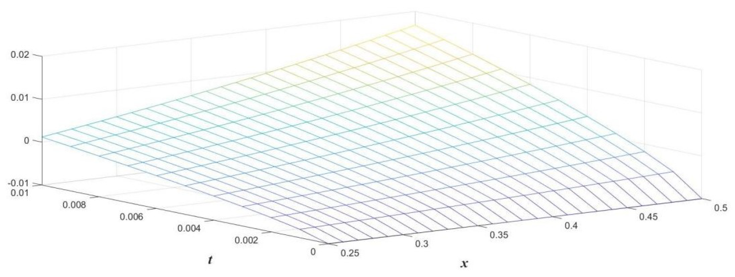
According to Equation (52), if we consider $\alpha =1$, then the third term approximate series solution of Example 2 is expressed as

$$\begin{array}{cc}\hfill u\left(x,t\right)& =x\left(t+0.333t^3\right)-x^2\left(0.5t^2+0.333t^4+0.056t^6\right)\hfill \\ \hfill & +x^3\left(0.5t^2+0.167t^3+0.583t^4+0.167t^5+0278t^6+0.056t^7+0.042t^8+0.006t^9\right)\hfill \\ \hfill & -x^4\left(\begin{array}{c}0.5t^3+0.292t^4+0.75t^5+0.344t^6+0.472t^7+0.194t^8\hfill \\ +0.134t^9+0.038t^{10}+0.014t^{11}+0.003t^{12}\hfill \end{array}\right)\hfill \end{array}$$

(54)

Table 1. Numerical values when $\alpha =0.75,0.9,$ and 1 for Equation (52).

t	x	$\mathit{\alpha }=0.5$	$\mathit{\alpha }=0.75$	$\mathit{\alpha }=1$
		[18] ${\mathit{u}}_{\mathit{LDM}}$	[18] ${\mathit{u}}_{\mathit{LDM}}$	[18] ${\mathit{u}}_{\mathit{LDM}}$
0.2	0.25	0.1128, 0.0912	0.0788, 0.0801	0.0500, 0.0500
0.4	0.5	0.3280, 0.3413	0.2579, 0.2578	0.2000, 0.2001
0.6	1	0.9754, 1.2020	0.7089, 0.7077	0.6016, 0.6015

shows the comparison of values when $\alpha =0.75,0.9$, and 1; $t=0.2,0.4$, and $0.6$; and $x=0.25,0.5,$ and 1 for Equation (52) using the proposed Laplace decomposition method and the Adomian decomposition method [18].

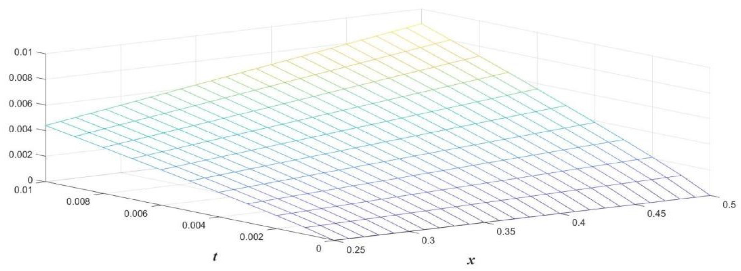
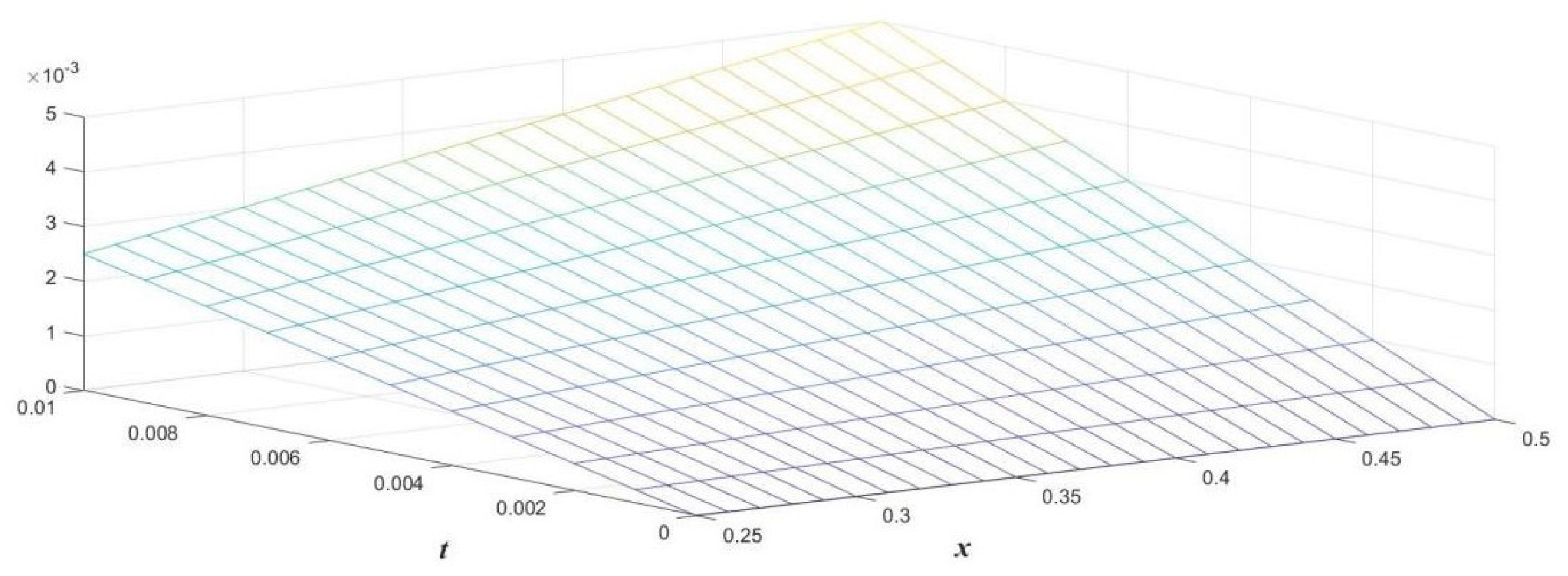
Figure 1, Figure 2 and Figure 3 show the 3D graphical representations of Equation (52) with varying values of $\alpha$.

From Figure 1, Figure 2 and Figure 3 and Table 1, it can be seen that the results are basically consistent with those in references [16,18]. Their error becomes increasingly smaller as the fractional order approaches 1. This is because the conformable fractional derivative is more like the integer derivative than other fractional derivatives [26]. It is worth noting that only three terms of the decomposition series were used to evaluate the approximate solutions for Figure 1, Figure 2 and Figure 3 and Table 1. It can be seen clearly from Equation (52) that the efficiency of the proposed approach can be significantly enhanced by computing the further terms or further components of $u\left(x,t\right)$.

6. Conclusions

In this paper, the general conformable multiple Laplace transform was conducted by using our proposed new scheme. The conformable multiple Laplace transform decomposition method was adopted to solve linear and nonlinear homogeneous or nonhomogeneous partial fractional differential equations. Two numerical examples were provided by using our proposed method. Our results demonstrate the significance of finding novel methods to solve fractional partial differential equations with symmetric variables.

References

1. Khalil, R.; Al Horani, M.; Yousef, A.; Sababheh, M. A new definition of fractional derivative. J. Comput. Appl. Math. 2014, 264, 65–70. [Google Scholar] [CrossRef]
2. Krasnoschok, M.; Pata, V.; Siryk, S.V.; Vasylyeva, N. Equivalent definitions of Caputo derivatives and applications to subdiffusion equations. Dyn. Partial. Differ. Equ. 2020, 17, 383–402. [Google Scholar] [CrossRef]
3. Abdeljawad, T. On conformable fractional calculus. J. Comput. Appl. Math. 2015, 279, 57–66. [Google Scholar] [CrossRef]
4. Bhanotar, S.A.; Kaabar, M.K. Analytical solutions for the nonlinear partial differential equations using the conformable triple Laplace transform decomposition method. Int. J. Differ. Equ. 2021, 2021, 9988160. [Google Scholar] [CrossRef]
5. Gözütok, N.Y.; Gözütok, U. Multivariable conformable fractional calculus. arXiv 2017, arXiv:1701.00616. [Google Scholar]
6. Kaabar, M.K.; Martínez, F.; Gómez-Aguilar, J.F.; Ghanbari, B.; Kaplan, M.; Günerhan, H. New approximate analytical solutions for the nonlinear fractional Schrödinger equation with second-order spatio-temporal dispersion via double Laplace transform method. Math. Methods Appl. Sci. 2021, 44, 11138–11156. [Google Scholar] [CrossRef]
7. Atangana, A.; Oukouomi Noutchie, S.C. On multi-Laplace transform for solving nonlinear partial differential equations with mixed derivatives. Math. Probl. Eng. 2014, 2014, 267843. [Google Scholar] [CrossRef]
8. Zhao, D.; Luo, M. General conformable fractional derivative and its physical interpretation. Calcolo 2017, 54, 903–917. [Google Scholar] [CrossRef]
9. Jarad, F.; Abdeljawad, T. A modifi ed Laplace transform for certain generalized fractional operators. Results Nonlinear Anal. 2018, 1, 88–98. [Google Scholar]
10. Omran, M.; Kiliçman, A. Fractional double Laplace transform and its properties. In Proceedings of the AIP Conference Proceedings, St. Louis, MO, USA, 9–14 July 2017; Volume 1795, p. 020021. [Google Scholar]
11. Ozkan, O.; Kurt, A. Conformable fractional double Laplace transform and its applications to fractional partial integro-differential equations. J. Fract. Calc. Appl. 2020, 11, 70–81. [Google Scholar]
12. Nuruddeen, R.I.; Zaman, F.; Zakariya, Y.F. Analysing the fractional heat diffusion equation solution in comparison with the new fractional derivative by decomposition method. Malaya J. Mat. 2019, 7, 213–222. [Google Scholar] [CrossRef] [PubMed]
13. Bouaouid, M.; Hilal, K.; Melliani, S. Nonlocal telegraph equation in frame of the conformable time-fractional derivative. Adv. Math. Phys. 2019, 2019, 7528937. [Google Scholar] [CrossRef]
14. Özkan, O.; Kurt, A. On conformable double Laplace transform. Opt. Quantum Electron. 2018, 50, 1–9. [Google Scholar] [CrossRef]
15. Khan, A.; Khan, A.; Khan, T.; Zaman, G. Extension of triple Laplace transform for solving fractional differential equations. Discret. Contin. Dyn. Syst. S 2020, 13, 755. [Google Scholar] [CrossRef]
16. Mohamed, M.Z.; Elzaki, T.M.; Algolam, M.S.; Abd Elmohmoud, E.M.; Hamza, A.E. New modified variational iteration Laplace transform method compares Laplace adomian decomposition method for solution time-partial fractional differential equations. J. Appl. Math. 2021, 2021, 6662645. [Google Scholar] [CrossRef]
17. Al-Zhour, Z.; Alrawajeh, F.; Al-Mutairi, N.; Alkhasawneh, R. New results on the conformable fractional Sumudu transform: Theories and applications. Int. J. Anal. Appl. 2019, 17, 1019–1033. [Google Scholar]
18. Odibat, Z.; Momani, S. Numerical methods for nonlinear partial differential equations of fractional order. Appl. Math. Model. 2008, 32, 28–39. [Google Scholar] [CrossRef]
19. Jafari, H.; Khalique, C.M.; Nazari, M. Application of the Laplace decomposition method for solving linear and nonlinear fractional diffusion–wave equations. Appl. Math. Lett. 2011, 24, 1799–1805. [Google Scholar] [CrossRef]
20. Jassim, H.K. The Approximate Solutions of Three-Dimensional Diffusion and Wave Equations within Local Fractional Derivative Operator. In Abstract and Applied Analysis; Hindawi: London, UK, 2016; Volume 2016. [Google Scholar]
21. Baleanu, D.; Jassim, H.K. Exact solution of two-dimensional fractional partial differential equations. Fractal Fract. 2020, 4, 21. [Google Scholar] [CrossRef]
22. Krasnoschok, M.; Pata, V.; Siryk, S.V.; Vasylyeva, N. A subdiffusive Navier–Stokes–Voigt system. Phys. D Nonlinear Phenom. 2020, 409, 132503. [Google Scholar] [CrossRef]
23. Wang, Y.; Zhao, Z.; Li, C.; Chen, Y. Adomian’s method applied to Navier-Stokes equation with a fractional order. In Proceedings of the International Design Engineering Technical Conferences and Computers and Information in Engineering Conference, San Diego, CA, USA, 30 August–2 September 2009; Volume 49019, pp. 1047–1054. [Google Scholar]
24. Yu, Q.; Song, J.; Liu, F.; Anh, V.; Turner, I. An approximate solution for the Rayleigh-Stokes problem for a heated generalized second grade fluid with fractional derivative model using the Adomian decomposition method. J. Algorithms Comput. Technol. 2009, 3, 553–572. [Google Scholar] [CrossRef]
25. Seligman, M.E. Comment and integration. J. Abnorm. Psychol. 1978, 87, 165–179. [Google Scholar] [CrossRef] [PubMed]
26. Tarasov, V.E. No violation of the Leibniz rule. No fractional derivative. Commun. Nonlinear Sci. Numer. Simul. 2013, 18, 2945–2948. [Google Scholar] [CrossRef] [Green Version]
Figure 1. 3D plot of Equation (52) for α = 0.75 , x 0.25 , 0.5 , and t 0 , 0.01 .
Symmetry 15 00389 g001
Figure 2. 3D plot of Equation (52) for α = 0.9 , x 0.25 , 0.5 , and t 0 , 0.01 .
Symmetry 15 00389 g002
Figure 3. 3D plot of Equation (52) for α = 1 , x 0.25 , 0.5 , and t 0 , 0.01 .
Symmetry 15 00389 g003