1. Introduction
In many engineering systems, cylindrical objects are often used, including discs, cylinders, and rods. Therefore, predicting stress and displacement patterns in such geometries is paramount. According to materials science and engineering requirement developments, symmetric axle components have begun to be manufactured from different materials. Due to their superior physical properties, composite materials have gained immense popularity among researchers and technologists. In this regard, there is abundant literature on stress assessments of axially symmetric components composed of different materials that are subjected to diverse loading states.
An essential part of an effective design process is a comprehensive understanding of the patterns of thermal stresses in the rotating discs. Rotating materials are also used in many industrial applications, such as flywheel rotors, deflation installation, engineering equipment, high-speed gear motors, turbines, computer hard disks, compressors, etc. The use of elastic waves traveling through inertial space is somewhat diverse. It specifically serves as the basis for designing sound wave solid-state gyroscopes, which have recently received much attention. This can be explained using different gyroscopes in moving objects’ guidance and navigation systems. Gyroscopes based on sound waves offer higher resistance to vibration and shock, are less expensive, and require less complex manufacturing processes. In the existence of collective forces of the Coriolis type, these waves are characterized by motion equations. Numerical techniques can be utilized to solve these equations. However, in this case, the accuracy of the wave process simulation deteriorates steadily over time.
Temperature influences the thermomechanical characteristics of substances. A materials’ structural components are often subjected to high-temperature changes, and their physical properties cannot be considered stable, so they are used for a variety of engineering purposes. Thus, while analyzing the thermal stress of these components, the temperature dependence of the physical properties must be considered. In recent years, the significance of isotropic thermal stress difficulties for contemporary systems, such as nuclear reactors, has increased. This is because there are more kinds of engineering designs, and more work is conducted in places where it is very hot.
The concept of thermoelasticity explains the effect that thermomechanical disturbances have on substances that are either elastic or viscous. The theory of heat transfer is based on two equations. The first equation is about how heat moves and is transferred, and the second equation is about how things move. There are two disadvantages to this idea in the conventional approach. First, this derivation of heat transmission does not contain any elastic components. The second issue is that, according to the parabolic heat transfer equation, the temperature may continue to rise at a steady pace that cannot be slowed down. This is an intractable problem. Experiments have shown that this is the case.
In traditional thermoelasticity, stresses, tensions, and deformations resulting from observable thermal stress were anticipated. The old coupled thermoelasticity notion held that heat signals would propagate at an unlimited pace, prompting the development of generalized thermoelastic models. The concept of thermoelasticity can be applied to a variety of physical processes. It is a modification of the traditional ideas of elasticity and thermal conductivity, and today it is a fully formed scientific topic. Based on this concept, there were some problems related to the propagation of thermoelastic waves, which were addressed and solved. Biot [
1] developed a theory that was later dubbed conventional thermoelasticity based on the notions of irreversible thermodynamic systems. In the case of classical coupled thermoelasticity, the distribution and amplitude of thermal stresses and temperature change are immediately affected by the thermal shock effect throughout the solution domain. Thus, thermoelastic turbulence can theoretically propagate at an unlimited rate. On the basis of this analysis, improved thermoelastic models that incorporate finite wave propagation velocity are presented. Improved thermoelastic models use either an improved Fourier law of heat transfer or a revised entropy formulation and constitutive law.
Cattaneo [
2] modified Fourier’s law of heat transfer by introducing a single relaxation time. Then, the vibration-type equation was developed rather than the conventional Fourier law. According to Lord and Shulman [
3], the first alteration was made. Since the heat conduction equation associated with this model is of the deterministic-type, the problem of unlimited diffusion speed was solved. The rate-dependent thermoelastic concept, also known as the two-time relaxation thermoelastic framework, is the second application of the thermocouple idea. The authors of this second idea are Green and Lindsay [
4]. As a result of the existence of these two parameters, which play the role of “relaxation times” and are an integral element of this system, the equations for heat transfer and motion need to be modified in this particular instance.
Later, on the basis of the inequalities of the entropy balance, Green and Naghdi [
5,
6,
7] proposed three other inventive formulations of thermoelasticity. They use the GN-I, GN-II, and GN-III types of thermoelasticity. Type I might become the standard heat equation in a system of linear equations, whereas the type II and type III versions forecast the restricted rate of thermal waves following linearization. There have been recent efforts by Abouelregal [
8,
9,
10,
11,
12,
13,
14] to use higher-order time derivatives to modify the traditional Fourier formula.
When the traditional Fourier law is applied to the process of wave propagation, a disagreement may be shown (for example, in [
2,
3,
4]). This inconsistency is what causes the issue of unlimited signal velocity. While constructing the sound wave equations as well as the heat transfer equation, many different constitutive relationships for heat transfer rate are taken into consideration as a consequence. A novel thermoelastic heat transfer framework is being developed by Quintanilla [
15] using the Moore–Gibson–Thompson (MGT) equation. A brand new and better heat equation that incorporates a relaxation parameter has been proposed by Quintanilla [
16] for the Green–Naghdi concept of type III. The Westervelt and Kuznetsov equation is an example of a traditional second-order in time heavily damped theory of linear acoustics. There has been a lot of research conducted on this topic since it has a wide variety of applications, such as high-intensity ultrasound in the fields of health and extracorporeal shock wave therapy, light treatment, ultrasonic washing, and many more applications. There has been a proliferation of research on this topic ever since the MGT model came into existence [
16,
17,
18,
19,
20,
21]. In recent years, there has been a significant application of the literature study of thermomechanical and structural interactions across several systems [
22,
23,
24,
25,
26,
27].
Since the eighteenth century, scientists have been searching for the phenomena of thermomechanical and electromagnetic behaviors of solids. In the middle of the 20th century, hydrophones were the first to use materials with piezoelectric properties. Before the 1960s, researchers looked at something called the thermomagnetic flexibility theory [
28]. This significant phenomenon may be utilized in a broad variety of contexts, such as in the discipline of geophysics, where it is used to investigate how the Earth’s magnetic field influences seismic waves and how it attenuates sound waves while they are contained within the magnetic field. In addition, devices based on nuclear fission, the development of a very sensitive magnetometer, advances in electrical power engineering and optics, and other fields may all benefit from research into interactions between thermomechanical and electromagnetic materials [
29].
Over the past two decades, electromagnetic composite structures have been brought to light. Unlike their homogeneous constituent materials, these compounds can display field coupling. The use of so-called “smart” materials and combinations may be useful for developing many components, including ultrasound imaging technologies, sensor systems, electrical control devices, transducers, etc. These materials are utilized rather regularly in a wide variety of different applications [
30]. Because of their versatility in converting various kinds of energy, these materials have found use in a variety of high-tech applications, including lasers, supersonic devices, microwave ovens, and infrared applications (between mechanical and electromagnetic energies). On the other hand, ferromagnetic materials have impacts that are analogous to those of mechanical forces: electromagnetic fields [
31].
On the basis of considering the thermal motion, the current work introduces a new explanation of extended thermoelasticity. Additionally, this article addresses the problem of thermoelastic–magnetic interactions occurring within a transverse isotropic circular cylinder by using the concept of a novel theoretical formula for modified thermal conductivity (MGTTE), which incorporates the MGT equation. In the presence of a magnetic field and according to the modified Ohm’s law, the equations are obtained from the previously made framework that regulates the behavior of generalized thermoelastic. Theoretically, thermoelastic waves will move through heat conduction at a finite speed. This is predicted by the theory based on photothermal motion. Therefore, generalized thermoelastic theories are more appropriate than classical thermoelastic concepts when dealing with experimental and theoretical systems involving very short periods and high temperatures. Examples of these types of problems include those that actually occur in lasers, power generation, nuclear reactors, and other similar settings.
For the purpose of studying and clarifying the problem posed, it was taken into consideration that the inner edge of the hollow cylinder is devoid of traction force and is subject to a time-dependent thermal shock. On the other hand, it was assumed that the border on the outer side of the cylinder is free of traction but acts as a heat insulator. The problem was solved by applying the Laplace transform methodology to convert the system of equations into a normal system. Then, the reflections of the Laplace transforms were calculated using one of the numerical methods. The results of the numerical simulation of the material properties that are the focus of the research, such as temperature, thermal stresses, and deformations, were compiled and compared with the corresponding previous results through the use of graphs and tables. Computation was performed to evaluate how the non-Fourier model influences the transmission of heat and thermoelastic vibrations under thermal relaxation and the existence of an applied magnetic field. When the current study was compared to earlier investigations, the numerical results were determined to be broadly comparable.
The general structure of the paper is divided into the following sections: Moore–Gibson–Thompson’s equations for basic thermoelasticity are presented in
Section 2. While the limit and starting conditions are provided in
Section 4, and the problem statement, which includes the transverse isotropic cyclic cylinder, is covered in
Section 3. The Laplace transform technique is used in
Section 5 to obtain an answer to the question in the transformed domain.
Section 6 reflects the numerical findings of the Laplace transforms. The numerical results of the research areas in
Section 7 are compared in three separate scenarios, and the main results are presented in
Section 8.
2. Moore–Gibson–Thompson Thermoelasticity Fundamental Equations
The following are the constitutive, strain–displacement, and motion equations for a homogeneous transversely isotropic material [
24,
25,
26]:
When the medium rotates symmetrically with rotation speed
, where
is an input vector indicating the direction of the rotation axis, the equation of motion in the rotating reference frame has two additional components [
23]. When the only cause of gravitational acceleration is the time-varying motion
, and also assuming that the Coriolis acceleration
is twice the centripetal acceleration, the equation of motion in a rotating medium can be stated as [
23]:
After Equations (2) and (3) are entered into Equation (4), the final equation of motion will take the following form:
By making use of the GN-III model, we can describe Fourier’s law by characterizing it as [
7]:
As can be shown, type II (GN-II) may be attained when ; however, kind I (GN-I) can be returned when .
The formula for calculating the energy balance is stated as [
3,
4]:
The problem with the modified version of Fourier’s law (7) is the same as the problem with the normal Fourier model regarding predicting the speed at which heat transfer waves propagate. The law of causation is ignored in this approach. As a result, a relaxation factor was added to this guideline, which has also undergone a major update [
15]. Quintanilla [
16] took the Green–Naghdi type III model and added the relaxation coefficient to work out the proposed heat equation. The mathematical model for the new heat transfer is, thus, written as [
15,
16]:
The MGT equation for isotropic solids was used to develop a unique linear version of the heat transport equation. Equations (8) and (9) are combined to obtain this equation. This equation is referred to as MGTTE and takes the following form:
It was assumed that the primary magnetic field,
, propagates in the surrounding vacant space of the cylinder. This field creates generated electric and magnetic fields (
and
) to satisfy slow-moving matter and Maxwell’s magnetic formulas. Maxwell’s equations listed below regulate the electromagnetic field in the absence of the influence of displacement current and charge density [
32]:
It is possible to represent the Maxwell stress tensor in the following manner:
Generalized Ohm’s law may be expressed as follows when the temperature gradient effect is ignored:
Only a substance’s electrical conductivity can be used to determine how well it can carry an electric current. Many materials show a wide range of electrical conductivity values, depending on how well electricity can flow through them. Many scientists assume that the substance is totally conductive (has zero resistance) and that electrical conductivity will, thus, go on infinity (i.e., ). Physically, however, this is unacceptable because all conductive materials have a finite electrical conductivity. Although there are no perfect electrical conductors in reality, the idea can be used when the electrical resistance is very small compared to other elements.
3. Problem Statement
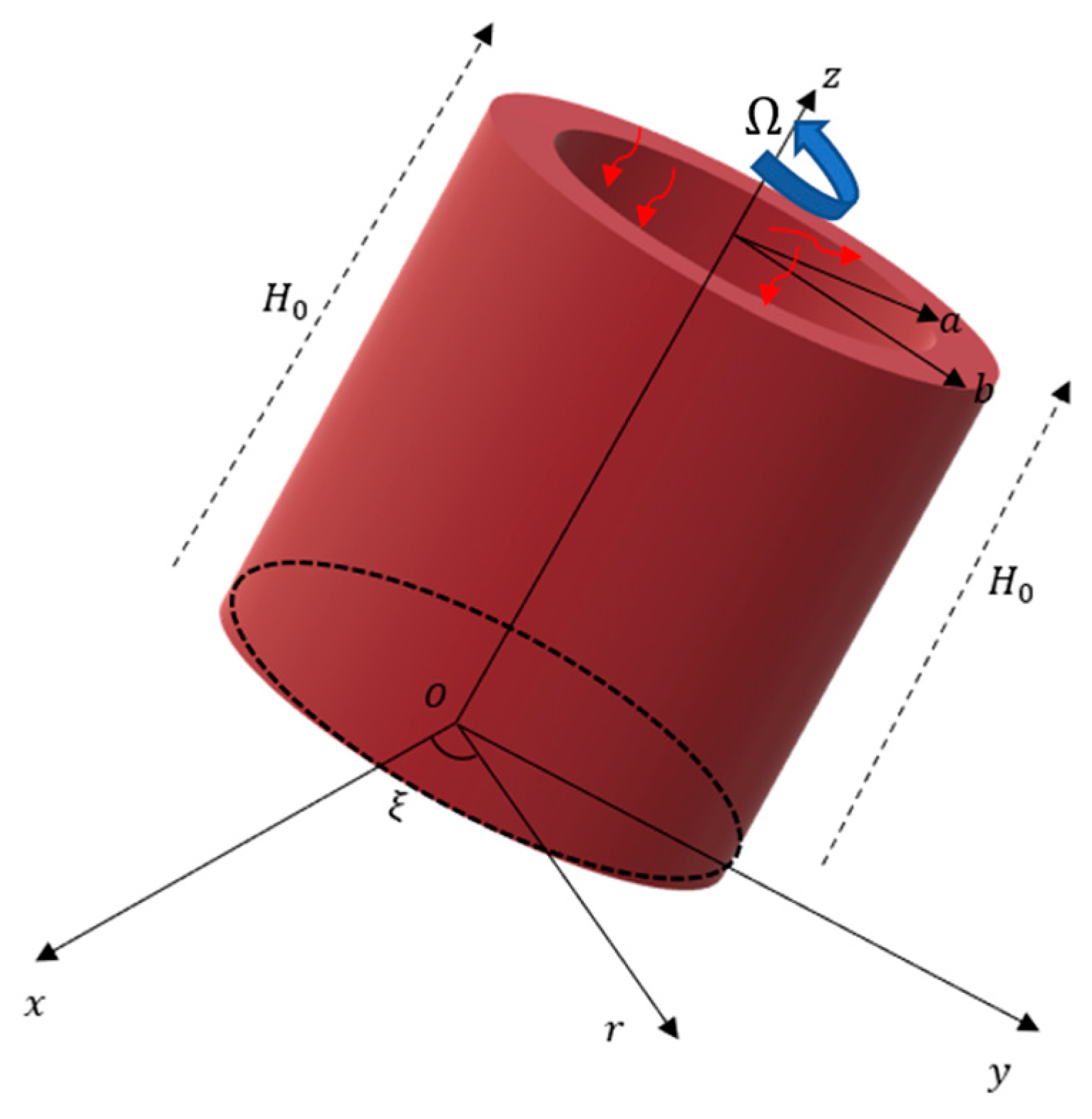
In this article, it will be assumed that the problem under study is an infinite thermoelastic hollow cylinder consisting of an isotropic, homogeneous material with finite conductivity (see
Figure 1). At a constant temperature of
, the body begins in an undisturbed state with no deformations or stresses. We will assume that the inner radius of this cylinder is
, and its outer radius is
. The inner and outer surfaces are free of traction and constrained by certain thermal boundary conditions. A time-dependent symmetrical thermal shock will be delivered to its inner surface, while the outer surface is thermally insulated. Due to the characteristics of the problem at hand, the cylindrical polar coordinates
will be taken into account in the study so that the
z-axis corresponds to the cylinder axis. Given the cylindrical symmetry of the problem, there will only be two variables to consider: the variable representing the diagonal distance,
r, and the variable representing the passage of time,
.
As a direct result of this assumption, the displacement vector consists of the following components:
Then, the corresponding strain components will be derived as:
Consequently, the cubic dilatation,
, can be expressed as:
The following can be inferred about the parts that make up the mechanical stress tensor,
:
where
,
, and
represent the normal thermal stresses.
It will be taken into account that the rotation will occur around the
z-axis so that the angular velocity vector is
. Thus, the motion Equation (5) under the influence of the Lorentz force (
) and the force that is exerted on the body as a direct consequence of its rotation
can be reformulated as follows:
The following relationship determines
, which stands for the Lorentz force brought on by the existence of the magnetic field:
Here, both the components of the externally supplied starting magnetic field (
) and the components of the internally generated magnetic field are taken into consideration
:
These equations unequivocally demonstrate that only the
-direction contains the non-vanishing components of the vectors
and
, i.e.,:
A linearization of Ohm’s law (13) yields:
The following two equations can be obtained in our case from Equation (11):
In the space outside the cylinder, we can derive the two equations shown below:
where
and
stand for, respectively, the intensity of the electric field and the magnetic field induced, both in the
-direction, in the open space around the cylinder.
When the variable
is taken out of Equations (22) and (23), we obtain:
Again, when we remove
from Equations (23) and (25), we obtain:
where
is the Laplace operator.
The Maxwell stress tensor
in our situation has a radial component that is specified by:
The body force, also known as the Lorentz force, may be described in the radial direction with the help of the following equation:
The motion equation has the form when Equations (17), (18), and (28), respectively, are employed:
By using the div operator on both sides, we can obtain the following equation, where
for a transversely isotropic body:
The modified MGT heat conduction equation (MGTTE) (10) can also be expressed as follows:
The system equations will be made simpler by using the non-dimensional variables listed below:
Having done away with the dashes for simplicity, (24)–(26), (29), and (30) become:
where:
The parameter indicates light speed, while the parameter indicates magnetic viscosity. The generalized thermoelasticity equations are simplified in the following formulations by leaving out magneto-electric effects if , , and are all equal to zero.
Additionally, this equation can be used to express the non-dimensional constitutive equations:
where:
5. Problem-Solving Approach
The Laplace transform method has major advantages in many applications of practical mathematics. It can be made from various objects, including functions, measurements, and distributions. Equations (33) through (40) are transformed, and the following equations are acquired by using the Laplace transform under the initial conditions stated in Equation (42):
where:
After eliminating
and
from Equations (53)–(55),
solves the following sixth-order differential equation:
where:
The factorization of Equation (38) yields:
where
,
, and
denote the solutions to the characteristic polynomial:
The following is a legitimate illustration of Bessel’s Equation (59) solution, which is written as:
where the parameters
and
, with
are some parameters that only rely on
, and
and
are zero-order-modified Bessel functions of types 1 and 2, respectively.
The following solutions can be expressed similarly:
Equations (52) and (53) yield:
The following is the outcome of substituting Equation (61) into Equation (16), which is integrated with respect to
:
The well-known relations of the Bessel function, which are as follows, are used to determine the displacement
:
Equation (49), when the values from Equations (63) and (65) are entered, yields:
In order to obtain the induced fields in free space,
and
, one must remove
from Equation (50), which results in:
The solution of Equation (51) is given by:
where
and
denote the integration parameters.
By utilizing connection (66) and adding Equation (67) into Equation (50), we obtain:
Additionally, we can arrive at:
When Equations (62), (65), and (73) are replaced with (51), the components of the stress tensor are
After substituting Equation (65) into (52), we obtain:
The boundary conditions (43)–(48) are changed into the following after using the Laplace transforms:
Substituting the solution functions into Equations (62), (63), (67), (69)–(72), and (74) in the above boundary conditions gives a linear system of equations in the unknown parameters, , and , . The values of these constants can be set by resolving this system. As a result, the Laplace transform field achieves an integrated solution to the issue. The next stage is to identify the inverse transformations of the examined domains of the system and their transformation into the space–time domain.
7. Discussion and Graphical Representation
For the purposes of computation, a physical substance was proposed with equidistant physical constants. A numerical example will be considered, and numerical solutions will be provided to illustrate the analytical technique presented earlier in this article and to compare the theoretical results. Mathematica computer programs were used to perform the numerical calculations. The following is a listing of the physical parameters for magnesium (Mg) [
28]:
In the computations, we assume that the inner radius of the cavity is equal to one () and that the outside radius is equivalent to two () concerning the center of the hole. We also assume that one value of time () is used unless anything other is given.
In three separate scenarios, we perform calculations utilizing the aforementioned physical parameters. In the first situation, we will look at how the non-dimensional physical field variables respond to the change in the applied magnetic field. At the same time, the time, relaxation time, and rotation remain fixed. The second aim of the discussion is to investigate how non-dimensional temperature (denoted by ), radial displacement (indicated by ), and thermal stresses (characterized by and ), as well as other electromagnetic fields, change (, , and ) in the case of applying a variety of thermosetting models. The third case study examines how the investigated field variables vary with the variation in the angular velocity of rotation while keeping the values of all other effective parameters constant. The numerical results obtained from several research areas will be presented in tables and figures to facilitate a comparison and discussion of the issue at hand.
7.1. The Influence of Magnetic Field
This section examines thermoelasticity waves in a hollow elastic cylinder with a stress-free boundary and electrical conductivity. A magnetic field is positioned around the inside surface of the cylinder. The first case is an investigation of non-dimensional studied fields using the suggested generalized MGT thermoelastic model (MGTTE) in the existence
and absence (
H0 = 0).
Figure 2,
Figure 3,
Figure 4 and
Figure 5 depict alterations to the spatial coordinates.
It is clear from looking at the graphs that the variance behavior of the fields changes over a period of time. The results evidently demonstrate that the applied magnetic field considerably impacts each investigated field. The phenomena of restricted propagation velocity are another aspect that can be seen in all graphics. On the other hand, the speed of propagation of linked and uncoupled conventional thermoelasticity theories is unlimited. Anywhere in the medium away from heat sources and thermal disturbances, all associated functions have finite possible values.
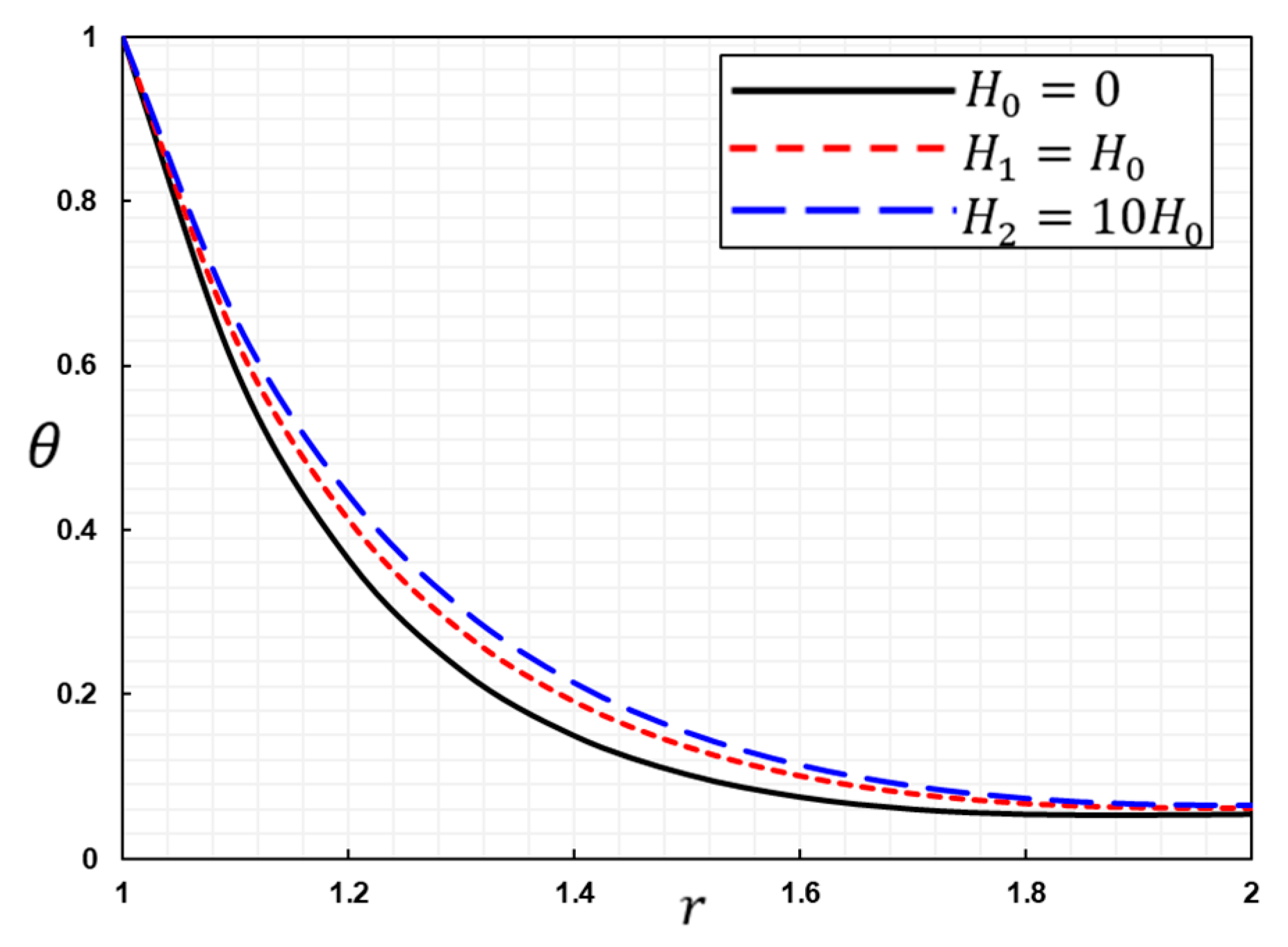
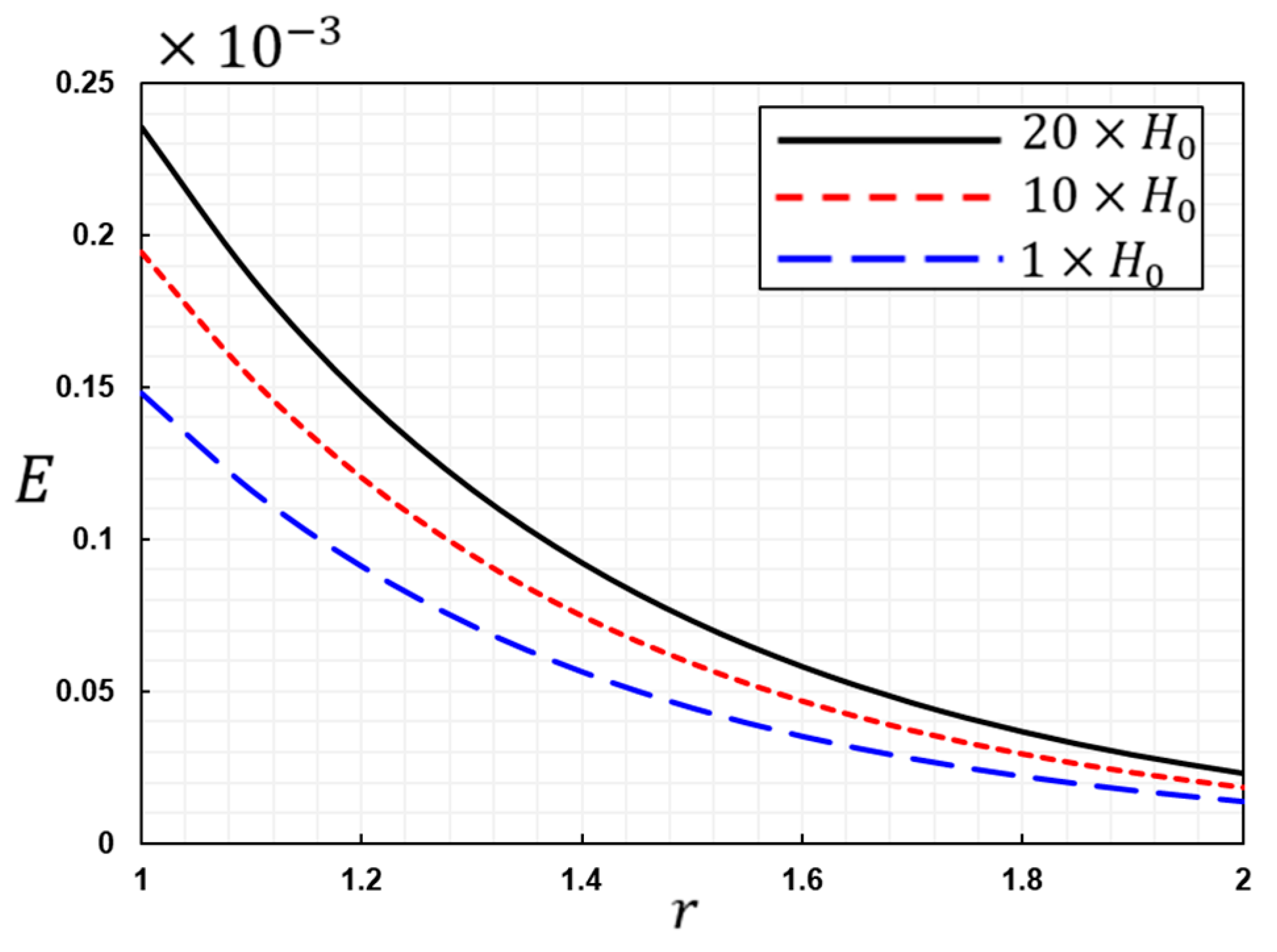
Figure 2 depicts the fluctuation in temperature
throughout the radial distance
. As seen in
Figure 2, the initial magnitudes of the temperature variations are larger and decrease with time to guarantee that they match the boundary criteria. Additionally, for all
values, it decreases rapidly as the distance from the center grows. The heat wave front advances at a constant rate throughout time. At a particular time, the temperature is non-zero in just a limited spatial field, as indicated by the figure. There is evidence of thermal oscillation in the area that is immediately next to the heat shock, but the level of turbulence decreases as one moves further away from this location. In several areas, the non-zero area fluctuates constantly and continuously. Although the magnetic field has little impact on the temperature change
, it contributes to a rise in the quantity of temperature variation.
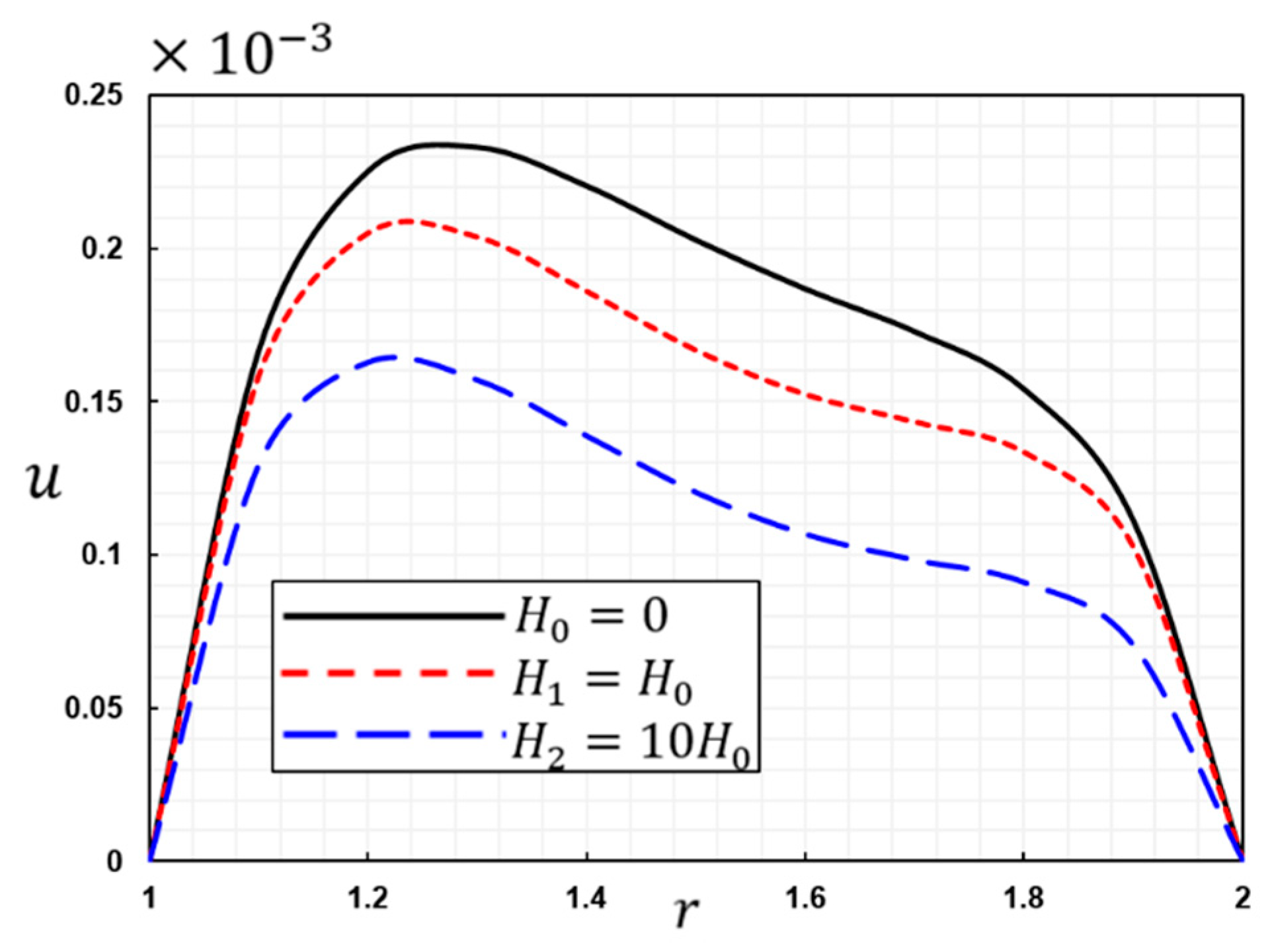
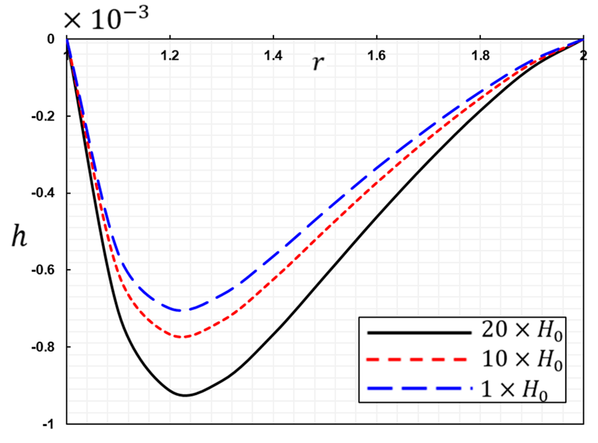
Figure 3 depicts the relationship between the radial displacement
and the radial distance
for various magnetic field strengths. As shown in
Figure 3, the displacement variations at the side walls of the hollow cylinder with
and
conform to the boundary conditions since they always begin and terminate at zero. This distortion is due to a dynamic occurrence. When the values of the magnetic field
grow, the magnitudes of the displacement
decrease.
Figure 3 demonstrates that the wave action restricts the temperature to the non-zero area of the radial displacement at a particular instant. There seems to be a rate restriction for heat transmission to the deeper layers of the medium over time. Thermal vibration and radial displacement area both increase proportionally to the examined moment.
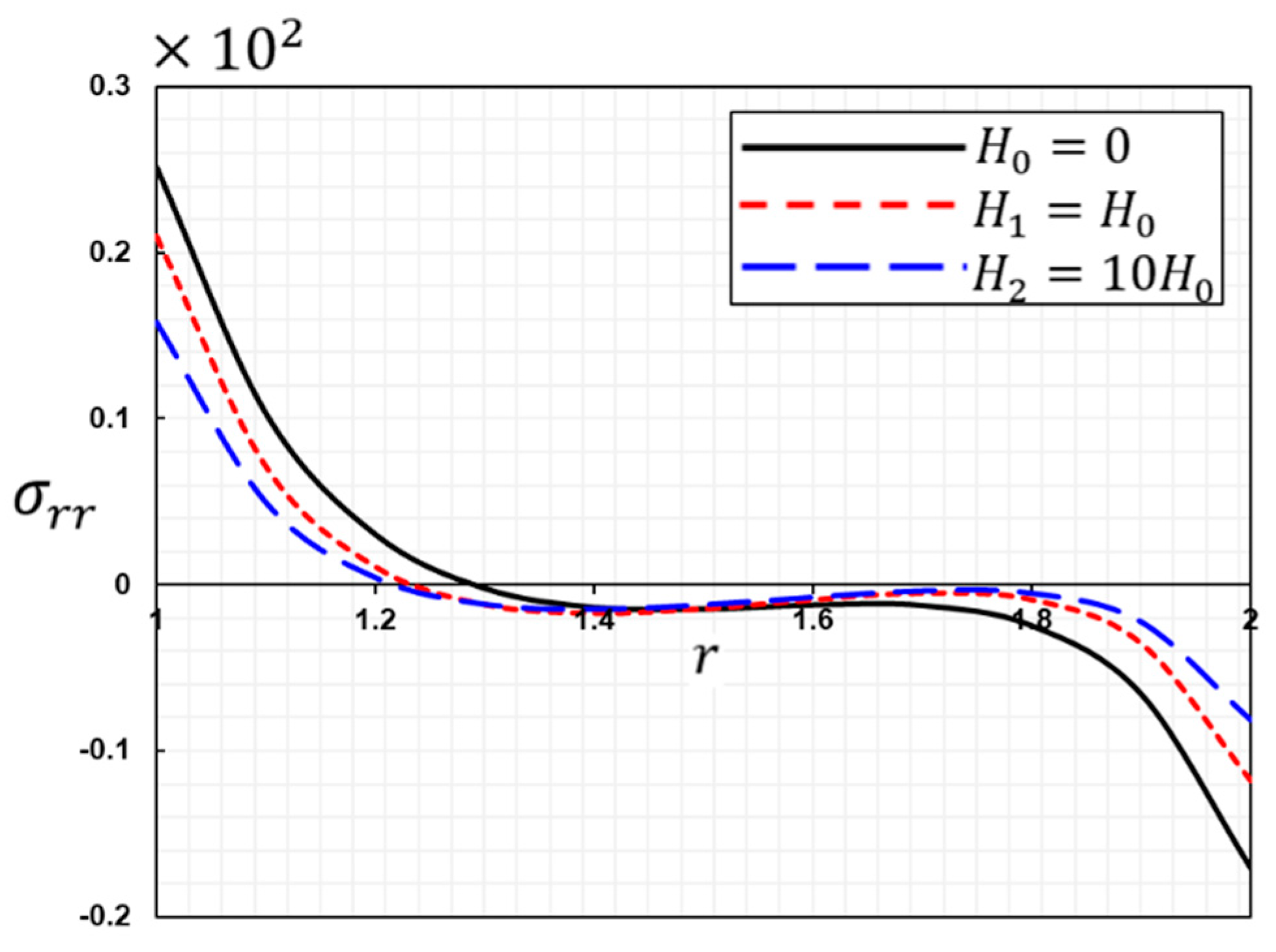
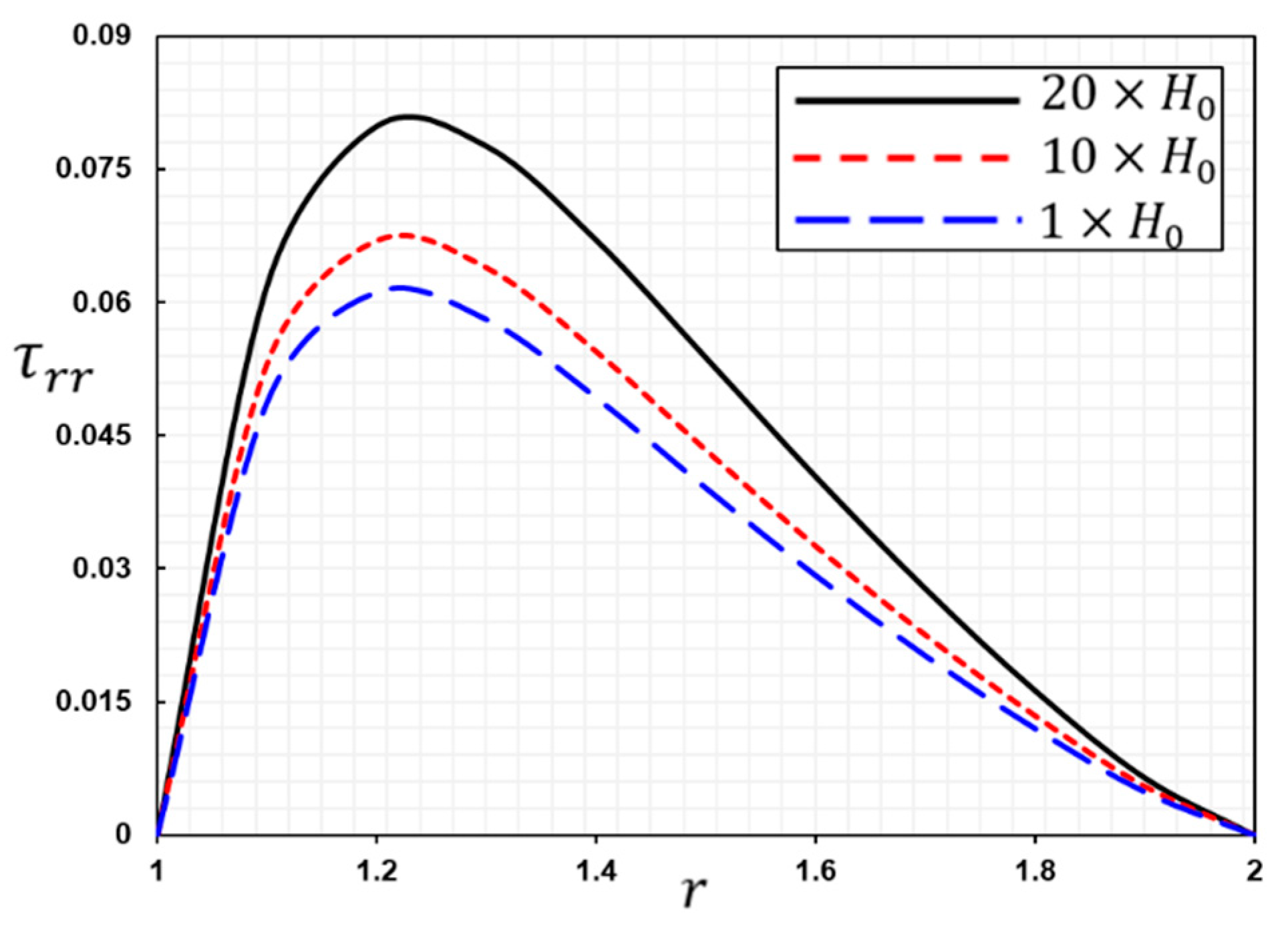
Figure 4 illustrates the relationship between radial tension
and radial distance r for each sample. Observe that the radial stress
increases fast to zero values after immediately reducing to a minimal value. It is clear from the graph that the heat stress starts with its largest positive value at the inner boundary and then decreases after that until it reaches its lowest negative value at the outer boundary of the medium. The values of the primary magnetic field
increase the pressure
, which is another finding from the graph. The material on the inside boundary of the solid is affected by thermal stress. This change corresponds to the radial expansion deformation of the medium, which can be seen in
Figure 4. It can also be seen that with time, the tensile stress region is stretching, while the compressive stress region is contracting. This phenomenon is consistent with the dynamic stretching effect that has been discussed in several previous studies.
Figure 4 provides further evidence that the non-zero stress region is constrained at a point relatively close to the temperature shock effect region. It also demonstrates how temperature waves affect the stress current oscillation.
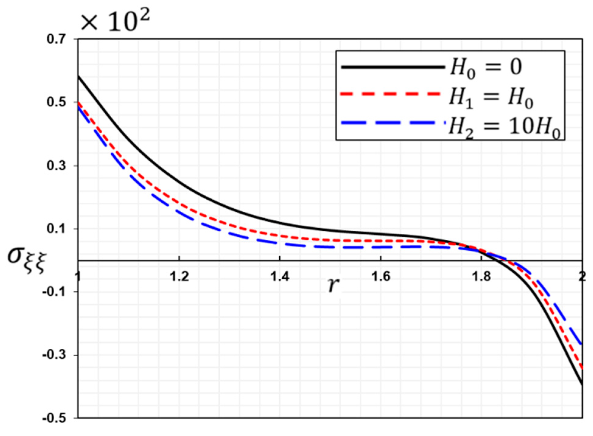
Figure 5 shows the response of the stress distribution,
, with the change in distance r in the existence and absence of the influence of the initial magnetic field,
. The transverse isotropic material shows circumferential compressive stress, as shown in the schematic diagram. It is also evident from the picture that the thermal stress,
, acts similarly to the radial stress,
, except that the ring stress begins with larger positive values. It can also be seen from
Figure 4 and
Figure 5 that stress occurs in one area of the cylinder while stress occurs in another. The area near the inner surface of the cylinder is subjected to increased tensile stress as it diminishes on the other side. The amount of stress increases with the height of the magnetic field surrounding the cylinder, as shown in
Figure 4. This indicates that in addition to the thermal shock effect, the effect of the parameter
extends to the hollow cylinder.
Figure 6,
Figure 7 and
Figure 8 demonstrate the distributions of induced magnetic field
, induced electric field
, and the Maxwell stress
in the hollow cylinder with three different values of the axial magnetic field (
, 10
, and
). The accompanying thermoelastic–electromagnetic interactions are conveniently shown in
Figure 6 and
Figure 7. The electromagnetic material, which is originally contained within a magnetic field, undergoes distortion due to thermal shock. As a result, the magnetic field strength across the cross-section of the cylinder changes. As a direct consequence of this, the medium possesses both an induced magnetic field and an induced electric field. The magnetic and electric fields that are produced by the heat wave will undergo transformations as it travels further inside the cylinder. This is another piece of evidence that temperature changes may cause wave responses.
This study shows that the axial magnetic field coefficient
of variation has a considerable impact on the conduct of all induced fields, including electric and magnetic ones, highlighting the significance of taking into account the influence of
.
Figure 6,
Figure 7 and
Figure 8 show that when
is equal to
and
, the numerical values of all of the field variables are greater than they are when
is equal to
. The many engineering uses of this type of material and piezo plates include applications such as turbine membranes, marine construction, and nuclear reactors. It also contains other uses, such as building ships and cars, spacecraft, and others.
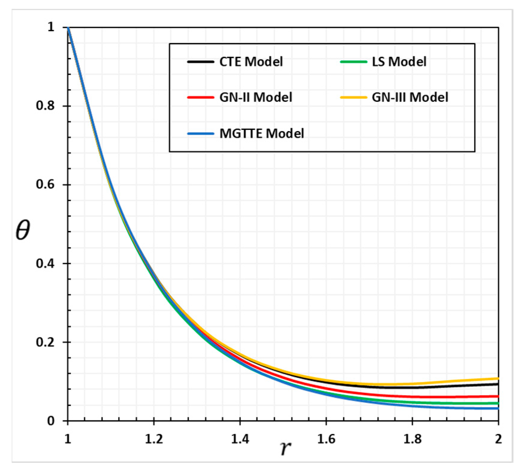
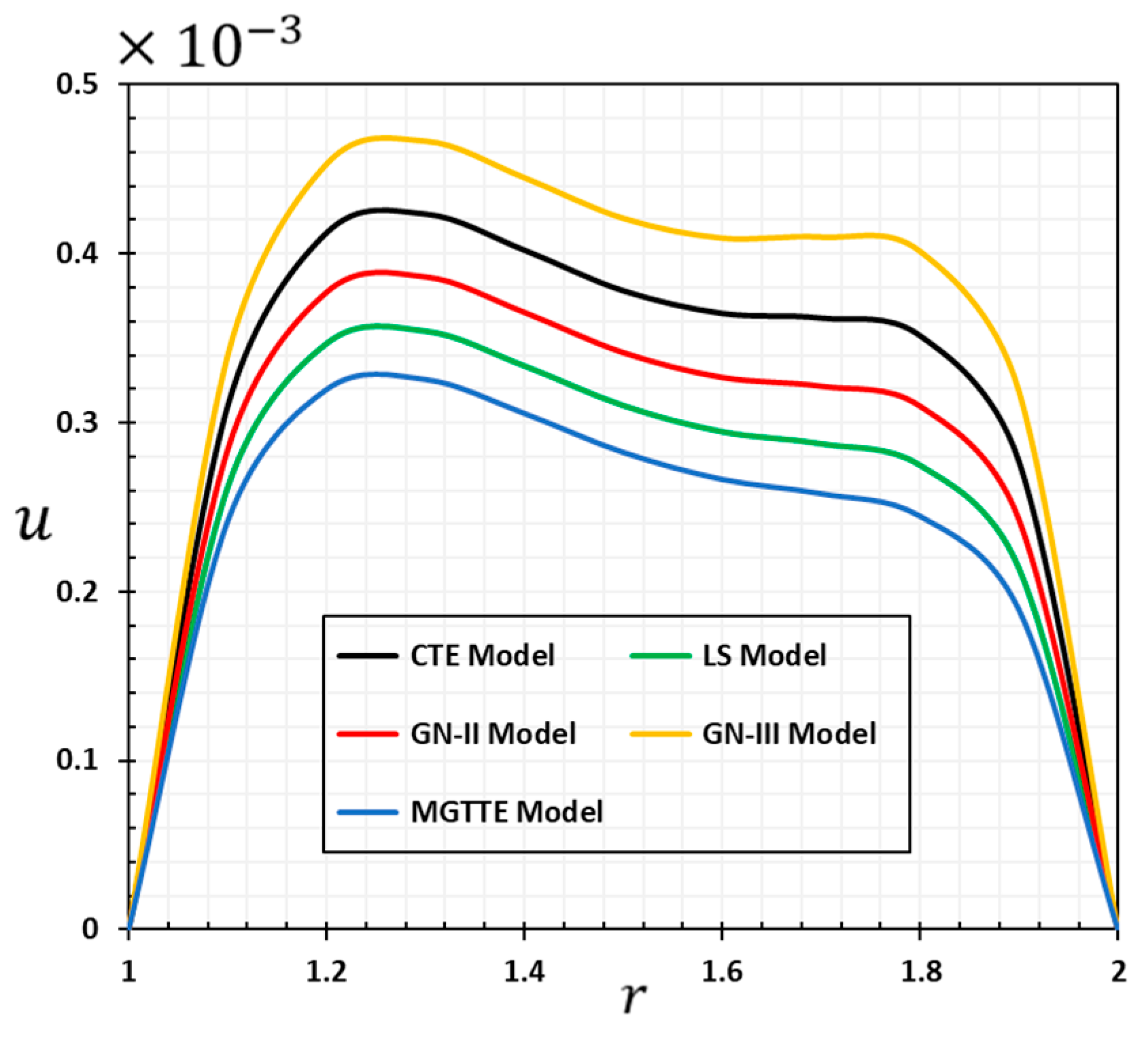
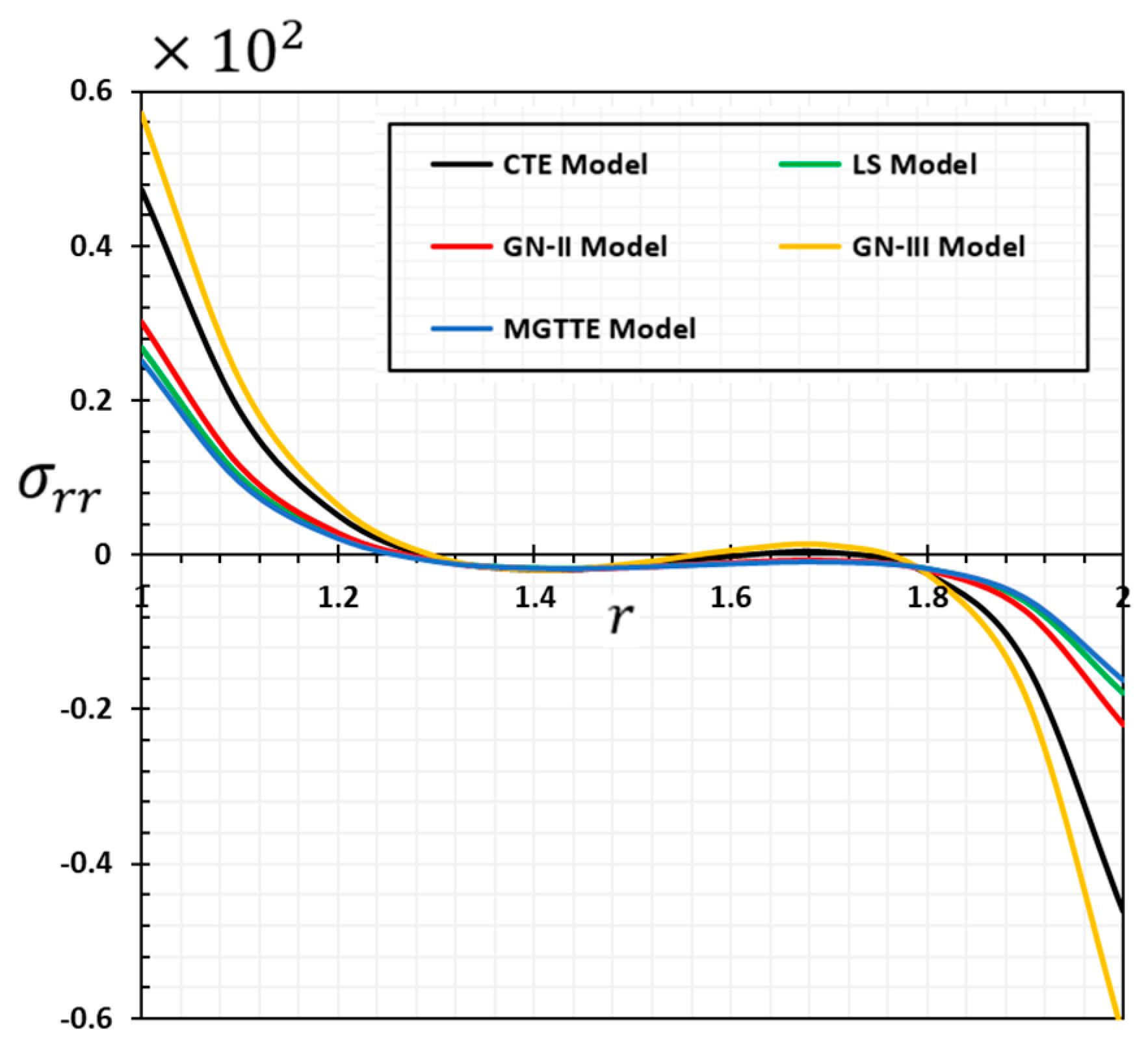
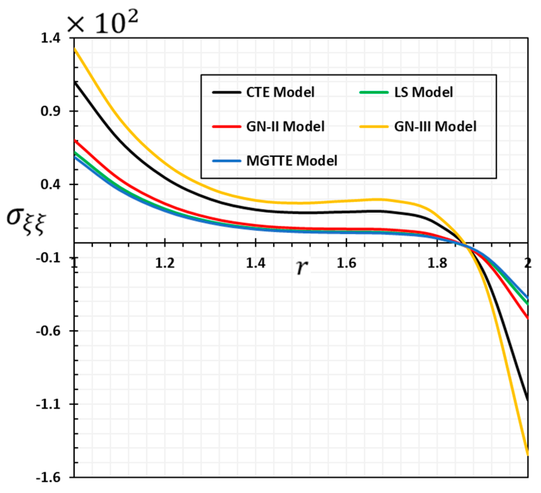
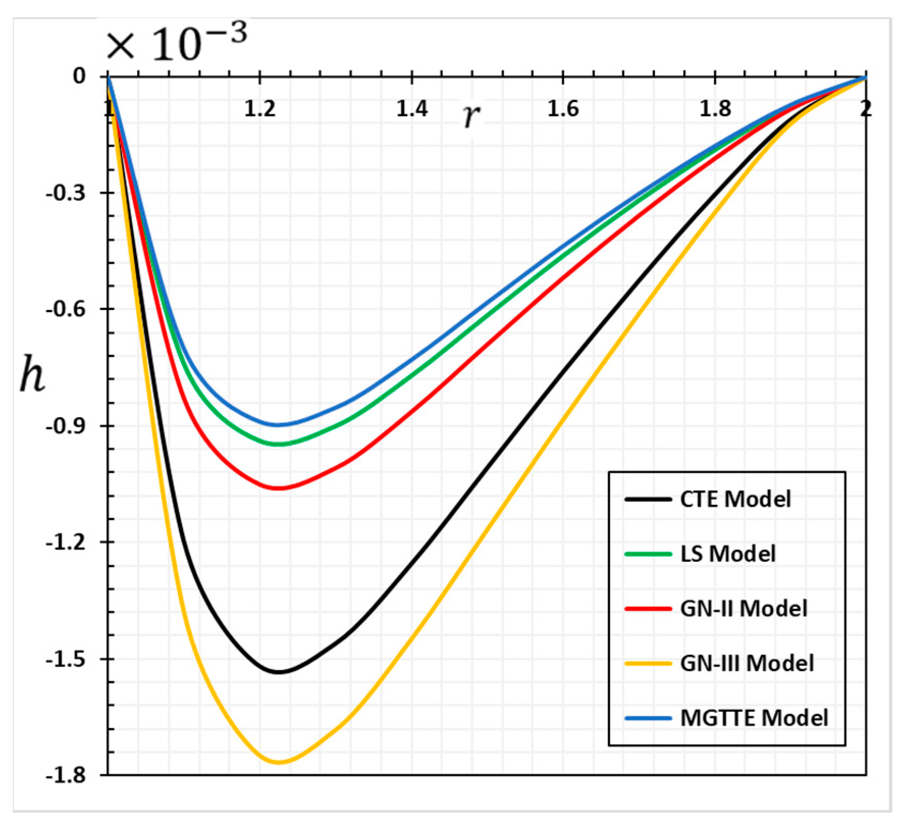
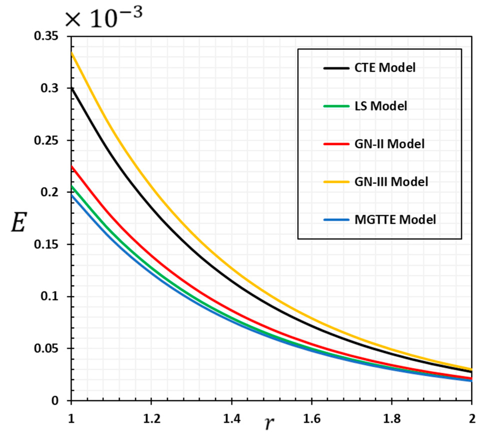
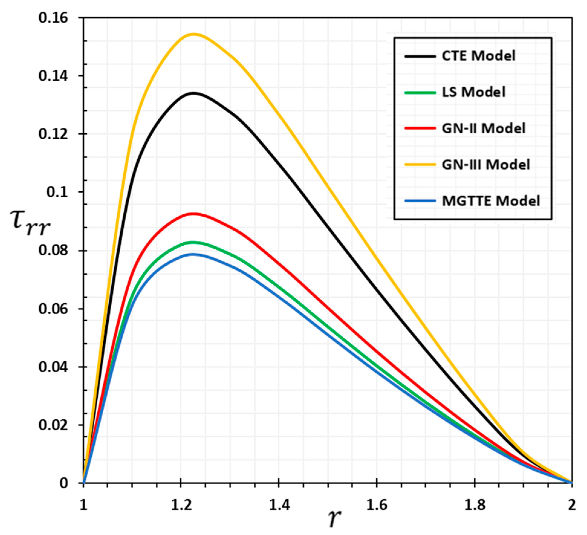
7.2. Thermoelastic Models
The behavior of thermal, mechanical, and electromagnetic field variables in relation to radial distance
will be investigated in the context of various thermoelastic theories in the second scenario of this debate. Axial magnetic field
and
time will stay unchanged in this scenario. To show the distinctions between the various theories of thermoelasticity and how they relate to one another,
Figure 9,
Figure 10,
Figure 11,
Figure 12,
Figure 13,
Figure 14 and
Figure 15 each show a distinct variation in the physical fields. Numerous earlier models in general thermoelastic theory will be shown as special instances in the model described in this article.
When , one can derive the coupled dynamical thermoelasticity theory (CTE), whereas results in Lord Shulman’s model (LS). When the term that contains the parameter is equal to zero and there is no thermal relaxation factor, the second sort of Green–Naghdi theorems, which are denoted by the notation GN-II, can also be produced. On the other hand, if one disregards the thermal relaxation period, it is possible to produce the third kind, denoted by the GN-III. When thermal relaxation , and parameters are present, the MGT extended heat conduction theory is valid (MGTTE).
Table 1,
Table 2,
Table 3,
Table 4,
Table 5,
Table 6 and
Table 7 and
Figure 9,
Figure 10,
Figure 11,
Figure 12,
Figure 13,
Figure 14 and
Figure 15 in this subsection’s results presentation, which aim to make it easier to compare various thermoelastic models, provide the findings. Future scientists can use the tables in this page to compare their findings. It is clear from the tables and figures that the temperature parameters have a significant impact on the distribution of the investigated field values,
and
. It is also obvious that the different thermal models have a different impact on the values of the fields. When the boundary conditions imposed by the proposed problem are present, the behavior near the inner cylinder surface is very comparable for both the coupled (CTE) and generalized (LS, GNII, GNIII, and MGTTE) thermoelastic models. The results are comparable as the distance increases and agree with generalized thermoelasticity theories.
According to the coupled theoretical model, in contrast to the extended thermoelastic theories, which suggest that heat waves travel at a finite pace, heat waves move at an infinite speed. Furthermore, the numerical analysis results make it clear that the heat wave moves from the inside to the outside of the cylinder because the thermal shock is only given to the inside edge of the solid.
Table 1,
Table 2,
Table 3 and
Table 4 and
Figure 1,
Figure 2 and
Figure 3 illustrate the discrepancy between the GN-III and MGTE model predictions (9–15). The results show that the statistical results and curve fields for the GN-III version are larger than those for the MGTE model. It is also pointed out that both the LS and MGTE models exhibit the same numerical findings and behaviors. This is due to the presence of a thermal relaxation period. The results of the GN-III heat conduction model by Green and Naghdi demonstrate a clear departure from the reduced energy dissipation type II heat transfer ideas (GN-II). Significant temperature values and distribution differences exist between the GN-II model and the other models.
These examples unequivocally demonstrate that, in the expanded Moore–Gibson–Thompson thermoelasticity theory, the wave propagation rates are constrained (MGTTE). Outside of a time-varying, finite region, we observe that all variables vanish evenly. In contrast to what most people believe, coupled thermoelasticity (CTE) and Green and Naghdi type III demonstrate non-vanishing values for all values of r due to the fact that heat waves spread at an unlimited rate. In contrast to prior modified theories of heat conduction, the findings of GN-IIII suggest convergence with the conventional elasticity concept (CTE) findings, which do not instantaneously diminish under the heat action that occurs within the cylinder. The new model is suggested in this article since it completely matches the data given by Quintanilla [
22].
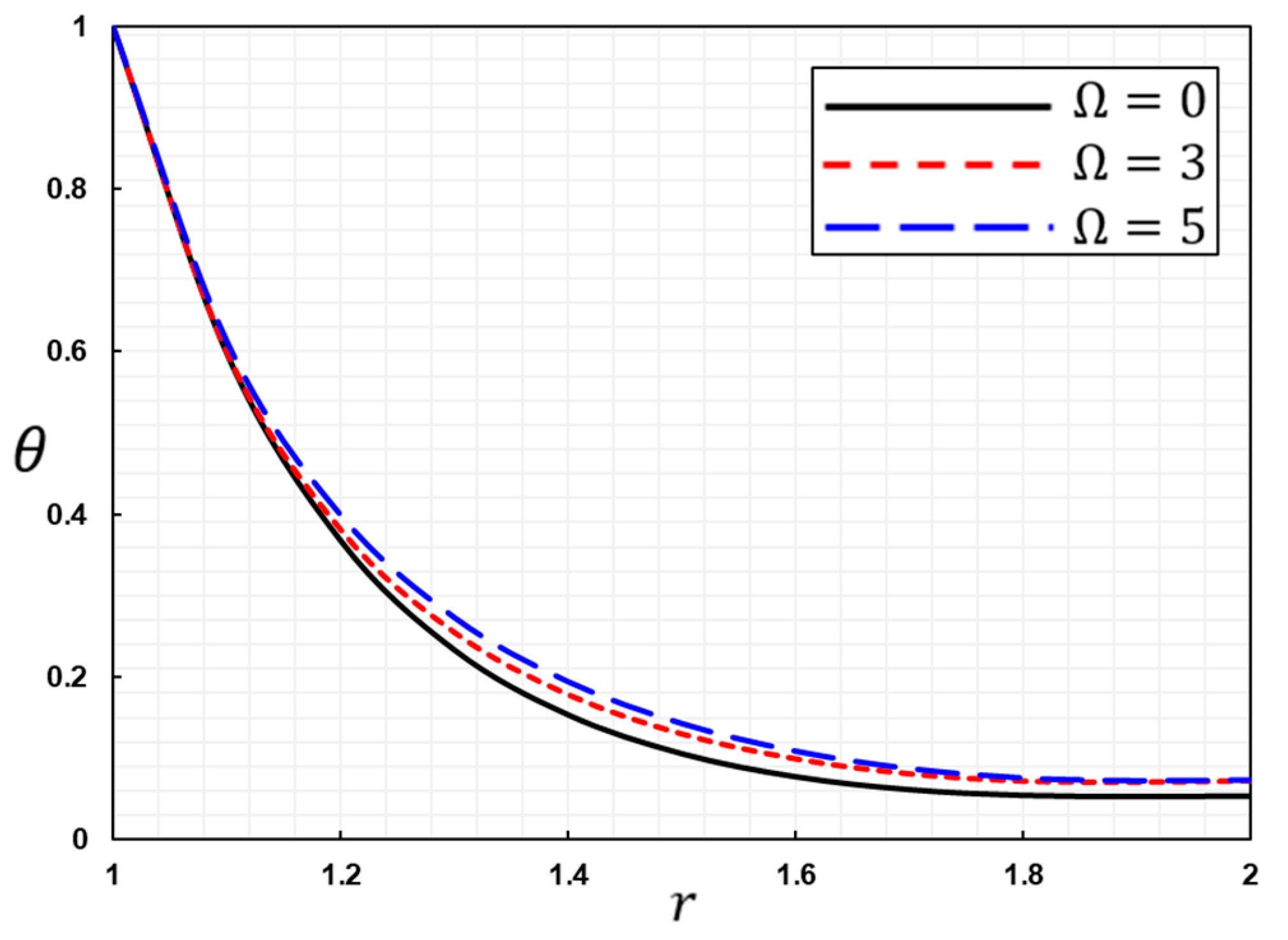
7.3. The Influence of Rotation
In problems of thermoelasticity, it often seems that the investigation of the spread of planar thermoelastic waves in rotational media may receive little attention. In general, the topic of the vibration response of flexible rotating structural systems, including beams, discs, and membranes, has not been covered in the literature published so far. However, when we consider how fast most large objects, such as the Earth, the Moon, and other planetary systems, rotate, it is more likely that thermoplastic or thermoelastic waves can move through rotating matter with thermal relaxation. The present article obtained the equation of motion, which is more general for the spread of coupled thermal and electromagnetic waves in a rotating cylindrical solid and which includes the output forces due to the effect of rotation.
To our knowledge, thermomagnetic waves generated by the modified MGTTE thermoelastic model in the rotating medium have not been studied. This is what the current subsection intends to analyze. For this reason, in this scenario, how different non-dimensional physical fields change in response to the spin parameter change will be investigated in the context of the MGTTE-thermoelastic theory involving relaxation time. It was taken into account that other effective parameters, such as pulse time
, relaxation time
, and axial magnetic field parameter
, remain constant throughout the numerical calculations. A graphic representation of the numerical results for the different domains can be seen in
Figure 16,
Figure 17,
Figure 18,
Figure 19,
Figure 20,
Figure 21 and
Figure 22.
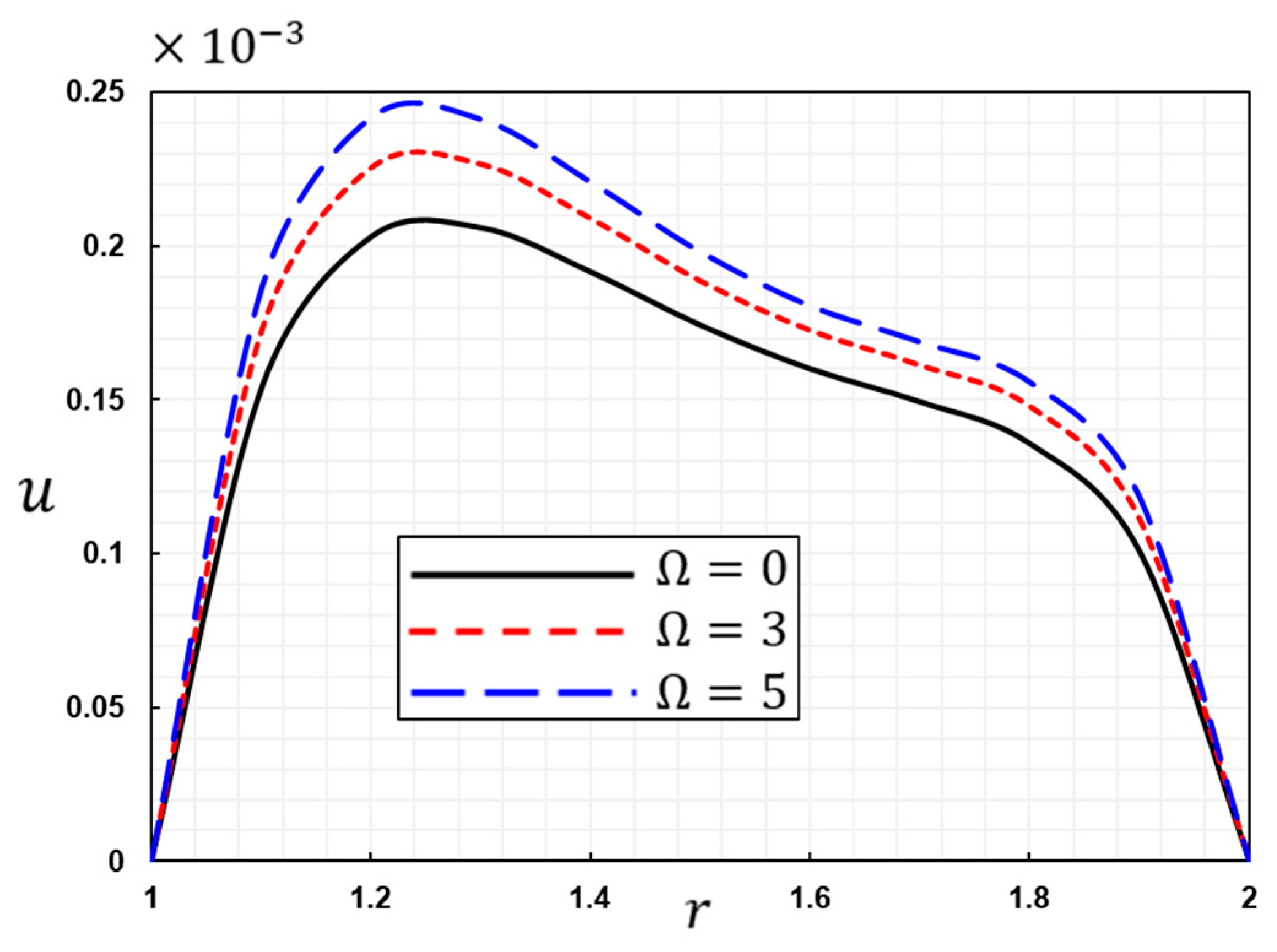
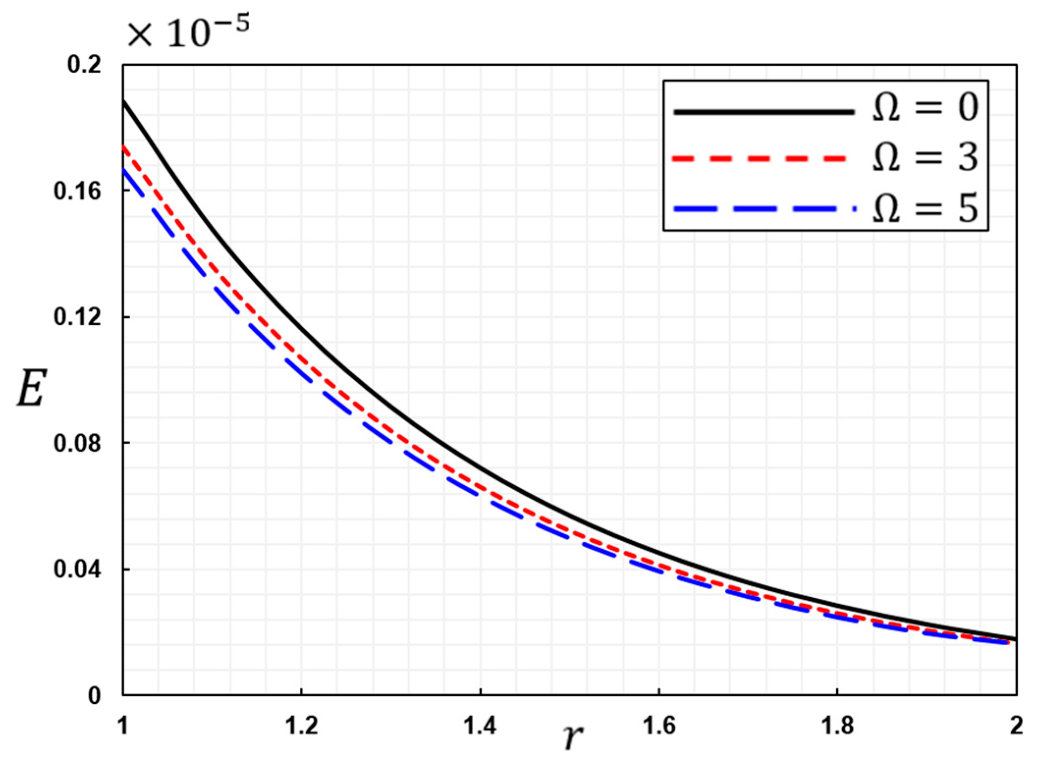
In the case of rotation, and will be taken, and in the case of non-rotation, we put the value . It can be noted from the figures that when the different mechanical distributions are taken into account, we see that thermomechanical waves travel through the solid at a confined rate. The rotating comparison point causes the material to respond as if it were distributed and deformable because gravitational acceleration and Coriolis are included in the system of equations. It is clear that the rotating terms, Coriolis and centrifugal acceleration, modify the motion equation and Maxwell’s equations, as well as Ohm’s law.
It is evident from
Figure 16 that the rotational velocity
has a small influence on the temperature variation. The temperature difference becomes smaller as time passes and the distance from the heat source grows. As can be observed in
Figure 17, the fluctuation of the displacement,
, correlates to the varied values in the rotation index
. We also see that displacement increases as rotation increases. Raising the rotation coefficients lowers displacement significantly. In addition,
Figure 17 demonstrates that the beginning points of the displacement profile for
correspond to a zero value, which conforms to the imposed boundary conditions. After that, it climbs to the highest value and then drops steadily until it reaches zero.
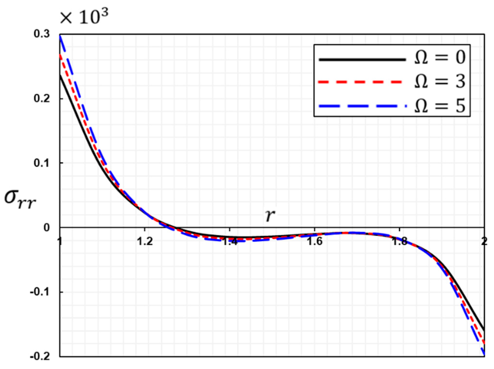
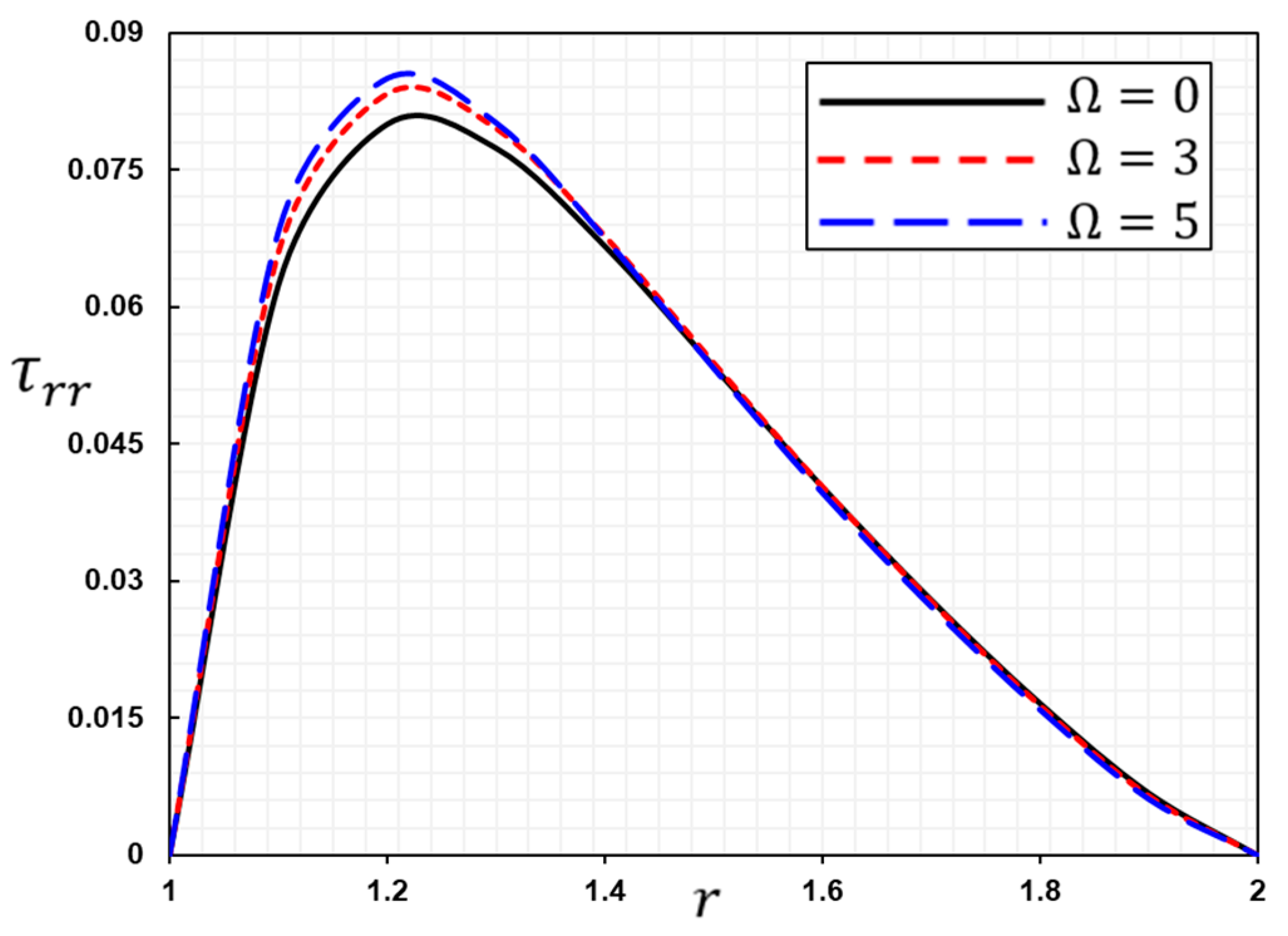
Figure 18 depicts the fluctuation of thermal stress,
, versus the radius,
, and various rotation parameters. We can observe that the rotational speed coefficient,
, has a considerable impact on the distribution of radial stress,
. As can be seen in
Figure 18, the curve of the thermal stress,
, reaches its greatest value at the boundary
, then gradually declines with the increasing radial distance until the steady state is attained. The thermal stress,
, rises as the parameter,
, rises between
and
, then reduces between
and
and then rises again between
and
.
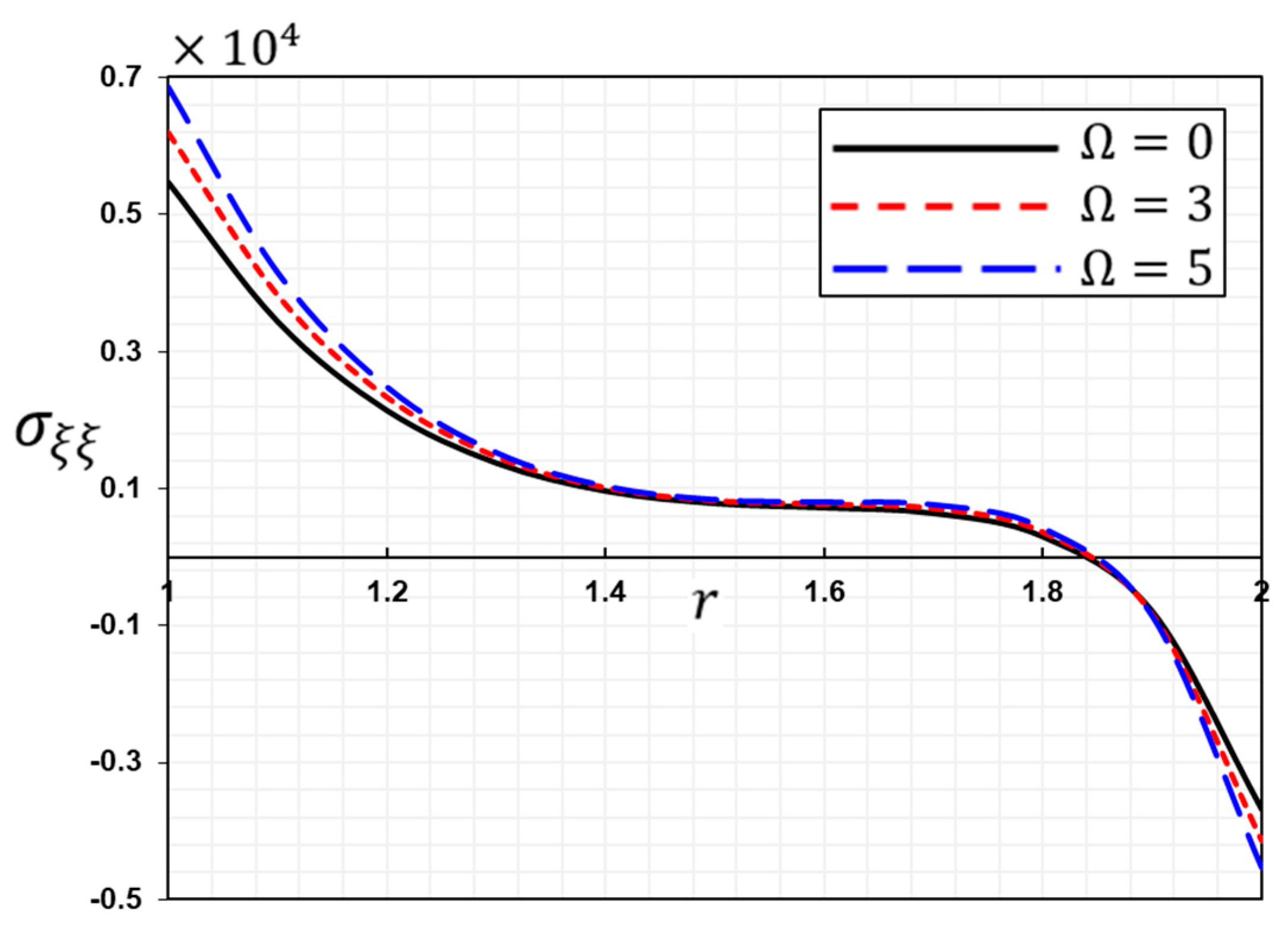
Figure 19 shows how the speed of rotation affects the hoop stress field,
, in three different situations. There is decreasing hoop stress with a larger radius,
. The hoop stress,
, is also greatly influenced by the angular velocity factor. It is evident from the graph that the stress,
, curves increase with increasing rotational speed,
, in the first period of thickness and decrease in the last period.
Figure 20,
Figure 21 and
Figure 22 depict the fluctuation in the induced magnetic field
, the induced electric field
, and the radial Maxwell stress
corresponding to the modified Ohm’s law and thermal shock for various rotating speed parameter
values. All field variables are analyzed for the variation caused by the various parameters of rotation speed. Away from the inner and outer boundary of the solid, the effect of the angular velocity,
, is shown on the induced magnetic field,
, and Maxwell’s radial stress,
, while the effect of rotation,
, is evident along the radius of the cylinder on the induced electric field,
E.
In addition to the huge structural applications of smart materials, such as thermoelastic, piezoelectric, or thermoelectric mediums, waves traveling in the presence of rotation have attracted the attention of many investigators.
8. Conclusions
In this work, the effect of the improved Moore–Gibson–Thompson model of thermoelasticity (MGTTE) on the thorough characterization of thermally generated and mechanical vibrations of transversely thermoelastic materials was investigated. Using the expanded Ohm’s law, Lord Shulman’s theory (LS), and Green–Naghdi type III, the mathematical formula for the newly proposed model was formulated (GN-III). The conventional thermoelasticity model, the extended Lord-Shulman model, and Green–Naghdi types II and III could be derived as instances.
As an illustration of the new model, the issue of a rotating long hollow cylinder with isotropic transverse characteristics, a limited inner surface, and thermal shock was explored. Moreover, the outside was fixed and thermally insulated. The solid, hollow cylindrical shell with rounded edges rotated about its axis of symmetry with a constant angular velocity. The Laplace transform method calculated physical fields by solving the system’s governing equations. In order to facilitate discussion and comparison, graphs and tables showing the deformation fields, temperature fluctuations, and distribution of thermal stresses, as well as produced electromagnetic fields, were shown.
Findings from this study suggest that changes in the analyzed field variables were significantly influenced by the applied axial magnetic field and rotation through the use of thermoelastic materials. On the other hand, its effect on the nondimensional temperature was quite small. The conventional thermoelastic theory assumes that thermal waves propagate through a transversely isotropic material at infinite velocities, while the larger Moore–Gibson–Thompson thermoelasticity model assumes that they propagate at finite velocities. Additionally, convergence and similarity between the GN-III and CTE models were observed, demonstrating the validity and application of the given thermoelasticity models. Furthermore, it could be seen that the calculated values of both the LS and MGTE systems yield similar results and behave similarly. The reason for this was the thermal relaxation time.
In conclusion, the many thermodynamic issues covered in this article have solutions that can be implemented using the methods that were presented. These findings will prove useful to scientists and theorists working in this field.


