
A Collection of Two-Dimensional Copulas Based on an Original Parametric Ratio Scheme

Department of Mathematics, LMNO, University of Caen, 14032 Caen, France
Symmetry 2023, 15(5), 977; https://0-doi-org.brum.beds.ac.uk/10.3390/sym15050977
Submission received: 3 April 2023
/
Revised: 20 April 2023
/
Accepted: 23 April 2023
/
Published: 25 April 2023
(This article belongs to the Special Issue Symmetry in Statistics and Data Science)
Abstract
:The creation of two-dimensional copulas is crucial for the proposal of novel families of two-dimensional distributions and the analysis of original dependence structures between two quantitative variables. Such copulas can be developed in a variety of ways. In this article, we provide theoretical contributions to this subject; we emphasize a new parametric ratio scheme to create copulas of the following form: , where b is a constant and is a two-dimensional function. As a notable feature, this form can operate an original trade-off between the product copula and more versatile copulas (not symmetric, with tail dependence, etc.). Instead of a global study, we examine seven concrete examples of such copulas, which have never been considered before. Most of them are extended versions of existing non-ratio copulas, such as the Celebioglu–Cuadras, Ali-Mikhail-Haq, and Gumbel–Barnett copulas. We discuss their attractive properties, including their symmetry, dominance, dependence, and correlation features. Some graphics and tables are given as complementary works. Our findings expand the horizons of new two-dimensional distributional or dependence modeling.
1. Introduction
In [1,2], Sklar introduced the concept of copula and established the main theorem that now bears his name. In the two-dimensional (2D) case, a copula is the 2D function that connects a 2D cumulative distribution function (CDF) to its marginal CDFs. In more detail, if is a random vector with CDF , and with marginal CDFs and , respectively, then there exists a 2D copula such that , . Thus, measures the connection that exists between and , as well as the (stochastic) dependence between X and Y; the independence case corresponds to the product copula . The following definition puts the mathematical basis of a 2D copula in an absolutely continuous setting.
Definition 1.
where the mixed derivative is supposed to exist almost everywhere.
In the setting of the absolutely continuous case, a 2D copula is a differentiable 2D function , satisfying the following properties:
- Boundary (B) properties: For any , we have , and ,
- Positive mixed partial derivative (PMPD) property: For any , we have
Examples include the Ali-Mikhail-Haq (AMH), Farlie–Gumbel–Morgenstern (FGM), Galambos, Gumbel–Barnett (GB), Marshall–Olkin, Plackett, Cuadras–Augé, Raftery, Brownian motion, Bertino, Celebioglu–Cuadras (CC) and Andronov copulas. We refer to [3,4] for a complete and solid overview of the topic foundation.
The research on copula is currently ongoing, and what follows is only a short overview of recent works. On the basis of copulas, the authors in [5] suggested a 2D inverse Weibull distribution and its use in a special risk model. The authors in [6] described a method for a 2D hydrologic correlation analysis using a Bayesian model-averaging copula. The authors in [7] introduced a new class of 2D FGM copulas. The authors of [8] created a novel family of 2D copulas using a unit Weibull distribution distortion. Several families of copulas are related to one another, as established in [9]. Two generalized 2D FGM copulas were elaborated in [10]. The authors in [11] highlighted a class of bivariate 2D copula transformations. An extension of the GB copula was developed in [12]. The authors in [13] elaborated on a new 2D copula via the Rüschendorf method. The authors in [14] developed and presented applications for 2D copulas using the counter-monotonic shock method. Based on the FGM copula, the authors in [15] proposed a 2D generalized half-logistic distribution and its application to household financial affordability in KSA. The author of [16] proposed a new collection of new trigonometric and hyperbolic FGM-type copulas. On the other hand, copulas have been shown to be effective in a variety of important fields, including economics, medicine, civil engineering, social science, and environmental science (see [17,18,19]).
A branch of copula theory involves developing new and original 2D copulas to provide new 2D models for dealing with the diverse dependence structures emerging from contemporary data. Beyond the norm, interesting copula functionalities have emerged, opening up new avenues for research. Among them, we may mention the trigonometric copulas that are able to model circular-type dependencies (see [20,21,22]), and the ratio-type copulas that can be considered understudied beyond the classical schemes (see [23,24,25,26,27], among others). The findings of this article contribute to this last aspect; we offer original copulas of the following parameter–ratio form:
where b denotes a certain constant and represents a certain function satisfying , among other properties to be specified. This function may also depend on some parameters. The form in Equation (1) is derived from the AMH copula, a paragon of the Archimedean family. We recall that it is defined with and , with , or equivalently, with , with . The interests of the form in Equation (1) are: (i) when , we have ; we thus rediscover the benchmark product copula (the same remark holds if we may have ), and (ii) if we choose , where denotes a certain copula, then, by taking , the copula in Equation (1) corresponds to . As a result, the parameter b operates an original trade-off between the product copula and . In this sense, the copula can be viewed as a one-parameter ratio-generalization of and, thus, as a flexibly modified version. Another viewpoint is that can be written as or , where and . These secondary functions thus perturb the product copula. The idea of perturbing the functionalities of the product copula is not new (see [28,29], and the references therein), but the considered weighted ratio form for remains the original angle of the article.
Due to the mathematical complexity of the form in Equation (1), a general study is nearly impossible. For this reason, we exhibit a collection of seven copulas of this form with various functions , mainly of polynomial, exponential, and logarithmic types. The behavior of may be affected by additional parameters. For each of them, admissible ranges of values are determined. All the copulas presented are new in the literature, and most of them are well-referenced extended ones. The proofs are detailed and self-contained. In them, the main tedious point remains the PMPD property, which necessitates technical differentiation developments and prudent factorization. For each proposed copula, we examine their properties, including shapes, varied symmetry, dependence, and correlations. In particular, their shapes are shown graphically, and tables of values are given for some correlation measures. Among the main findings, we elaborate on a three-parameter extended version of the AMH copula, making it more flexible and adaptable in a statistical sense. In view of the existing theoretical and applied works on the AMH copula (see [30,31,32], among others), the potential of interest of this extension is certain.
2. Original Ratio-Type Copulas
This section presents seven original ratio-type copulas of the form in Equation (1), each defined with a specific function .
2.1. First Copula
The first copula considers the form in Equation (1) with the 2D one-parameter logarithmic function .
Proposition 1.
Let be the following 2D function:
Then, for and , is a 2D copula.
Proof.
First, can be written as
where . Thus, the conditions and imply that . Let us prove that, under this modified form, is a 2D copula based on Definition 1.
- On the B property: For any , we haveand, in a similar way, . Since , it is immediate that and . The B property is proved.
- On the PMPD property: Applying several differentiation rules and factorizing in a way to be able to conclude, we haveFor any , we have , and since , we have , and all of the main terms in the above equations are non-negative. Therefore, we haveand the PMPD property is established.
This ends the proof. □
Remark 1.
In Proposition 1, the value implies no role for b; we have . The interrogative case and is excluded.
The copula defined in Equation (2) is called the original ratio-type 1 (OR1) copula. As far as we know, it is a new addition to the literature and is one of the few copulas that involves a product of logarithmic terms in the denominator. Let us now connect it with some existing copulas. To begin, as mentioned in Remark 1, it corresponds to the product copula when , i.e., . Furthermore, based on the inequality for any , we have for any , and the following copula dominances hold:
where is the AMH copula defined by
with .
Clearly, for , has the same form as the AMH copula, except that the separable polynomial function is replaced by the separable two-logarithmic function . In this sense, the OR1 copula can be viewed as a natural two-logarithmic extension of the AMH copula. On the other hand, copula dominance results, as in Equation (3), are important to have information on the quadrant dependence and to compare the correlation properties of the involved copulas. This is especially true for the Spearman correlation measure (to be presented later). For instance, based on Equation (3), we can say that the OR1 copula is negatively quadrant dependent and has negative Spearman correlation measure values that are lower than those associated with the AMH copula.
Concerning its main properties, the OR1 copula is diagonally symmetric and, for , it is not radially symmetric, is not Archimedean, and has no tail dependence. It has the following medial correlation measure (also called Blomqvist beta):
It is always negative; the OR1 copula is designed to model negative correlations. The Spearman correlation measure is given by the following integral expression:
It does not have a closed-form expression. As a numerical study, Table 1 presents some of its values for several admissible values of a and b.
This table confirms that the OR1 copula is adapted to model the negative dependence, and, for the considered parameter values, we have .
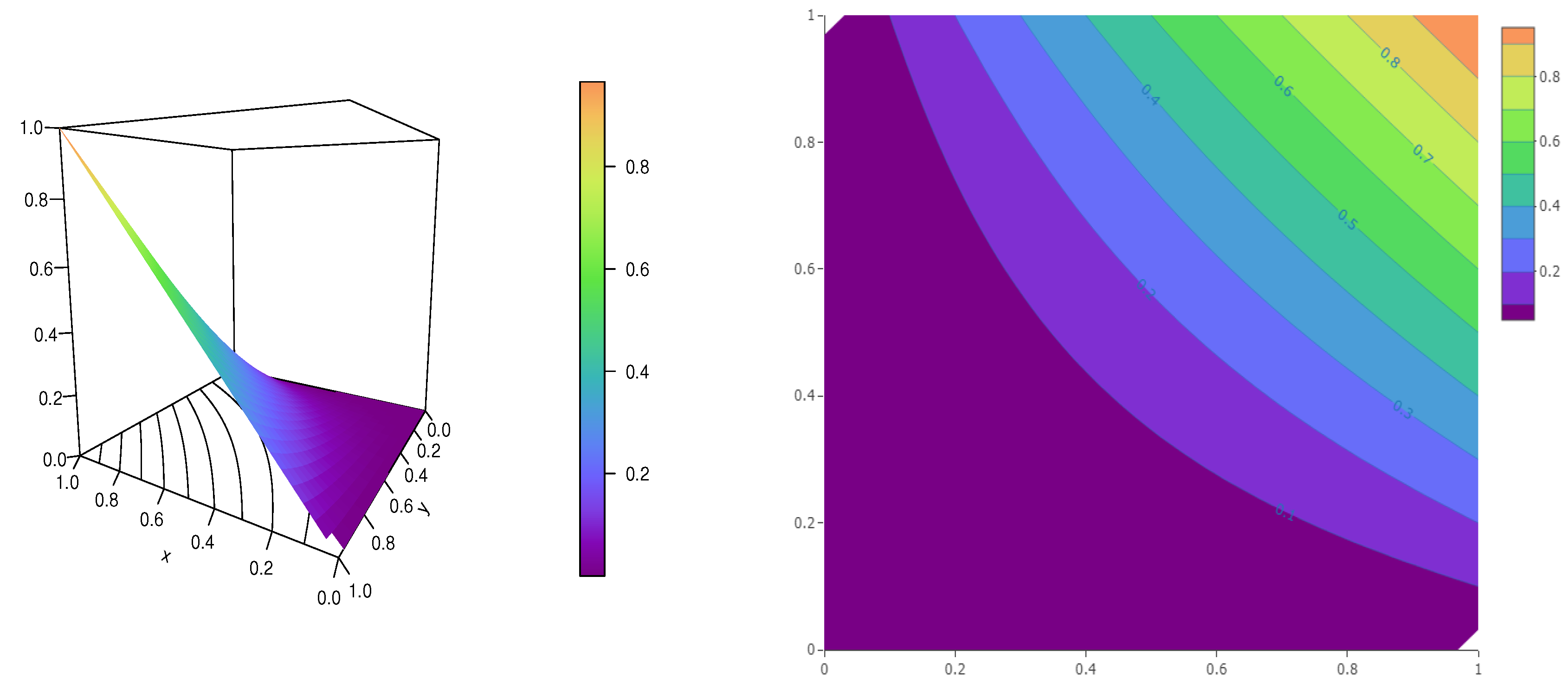
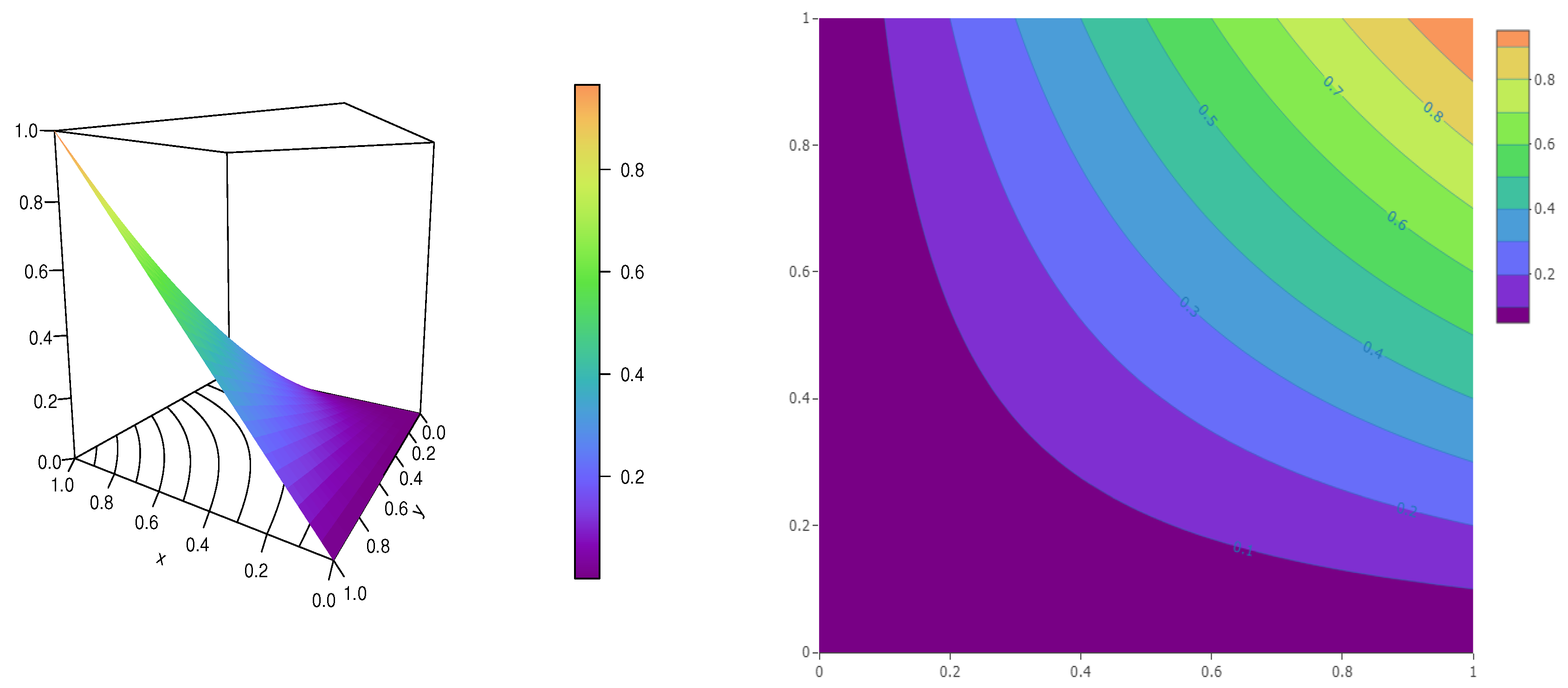
For illustrative purposes and visual validation, with the use of the free software R (see [33]), Figure 1 shows two complementary plots of the OR1 copula for and .
We observe the typical shapes of a copula, with the clear fact that the OR1 copula is valid. As a last result, the OR1 copula satisfies the Fréchet–Hoeffding inequalities: for any , we have , which can also be expressed as
(It is understood, for and ). It is not claimed that these inequalities are sharp, but 2D inequalities remain relatively rare and important, so that they can find interest in diverse multivariate analysis settings.
2.2. Second Copula
The second copula considers the form in Equation (1) with the 2D one-parameter polynomial-logarithmic function ; in comparison to the previously considered , the term has replaced .
Proposition 2.
Let be the following 2D function:
Then, for and , is a 2D copula.
Proof.
First of all, can be written as
where . Hence, the conditions and imply that . Let us prove that, under this simplified form, is a 2D copula based on Definition 1.
- On the B property: For any , we haveand
- Since , it is immediate that and, similarly, since for , we have . This proves the B property.
- On the PMPD property: Combining various differentiation rules and factorizing in a way that allows us to draw conclusions, we haveFor any , we have and, since , we haveHence, all of the main terms in the above equations are non-negative. Therefore, we haveThe PMPD property holds.
The proof is complete. □
Remark 2.
In Proposition 2, the value implies no role for b; we have . The interrogative case and is excluded.
The copula defined in Equation (5) is named the original ratio-type 2 (OR2) copula. As far as we are aware, it has never been brought up in the literature. Now, let us link it to some existing copulas. To begin, referring to Remark 2, it corresponds to the product copula when , i.e., . Furthermore, for any , since , the following copula dominances hold:
where is the OR1 copula as defined in Equation (2) and is described in Equation (4). For , has the same denominator term as the AMH copula, except that the separable polynomial function is replaced by the separable polynomial–logarithmic function . In this sense, it can be viewed as a modification, and as a trade-off between the OR1 and AMH copulas.
Concerning its main properties, for , the OR2 copula is not diagonally symmetric, radially symmetric, or Archimedean, and has no tail dependence. Its medial correlation measure is
It is, of course, always negative; the OR2 copula is designed to model negative correlations. The Spearman correlation measure does not have a closed-form expression, motivating numerical work. Table 2 presents some of its numerical values for several admissible values of a and b.
Thus, we have , which is acceptable, and this table confirms that the OR2 copula is adjusted to model negative dependence.
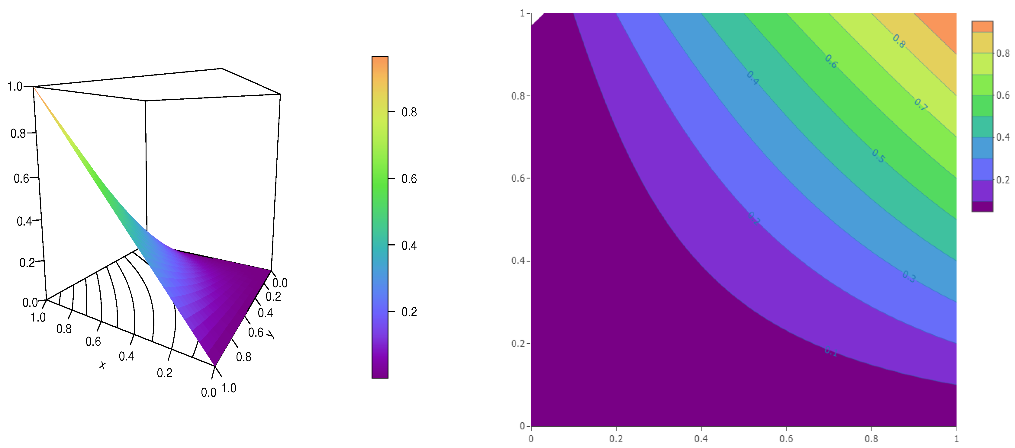
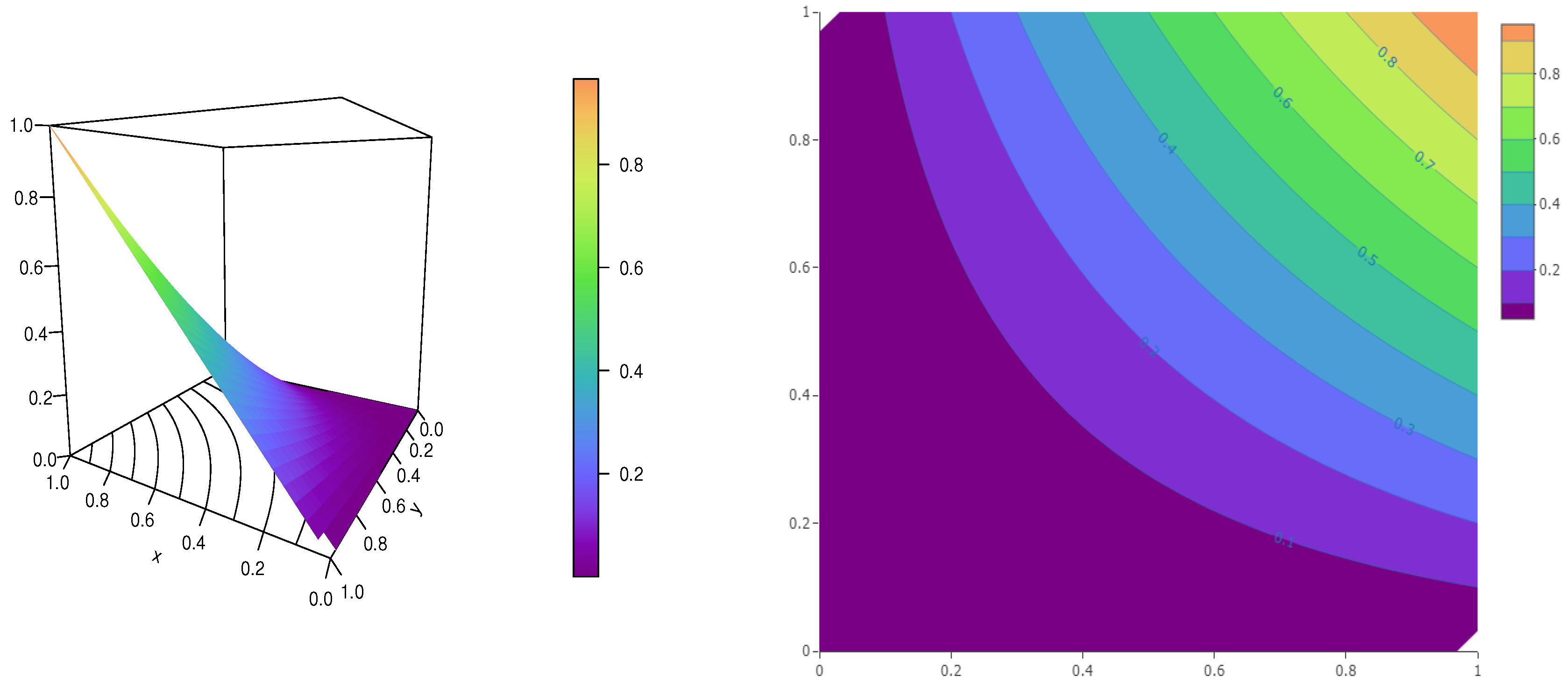
For illustrative purposes and visual validation, Figure 2 displays the plots of the OR2 copula for and .
We observe the typical shapes of a copula, given the clear fact that the OR2 copula is valid.
One final copula fact is that the OR2 copula satisfies the Fréchet–Hoeffding inequalities, implying that, for any ,
These inequalities can find applications in diverse multivariate analysis settings.
2.3. Third Copula
The third copula considers the form in Equation (1) for the 2D one-parameter exponential function , which is of a completely different nature to the two previously considered functions .
Proposition 3.
Let be the following 2D function:
Then, for and , is a 2D copula.
Proof.
Let us demonstrate that is a 2D copula based on Definition 1.
- On the B property: For any , we haveand, similarly, we have . On the other hand, we haveand, similarly, we have . The B property is demonstrated.
- On the PMPD property: By differentiating and factorizing in a way that allows us to draw conclusions, we haveLet us investigate a sharp lower bound for the term , which appears two times. For any , we haveand, on the other hand,So . Therefore, we have . Since the exponential terms are non-negative and , we haveFor any , since , it is clear thatand, since , we haveCombining the above inequalities, we obtainThe PMPD property is, thus, satisfied.
This ends the proof. □
The copula defined in Equation (6) is named the original ratio-type 3 (OR3) copula.
It is worth noting that, for , the OR3 copula is reduced to the product copula, and, for , it becomes
which corresponds to the CC copula established in [34,35]. See also [36].
Owing to the inequality for any , we have for any and , implying the following copula dominance:
where is the AMH copula defined in Equation (4) with (instead of c).
Certain power series of the OR3 copula can be established. For instance, for any , , and , it follows from the geometric and binomial series that
One can observe that it is an infinite series involving the CC copula with a varying parameter. Such series expansion can be used for various analytical purposes (expansions of correlation measures, calculus of moments, etc.).
The main properties are now investigated. The OR3 copula is diagonally symmetric, and, for , it is not radially symmetric, is not Archimedean, and has no tail dependence.
Furthermore, the OR3 copula has the following medial correlation measure:
It is negative for , and non-negative for ; the OR3 copula can model various types of correlations. There is no closed-form expression for the Spearman correlation measure. For an idea of its numerical behavior, we calculate it for several admissible values of a and b and collect the results in Table 3.
The obtained range of values for is . This shows that the OR3 copula is adjusted to model weak or moderate negative or positive dependence.
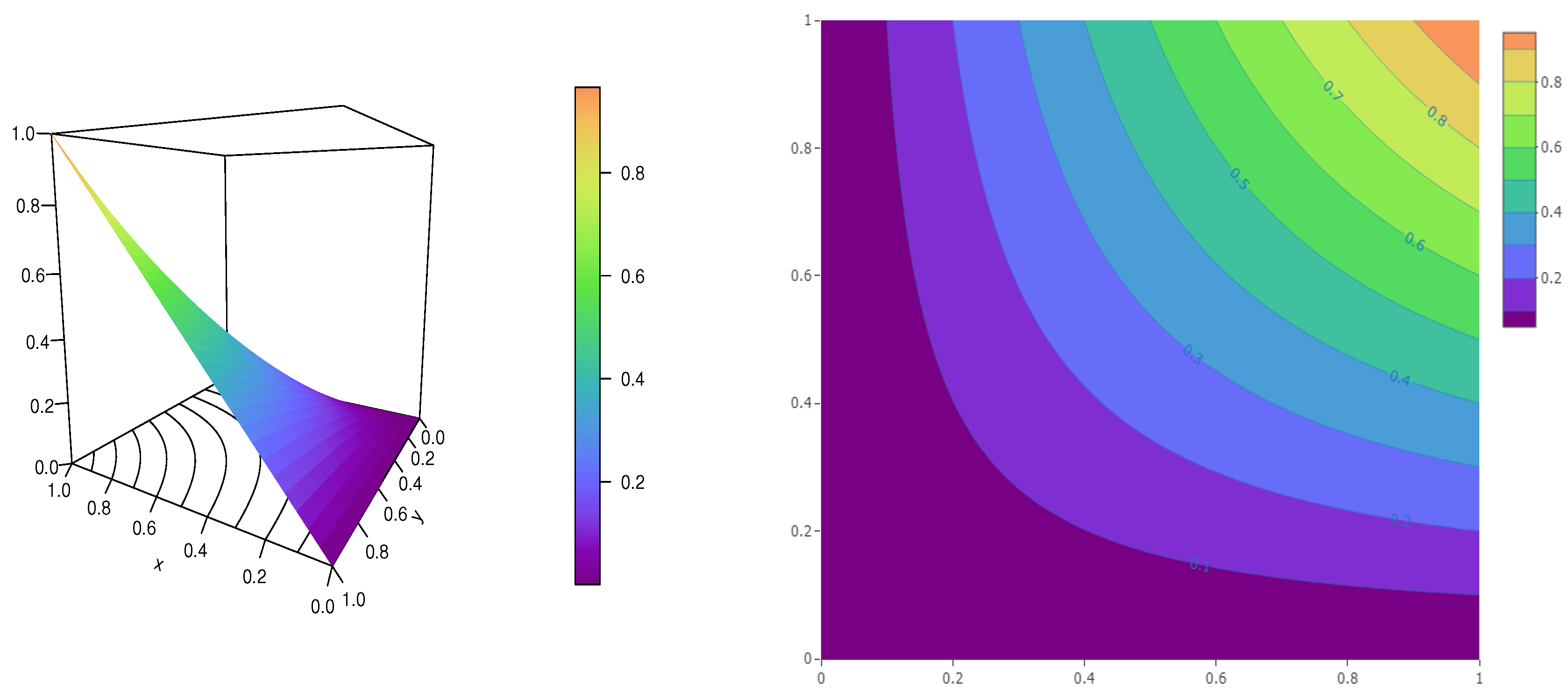
For illustrative purposes and visual validation, Figure 3 displays some plots of the OR3 copula for and .
We see the standard copula shapes while also observing that the OR3 copula is valid.
As a last copula fact, the OR3 copula satisfies the Fréchet–Hoeffding inequalities, and so, for any , we have
These inequalities can be used in a variety of multivariate analysis contexts.
2.4. Fourth Copula
The fourth copula considers the form in Equation (1) with the 2D one-parameter ratio–polynomial function .
Proposition 4.
Let be the following 2D function:
Then, for and , is a 2D copula.
Proof.
Since, for , we have
we can restrict our attention to the case instead of . Thus, under this condition, let us prove that is a 2D copula based on Definition 1.
- On the B property: For any , we haveand, similarly, we have . On the other hand, we haveand, similarly, we have . The B property is proved.
- On the PMPD property: Using several differentiation and factorization strategies, we establishwhereLet us focus on the term A, which is the main interrogative of its sign. For any , since and , we haveFurthermore, since and , all of the other main terms are immediately non-negative. Therefore, we haveThe PMPD property is established.
The desired result is obtained. □
The copula defined in Equation (7) is named the original ratio-type 4 (OR4) copula. As an immediate remark, for , it is reduced to the product copula. An alternative form of the OR4 copula is
In particular, for , it is reduced to
which is a special case of a ratio copula described in [37].
Now, let us remark that, for any , we have , which implies that . As a result, the following copula dominance holds:
The main properties of the OR4 copula are now listed. To begin with, it is diagonally symmetric and, for , it is not radially symmetric, is not Archimedean, and has no tail dependence. The associated medial correlation measure is given by
This measure is always positive; the OR4 copula is adapted to model positive correlations. The Spearman correlation measure does not have a closed-form expression. As a numerical work, Table 4 presents some of its numerical values for several admissible values of a and b.
Hence, for the considered parameter values, we have . This confirms that the OR4 copula is adjusted to model moderate positive dependence.
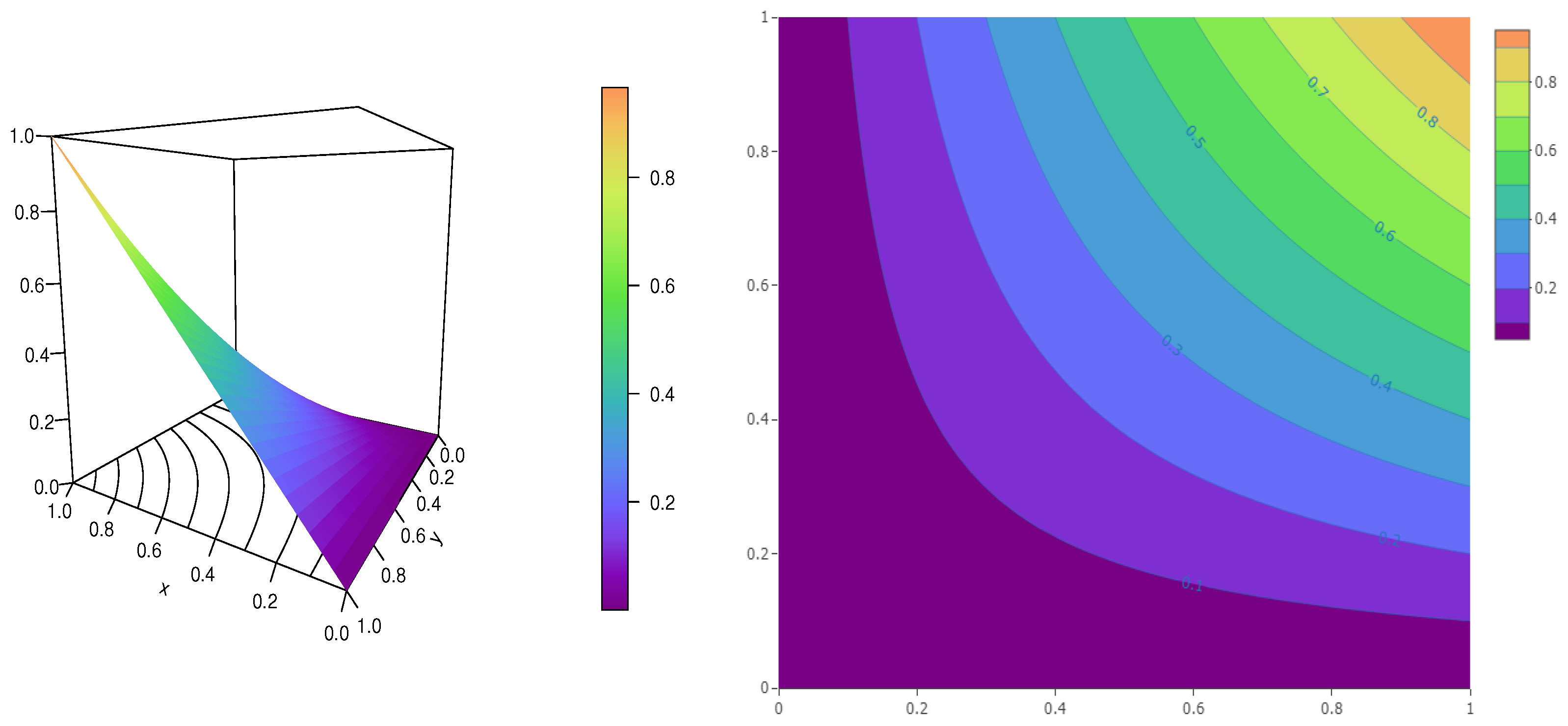
For illustrative purposes and visual validation, Figure 4 displays some plots of the OR4 copula for .
We observe the typical shapes of a copula, given the clear fact that the OR4 is valid.
As a last copula fact, the OR4 copula satisfies the Fréchet–Hoeffding inequalities. Hence, for any , we have
These inequalities can find applications in diverse multivariate analysis settings.
2.5. Fifth Copula
The fifth copula can be viewed as complementary to the OR4 copula; we consider the form in Equation (1) with the 2D one-parameter ratio–polynomial function , corresponding to the exact inverse function of the previous section.
Proposition 5.
Let be the following 2D function:
Then, for and , is a 2D copula.
Proof.
Since, for , we have
we can restrict our attention to the case instead of . Thus, under this condition, let us prove that is a 2D copula based on Definition 1.
- On the B property: For any , we haveand, similarly, we have . On the other hand, we haveand, similarly, we have . This proves the B property.
- On the PMPD property: Differentiating and arranging the obtained terms in a manageable way, we obtainFor any , since and , all of the main terms are immediately non-negative. Therefore, we haveThe PMPD property is thus satisfied.
This ends the proof. □
The copula defined in Equation (9) is named the original ratio-type 5 (OR5) copula. For , it is reduced to the product copula. An alternative form of the OR5 copula is
In particular, for , it is reduced to
Because we have for any , we have . As a result, the following copula dominance holds:
We now list the key characteristics of the OR5 copula. To begin, it is diagonally symmetric, and, for , it is not radially symmetric, is not Archimedean, and has no tail dependence. The associated medial correlation measure is given by
It is always negative; the OR5 copula is designed to model negative correlations. The Spearman correlation measure does not have a closed-form expression. As an indicator, Table 5 presents some of its numerical values for several admissible values of a and b.
For the selected parameter values, we see that , which is acceptable in terms of range. Thus, the OR5 copula can be chosen to model negative dependence.
For illustrative purposes and visual validation, Figure 5 displays some plots of the OR5 copula for .
This figure clearly demonstrates the validity of the OR5 copula.
As the other copulas, the OR5 copula satisfies the Fréchet–Hoeffding inequalities. Thanks to them, for any , the following inequalities hold:
They can find applications in diverse multivariate analysis settings.
2.6. Sixth Copula
The sixth copula aims to generalize the AMH copula; we consider the form in Equation (1) with the 2D two-parameter polynomial function .
Proposition 6.
Let be the following 2D function:
Then, for , , and one of the following cases for b:
- Case 1
- if ,
- Case 2
- if ,
is a 2D copula.
Proof.
The function is, thus, well defined; the extreme case where the denominator term can be equal to 0 will be discussed in Remark 3. Let us now prove that is a 2D copula based on Definition 1.
As a preliminary result, let us prove that is non-negative. For any and since , it is clear that . Let us now focus on the denominator term by distinguishing Cases 1 and 2.
- For Case 1: For any , and , since , we have
- For Case 2: For any , and , since , we have
- On the B property: For any , we haveand, similarly, we have . On the other hand, we haveand, similarly, we have . The B property is demonstrated.
- On the PMPD property: Let us distinguish Cases 1 and 2.
- For Case 1: By combining several differentiation rules and factorizing in a way to be able to conclude, we havewhereLet us focus on the term A, which is the main interrogative of its sign. For any , since and , we have and . As a result, since , we haveFurthermore, since and , all of the other main terms are immediately non-negative. Therefore, we have
- For Case 2: With the same differentiation as that of Case 1, but a completely different factorization, we obtainwhereLet us focus on the term B, which is the main interrogative of its sign. For any , since and , we havewhich is non-negative. Furthermore, since and , we have . As a result, since , we haveOn the other hand, since and , all of the other main terms are immediately non-negative. As a result, we findHence, for Cases 1 and 2, the PMPD property holds.
The proof is now complete. □
Remark 3.
In Proposition 6, the values or imply no role for b; we have . The interrogative cases or and are excluded.
Remark 4.
Since , eventually, Cases 1 and 2 can be replaced by the more restrictive but unique condition: .
The copula defined in Equation (10) is named the original ratio-type 6 (OR6) copula. For or , it is reduced to the product copula. For and , it is reduced to the AMH copula as defined in Equation (4) with . All the other parameter values give a new copula, as far as we know. In particular, for , the following original expression is obtained:
Various copula dominance results can be established. The most significant one is based on the generalized Bernoulli inequality with a power exponent in the range of (see [38]). This inequality gives , which implies that
where is given in Equation (4) with the constant (instead of c).
Concerning its main properties, the OR6 copula is diagonally symmetric. For , it is not radially symmetric. For and , it is not Archimedean. In addition, it has no tail dependence except for the cases , , and , where a left-tail dependence is established. It has the following medial correlation measure:
which is negative for , and negative for ; the OR6 copula is designed to model negative or positive correlations. The Spearman correlation measure does not have a closed-form expression. As a numerical indicator, Table 6 presents some of its numerical values for several admissible values of a, b, and c.
Hence, for the considered parameter values, we have . Thus, the OR6 copula is designed to model negative or positive dependence.
For illustrative purposes and visual validation, Figure 6 displays some plots of the OR6 copula for .
This figure clearly demonstrates the validity of the OR6 copula. Indeed, we observe the typical shapes of a copula.
As a last copula fact, the OR6 copula satisfies the Fréchet–Hoeffding inequalities, and as a result, for any , we have
These inequalities can find applications in diverse multivariate analysis settings.
2.7. Seventh Copula
The seventh and last copula of the list can be viewed as a two-logarithmic version of the OR3 copula; we consider the form in Equation (1) with the 2D one-parameter exponential logarithmic function .
Proposition 7.
Let be the following 2D function:
Then, for and , is a 2D copula.
Proof.
Let us prove that is a 2D copula based on Definition 1.
- On the B property: For any , we haveand, similarly, we have . On the other hand, since , we haveand, similarly, we have . The B property is established.
- On the PMPD property: With appropriate differentiation techniques and factorizing in a way to be able to conclude, we havewhereLet us focus on A, which is the main interrogative of its sign. For any , we have and . Furthermore, since and , we have andOn the other hand, since and , all of the other main terms are immediately non-negative. As a result, we haveThis demonstrates the PMPD property.
This ends the proof. □
The copula defined in Equation (11) is named the original ratio-type 7 (OR7) copula. For , it is reduced to the product copula, and, for , it becomes
which corresponds to the GB copula.
Owing to the inequality for any , we have for any and , implying the following copula dominance:
where is the OR1 copula defined in Equation (2).
Concerning its main properties, the OR7 copula is diagonally symmetric and, for , it is not radially symmetric, is not Archimedean, has no tail dependence, and has the following medial correlation measure:
This measure is always negative; the OR7 copula is designed to model negative correlations. The Spearman correlation measure does not have a closed-form expression. For information, Table 7 presents some of its numerical values for several admissible values of a and b.
In our setting, we have , showing that the OR7 copula is able to model negative dependence.
For illustrative purposes and visual validation, Figure 7 shows the standard and intensity contour plots of the OR7 copula for .
This figure clearly demonstrates the validity of the OR7 copula; the typical shapes of a copula are observed.
As a last copula fact, the OR7 copula satisfies the Fréchet–Hoeffding inequalities, from which we derive the following result: for any , we have
These inequalities can find applications in diverse multivariate analysis settings.
3. Summary, Discussion, and Perspectives
3.1. Summary
For the objectives of dependence modeling, two-dimensional copula creation is essential. In this study, we presented theoretical advances in the field and highlighted a novel parametric ratio scheme. The seven copulas elaborated on in this article are presented in Table 8.
The ideas below have been developed throughout this article.
- They are new in the literature, simple, original in form, and operational for well-identified parameter values; it is, however, not claimed that the given ranges of values are the optimal ones.
- They generalize well-known copulas, making them more flexible in terms of functionalities. In particular, the OR3, OR6, and OR7 copulas generalize the CC, AMH and GB copulas, respectively.
- They benefit from attractive properties, such as symmetric, dependent, dominant, and correlation features.
3.2. Discussion
Thus, we focused on special copulas of the parameter–ratio form given in Equation (1). As noticed in the proofs of some results, as in the proofs of Propositions 1 and 2, for instance, it is sometimes more convenient to consider the following general copula form:
where c denotes a real number and represents a certain two-dimensional function. One can remark that this form and the one in Equation (1) correspond with the following configuration: and . This general form, perhaps more connected with that of the AMH copula, could have been the subject of a similar study.
Along the article, we examined concrete, operational, and motivated examples of functions , instead of a global study based on . The reason is that the consideration of in full generality significantly complicates the developments, especially the necessary differentiations and factorizations to prove the PMPD property (see Definition 1). The investigations reveal that there is no universal factorization scheme to prove the PMPD property for all examples. The level of functional complexity is too high for a global study, according to our viewpoint. However, this challenge can perhaps be achieved through a certain analysis strategy that we actually left for future research.
Anyway, based on the general form in Equation (1), under the assumption that defines a valid copula, some results can be exhibited. For instance, one can remark that
Therefore, if for any , then , implying that , so that is negatively quadrant dependent, and if for any , the contrary holds: is positively quadrant dependent. Such properties were implicitly demonstrated for the suggested copulas of the article, often with the use of direct inequalities, and the notion of copula dominance results involving the product copula into the article (see Equations (3) and (8), for instance).
The simulation and parameter estimation of copulas are two important aspects that were not developed in the article. For these aspects, we can consider using standard methods that have demonstrated their efficiency for most well-established copulas, as described in [4]. In particular, for the parameter estimation, we can perform the omnibus estimation method elaborated in [39], among others.
3.3. Perspectives
Other copulas can be immediately derived from those proposed, such as the corresponding survival, x-flipping, and y-flipping copulas (see [4]). Each of them may be of interest for specific applied scenarios involving the dependence of two quantitative variables. Moreover, we restricted our attention to the absolutely continuous case, implying differentiable functions in Equation (1), but it can be of interest to consider functions, at least for the constructions of copulas reaching the Fréchet–Hoeffding bounds. Another logical perspective of this article is the creation of copulas having a similar ratio form but with greater dimensions. Their applications for data analysis are also hot topics. A high level of knowledge is, however, required for this applied aspect, which we leave to further study.
Funding
This research received no external funding.
Institutional Review Board Statement
Not applicable.
Informed Consent Statement
Not applicable.
Data Availability Statement
Not applicable.
Acknowledgments
The author expresses gratitude to the three reviewers, the associate editor, and the editor for their constructive feedback on the article.
Conflicts of Interest
The author declares no conflict of interest.
References
- Sklar, A. Fonctions de Répartition à n Dimensions et leurs Marges; Publications de l’Institut Statistique de l’Université de Paris: Paris, France, 1959; Volume 8, pp. 229–231. [Google Scholar]
- Sklar, A. Random variables, joint distribution functions, and copulas. Kybernetika 1973, 9, 449–460. [Google Scholar]
- Nadarajah, S.; Afuecheta, E.; Chan, S. A compendium of copulas. Statistica 2017, 77, 279–328. [Google Scholar]
- Nelsen, R. An Introduction to Copulas, 2nd ed.; Springer: Berlin/Heidelberg, Germany, 2006. [Google Scholar]
- Mondal, S.; Kundu, D. A bivariate inverse Weibull distribution and its application in complementary risks model. J. Appl. Stat. 2020, 47, 1084–1108. [Google Scholar] [CrossRef] [PubMed]
- Wen, Y.; Yang, A.; Kong, X.; Su, Y. A Bayesian-model-averaging copula method for bivariate hydrologic correlation analysis. Front. Environ. Sci. 2022, 9, 744462. [Google Scholar] [CrossRef]
- Bekrizadeh, H.; Jamshidi, B. A new class of bivariate copulas: Dependence measures and properties. Metron 2017, 75, 31–50. [Google Scholar] [CrossRef]
- Aldhufairi, F.; Sepanski, J. New families of bivariate copulas via unit Weibull distortion. J. Stat. Appl. 2020, 7, 1–20. [Google Scholar] [CrossRef]
- Abd, El-Monsef, M.; Elsobky, S.; Seyam, M. The relations between some families of copulas. J. Adv. Math. Comput. Sci. 2021, 36, 31–49. [Google Scholar]
- Cuadras, C.M.; Diaz, W.; Salvo-Garrido, S. Two generalized bivariate FGM distributions and rank reduction. Commun. Stat. Theory Methods 2020, 49, 5639–5665. [Google Scholar] [CrossRef]
- Manstavičius, M.; Bagdonas, G. A class of bivariate independence copula transformations. Fuzzy Sets Syst. 2022, 428, 58–79. [Google Scholar] [CrossRef]
- Diaz, W.; Cuadras, C.M. An extension of the Gumbel-Barnett family of copulas. Metrika 2022, 85, 913–926. [Google Scholar] [CrossRef]
- Seyam, M.M.; Elsobky, S.M. New bivariate MS copula via Rüschendorf method. Inf. Sci. Lett. 2022, 11, 1087–1092. [Google Scholar]
- El Ktaibi, F.; Bentoumi, R.; Sottocornola, N.; Mesfioui, M. Bivariate copulas based on counter-monotonic shock method. Risks 2022, 10, 202. [Google Scholar] [CrossRef]
- Hassan, M.K.H.; Chesneau, C. Bivariate generalized half-logistic distribution: Properties and its application in household financial affordability in KSA. Math. Comput. Appl. 2022, 27, 72. [Google Scholar] [CrossRef]
- Chesneau, C. A collection of new trigonometric- and hyperbolic-FGM-type copulas. AppliedMath 2023, 3, 147–174. [Google Scholar] [CrossRef]
- Hui-Mean, F.; Yusof, F.; Yusop, Z.; Suhaila, J. Trivariate copula in drought analysis: A case study in peninsular Malaysia. Theor. Appl. Climatol. 2019, 138, 657–671. [Google Scholar] [CrossRef]
- Orcel, O.; Sergent, P.; Ropert, F. Trivariate copula to design coastal structures. Nat. Hazards Earth Syst. Sci. 2020, 21, 239–260. [Google Scholar] [CrossRef]
- Roberts, D.J.; Zewotir, T. Copula geoadditive modeling of anaemia and malaria in young children in Kenya, Malawi, Tanzania and Uganda. J. Health Popul. Nutr. 2020, 39, 8. [Google Scholar] [CrossRef]
- Chesneau, C. Theoretical study of some angle parameter trigonometric copulas. Modelling 2022, 3, 140–163. [Google Scholar] [CrossRef]
- Hodel, F.H.; Fieberg, J.R. Circular-linear copulae for animal movement data. Methods Ecol. Evol. 2022, 13, 1001–1013. [Google Scholar] [CrossRef]
- Hodel, F.H.; Fieberg, J.R. Cylcop: An R package for circular-linear copulae with angular symmetry. bioRxiv 2021. [Google Scholar] [CrossRef]
- Chesneau, C. A new two-dimensional relation copula inspiring a generalized version of the Farlie-Gumbel-Morgenstern copula. Res. Commun. Math. Math. Sci. 2021, 13, 99–128. [Google Scholar]
- Chesneau, C. Some new ratio-type copulas: Theory and properties. Appl. Math. 2022, 49, 79–101. [Google Scholar] [CrossRef]
- Dolati, A.; Úbeda-Flores, M. Constructing copulas by means of pairs of order statistics. Kybernetika 2009, 45, 992–1002. [Google Scholar]
- Durante, F.; Fernández-Sánchez, J.; Trutschnig, W. Solution to an open problem about a transformation on the space of copulas. Depend. Model. 2014, 2, 65–72. [Google Scholar] [CrossRef]
- Mesiar, R.; Stupňanová, A. Open problems from the 12th International Conference on Fuzzy Set Theory and Its Applications. Fuzzy Sets Syst. 2015, 261, 112–123. [Google Scholar] [CrossRef]
- Saminger-Platz, S.; Kolesárová, A.; Šeliga, M.; Mesiar, R.; Klement, E.P. New results on perturbation-based copulas. Depend. Model 2021, 9, 347–373. [Google Scholar] [CrossRef]
- Šeliga, A.; Kauers, M.; Saminger-Platz, S.; Mesiar, R.; Kolesárová, A.; Klement, E.P. Polynomial bivariate copulas of degree five: Characterization and some particular inequalities. Depend. Model 2021, 9, 13–42. [Google Scholar] [CrossRef]
- Kumar, P. Probability distributions and estimation of Ali-Mikhail-Haq copula. Appl. Math. Sci. 2010, 4, 657–666. [Google Scholar]
- Yang, Q.; Xu, M.; Lei, X.; Zhou, X.; Lu, X. A methodological study on AMH copula-based joint exceedance probabilities and applications for assessing tropical cyclone impacts and disaster risks (Part I). Trop. Cyclone Res. Rev. 2014, 3, 53–62. [Google Scholar]
- Alhadlaq, W.; Alzaid, A. Distribution function, probability generating Function and Archimedean generator. Symmetry 2020, 12, 2108. [Google Scholar] [CrossRef]
- R Core Team. R: A Language and Environment for Statistical Computing; R Foundation for Statistical Computing: Vienna, Austria, 2016; Available online: https://www.R-project.org/ (accessed on 25 January 2023).
- Celebioglu, S. A way of generating comprehensive copulas. J. Inst. Sci. Technol. 1997, 10, 57–61. [Google Scholar]
- Cuadras, C.M. Constructing copula functions with weighted geometric means. J. Stat. Plan. Inference 2009, 139, 3766–3772. [Google Scholar] [CrossRef]
- Chesneau, C. Theoretical contributions to three generalized versions of the Celebioglu–Cuadras copula. Analytics 2023, 2, 31–54. [Google Scholar] [CrossRef]
- Chesneau, C. Theoretical advancements on a few new dependence models based on copulas with an original ratio form. Modelling 2023, 4, 102–132. [Google Scholar] [CrossRef]
- Mitrinović, D.S. Analytic Inequalities; Springer: New York, NY, USA, 1970. [Google Scholar]
- Genest, C.; Ghoudi, K.; Rivest, L.P. A semiparametric estimation procedure of dependence parameters in multivariate families of distributions. Biometrika 1995, 82, 543–552. [Google Scholar] [CrossRef]
Figure 1.
Plots of the OR1 copula for and : standard (left) and intensity contour (right).

Figure 2.
Plots of the OR2 copula for and : standard (left) and intensity contour (right).

Figure 3.
Plots of the OR3 copula for and : standard (left) and intensity contour (right).

Figure 4.
Plots of the OR4 copula for : standard (left) and intensity contour (right).

Figure 5.
Plots of the OR5 copula for : standard (left) and intensity contour (right).

Figure 6.
Plots of the OR6 copula for : standard (left) and intensity contour (right).

Figure 7.
Plots of the OR7 copula for : standard (left) and intensity contour (right).


Table 1.
Numerical analysis of the Spearman correlation measure for the OR1 copula and selected parameter values.
Table 1.
Numerical analysis of the Spearman correlation measure for the OR1 copula and selected parameter values.
| 0.1 | 0.2 | 0.3 | 0.4 | 0.5 | 0.6 | 0.7 | 0.8 | 0.9 | 1.0 | |
| −0.0688 | −0.1282 | −0.181 | −0.2288 | −0.2725 | −0.313 | −0.3506 | −0.3858 | −0.4189 | −0.4502 | |
| −0.0358 | −0.0688 | −0.0994 | −0.1282 | −0.1553 | −0.181 | −0.2054 | −0.2288 | −0.2511 | −0.2725 | |
| −0.0242 | −0.0471 | −0.0688 | −0.0894 | −0.1092 | −0.1282 | −0.1464 | −0.164 | −0.181 | −0.1974 |
Table 2.
Numerical analysis of the Spearman correlation measure for the OR2 copula and selected parameter values.
Table 2.
Numerical analysis of the Spearman correlation measure for the OR2 copula and selected parameter values.
| 0.1 | 0.2 | 0.3 | 0.4 | 0.5 | 0.6 | 0.7 | 0.8 | 0.9 | 1.0 | |
| −0.0477 | −0.0914 | −0.1319 | −0.1697 | −0.2052 | −0.2386 | −0.2703 | −0.3003 | −0.3289 | −0.3562 | |
| −0.0244 | −0.0477 | −0.07 | −0.0914 | −0.1121 | −0.1319 | −0.1512 | −0.1697 | −0.1877 | −0.2052 | |
| −0.0164 | −0.0323 | −0.0477 | −0.0627 | −0.0773 | −0.0914 | −0.1053 | −0.1188 | −0.1319 | −0.1448 |
Table 3.
Numerical analysis of the Spearman correlation measure for the OR3 copula and selected parameter values.
Table 3.
Numerical analysis of the Spearman correlation measure for the OR3 copula and selected parameter values.
| −1.0 | −0.8 | −0.6 | −0.4 | −0.2 | 0.0 | 0.2 | 0.4 | 0.6 | 0.8 | 1.0 | |
| 0.3806 | 0.2961 | 0.2162 | 0.1403 | 0.0684 | 0 | −0.065 | −0.127 | −0.186 | −0.2423 | −0.2962 | |
| 0.1654 | 0.1327 | 0.0997 | 0.0666 | 0.0333 | 0 | −0.0333 | −0.0666 | −0.0997 | −0.1327 | −0.1654 | |
| 0.106 | 0.0857 | 0.0649 | 0.0437 | 0.022 | 0 | −0.0224 | −0.0451 | −0.0682 | −0.0915 | −0.1151 |
Table 4.
Numerical analysis of the Spearman correlation measure for the OR4 copula and selected parameter values.
Table 4.
Numerical analysis of the Spearman correlation measure for the OR4 copula and selected parameter values.
| 0.1 | 0.2 | 0.3 | 0.4 | 0.5 | 0.6 | 0.7 | 0.8 | 0.9 | 1.0 | |
| 0.0038 | 0.015 | 0.0338 | 0.06 | 0.0939 | 0.1354 | 0.1847 | 0.2421 | 0.3077 | 0.3819 | |
| 0.0019 | 0.0074 | 0.0165 | 0.0289 | 0.0443 | 0.0624 | 0.0828 | 0.1053 | 0.1295 | 0.1551 | |
| 0.0012 | 0.0049 | 0.0109 | 0.019 | 0.029 | 0.0406 | 0.0536 | 0.0677 | 0.0827 | 0.0984 |
Table 5.
Numerical analysis of the Spearman correlation measure for the OR5 copula and selected parameter values.
Table 5.
Numerical analysis of the Spearman correlation measure for the OR5 copula and selected parameter values.
| 0.1 | 0.2 | 0.3 | 0.4 | 0.5 | 0.6 | 0.7 | 0.8 | 0.9 | 1.0 | |
| −0.0037 | −0.0147 | −0.0324 | −0.0558 | −0.0843 | −0.1167 | −0.1523 | −0.1903 | −0.2301 | −0.2711 | |
| −0.0019 | −0.0074 | −0.0165 | −0.0289 | −0.0443 | −0.0624 | −0.0828 | −0.1053 | −0.1295 | −0.1551 | |
| −0.0012 | −0.005 | −0.0111 | −0.0195 | −0.0301 | −0.0426 | −0.057 | −0.0731 | −0.0906 | −0.1094 |
Table 6.
Numerical analysis of the Spearman correlation measure for the OR6 copula and selected parameter values.
Table 6.
Numerical analysis of the Spearman correlation measure for the OR6 copula and selected parameter values.
| 0.1 | 0.2 | 0.3 | 0.4 | 0.5 | 0.6 | 0.7 | 0.8 | 0.9 | 1.0 | |
| , () | 0.0398 | 0.0811 | 0.124 | 0.1686 | 0.2149 | 0.2632 | 0.3135 | 0.366 | 0.4209 | 0.4784 |
| , () | 0.0196 | 0.0391 | 0.0586 | 0.078 | 0.0974 | 0.1166 | 0.1358 | 0.1548 | 0.1737 | 0.1924 |
| , () | 0.013 | 0.0258 | 0.0384 | 0.0508 | 0.0631 | 0.0752 | 0.0871 | 0.0988 | 0.1103 | 0.1217 |
| , () | −0.0156 | −0.0311 | −0.0464 | −0.0615 | −0.0765 | −0.0913 | −0.1059 | −0.1204 | −0.1347 | −0.1489 |
| , () | −0.0079 | −0.0157 | −0.0236 | −0.0315 | −0.0393 | −0.0472 | −0.055 | −0.0629 | −0.0707 | −0.0785 |
| , () | −0.0053 | −0.0105 | −0.0158 | −0.0211 | −0.0265 | −0.0318 | −0.0372 | −0.0426 | −0.048 | −0.0534 |
| , () | −0.0296 | −0.0586 | −0.0871 | −0.1149 | −0.1423 | −0.169 | −0.1953 | −0.221 | −0.2463 | −0.2711 |
| , () | −0.015 | −0.0299 | −0.0449 | −0.0598 | −0.0747 | −0.0896 | −0.1045 | −0.1193 | −0.1341 | −0.1489 |
| , () | −0.01 | −0.0201 | −0.0302 | −0.0404 | −0.0507 | −0.061 | −0.0714 | −0.0818 | −0.0923 | −0.1028 |
Table 7.
Numerical analysis of the Spearman correlation measure for the OR7 copula and selected parameter values.
Table 7.
Numerical analysis of the Spearman correlation measure for the OR7 copula and selected parameter values.
| 0.1 | 0.2 | 0.3 | 0.4 | 0.5 | 0.6 | 0.7 | 0.8 | 0.9 | 1.0 | |
| −0.0715 | −0.1369 | −0.1972 | −0.2531 | −0.3053 | −0.3542 | −0.4002 | −0.4437 | −0.4848 | −0.5239 | |
| −0.0491 | −0.0963 | −0.1416 | −0.1849 | −0.2263 | −0.2659 | −0.3039 | −0.3404 | −0.3754 | −0.409 | |
| −0.0374 | −0.0745 | −0.1109 | −0.1464 | −0.181 | −0.2147 | −0.2473 | −0.279 | −0.3098 | −0.3396 |
Table 8.
New copulas proposed in this article.
| Names of the Copulas | Parameter Conditions | |
|---|---|---|
| OR1 | and | |
| OR2 | and | |
| OR3 | and | |
| OR4 | and | |
| OR5 | and | |
| OR6 | , and | |
| OR7 | and |
Disclaimer/Publisher’s Note: The statements, opinions and data contained in all publications are solely those of the individual author(s) and contributor(s) and not of MDPI and/or the editor(s). MDPI and/or the editor(s) disclaim responsibility for any injury to people or property resulting from any ideas, methods, instructions or products referred to in the content. |
© 2023 by the author. Licensee MDPI, Basel, Switzerland. This article is an open access article distributed under the terms and conditions of the Creative Commons Attribution (CC BY) license (https://creativecommons.org/licenses/by/4.0/).
Share and Cite
MDPI and ACS Style
Chesneau, C. A Collection of Two-Dimensional Copulas Based on an Original Parametric Ratio Scheme. Symmetry 2023, 15, 977. https://0-doi-org.brum.beds.ac.uk/10.3390/sym15050977
AMA Style
Chesneau C. A Collection of Two-Dimensional Copulas Based on an Original Parametric Ratio Scheme. Symmetry. 2023; 15(5):977. https://0-doi-org.brum.beds.ac.uk/10.3390/sym15050977
Chicago/Turabian StyleChesneau, Christophe. 2023. "A Collection of Two-Dimensional Copulas Based on an Original Parametric Ratio Scheme" Symmetry 15, no. 5: 977. https://0-doi-org.brum.beds.ac.uk/10.3390/sym15050977
Note that from the first issue of 2016, this journal uses article numbers instead of page numbers. See further details here.