Novel Analysis between Two-Unit Hot and Cold Standby Redundant Systems with Varied Demand

Abstract

Decisive applications, such as control systems and aerial navigation, require a standby system to meet stringent safety, availability, and reliability. The paper evaluates the availability, reliability, and other measures of system effectiveness for two stochastic models in a symmetrical way with varying demand: Model 1 (a two-unit cold standby system) and Model 2 (a two-unit hot standby system). In Model 1, the standby unit needs to be activated before it may begin to function; in Model 2, the standby unit is always operational unless it fails. The current study demonstrates that the hot standby system is more expensive than the cold standby system under two circumstances: a decrease in demand or the hot standby unit’s failure rate exceeding a predetermined threshold. The cold standby system’s activation time is at most a certain threshold, and turning both units on at once is necessary to handle the increasing demand. In that case, the hot standby will be more expensive than the cold standby system. The authors used semi-Markov and regenerative point techniques to analyze both models. They collected actual data from a cable manufacturing plant to illustrate the findings. Plotting several graphs and obtaining cut-off points make it easier to choose the standby to employ.

1. Introduction

Reliability is a significant and challenging problem in the manufacturing industry. Complexity increases the difficulty of effectively maintaining and operating a system [1,2,3,4,5,6,7,8]. Due to costly and unreliable components, several system analyzers have had various problems. Thus, to improve such systems’ reliability, developing effective modeling, monitoring, and control procedures is essential. The idea of redundancy [1] is necessary for enhancing the system’s dependability. In redundant systems, one or more units operate while others serve as backups and take over when necessary. The two types of redundancy are active redundancy and passive redundancy. Sultan and Moshref [9] discussed a standby system under preventative maintenance. Houankpo and Kozyrev [10] proposed a simulation model for the data transmission system. After that, Taneja and Naveen [11] discussed two stochastic models by bringing up the concepts of modesty and machine inaccessibility without a repairer. Other researchers have also conducted thorough studies on redundant systems considering various ideas, including balking, reneging, fuzzy simulations, four types of failures, and unreliable service stations [12,13,14,15]. Afterward, Taneja et al. [16,17] created a hot redundant system using actual data and the master-slave principle.

Various researchers conducted earlier studies on identical systems. Nakagawa [18] introduced the idea of redundancy by considering a standby electric generator. The author noted that redundancy increased reliability. Afterward, Leung et al. [19] created a model for a non-identical system. The researchers examined the cold redundant system with a repair facility. Batra and Malhotra [20] discussed the reliability modeling of PCB manufacturing plants by collecting actual data.

Additionally, R-out-of-N repairable systems were examined by Barron et al. [21]. In this model, the system operated when R out of N components was functional. Any studies described above have yet to address the idea of fluctuating demand. Malhotra and Taneja [22,23] created reliability models with various products. The authors analyze availabilities, mean time to system failure (MTSF), and other variables with varying demand for the first time. They also addressed the possibility of shutting down in the event of no demand. Further, the projected mission cost of systems constructed with active and passive redundancies was then evaluated by Levitin et al. [24].

Moreover, Levitin et al. [25] created a cold standby with a minimal backup dependability model. Garg [26] also analyzed the multi-objective optimization problems using the Cuckoo search technique. Many reliability issues were then examined by several researchers under the assumptions of multi-level observation sequences [27], preventive maintenance [28], algorithms [29,30], and predictive group maintenance [31], respectively. Further, Dong et al. [32] discussed a new approach to symmetry reliability by taking the concept of the inverse reliability principle. Meanwhile, Gao and Wang [33] examined the implications of unreliable repair facilities and predictive group maintenance on reliability. Jiao and Yan [34] discussed series and parallel systems using random shocks. Ahmed et al. [35] discussed fractional stochastic evolution inclusions with control on the boundary.

In earlier studies, Malhotra and Taneja [22,23] developed reliability models without considering activation time. However, Malhotra [36] discussed reliability and availability analysis where the standby unit required some activation time. The author, in this instance, should have addressed the profit analysis. It provides a unique opportunity to analyze the model further and gain better insight into the system. Therefore, this paper evaluates the two types of systems symmetrically, examining their performance in different scenarios. In a two-unit cold standby system (Model 1), where the standby unit requires some time to activate, and in a two-unit hot standby system (Model 2), the standby unit is continuously running unless failed. Both models have been considered in the context of varying demand. The system analyzer can use the model according to their benefit. The authors gave results to compare the differences between these models. The performance metrics of these systems, including cost and availability, are compared to determine which model is better suited for specific applications. Various measures determined by the authors using the semi-Markov process and regenerative techniques help produce products at optimum reliability. The main reason for using the Markov model is that the probability of occurrence of any event is dependent only on the current state but not on the past. It also allows replacing self-loops (transitions from one event type to itself). The authors used actual data from a cable manufacturing plant for demonstration. The models analyzed in this study are general and can be helpful to any company or organization requiring a reliable standby system. Furthermore, the study results provide insight into each design’s relative cost and availability. The results can decide the most appropriate approach by knowing the company’s needs.

This paper provides a comprehensive overview of the new system, outlining its structure, assumptions, terminology, and models. It further provides detailed measurements of each model’s system effectiveness. To provide a more thorough comparison, graphical models of the new system were created and studied. This paper will discuss each element in detail to comprehensively understand the procedure.

2. Assumptions for Model 1 and Model 2

The authors make the following assumptions when constructing these models:

A1.

A single unit can fail at a time.

A2.

Demand may reduce if two units are operational.

A3.

Only one repairman is available at a time.

A4.

Standby units need some activation time to get operative in Model 1.

A5.

Simultaneous events cannot occur.

A6.

The failure rate of a hot redundant unit <failure rate of a cold redundant unit.

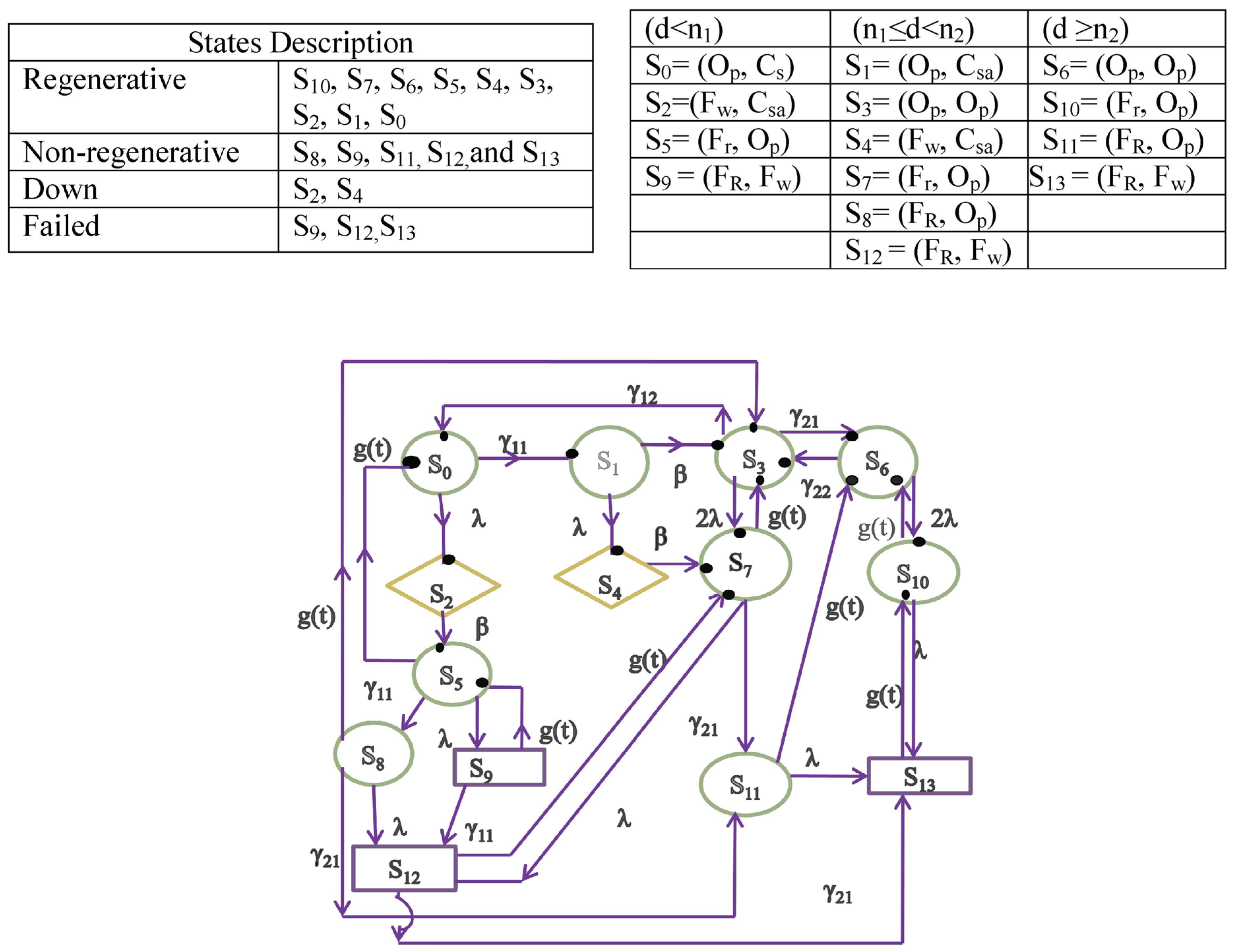
3. General Description of Model 1

Figure 1 depicts various possible transitions for Model 1 (a cold redundant system [36]). One operative and one redundant unit originally comprised a two-unit cold redundant system (state S₀). According to varying demand, the system is most certainly in one of the following states:

4. Measures of System Effectiveness of Model 1

Authors deal with the probabilities of transitioning between the states ‘i’ and ‘j’ and Mean sojourn times (µ_i) in state ‘i’.

4.1. Mean Sojourn Times and Transition Probabilities

Probabilities [36] describe the movement from one state to another in a single step and are given as follows:

$$q_{01}(t)={\gamma }_{11}{e}^{-\left({\gamma }_{11}+\lambda \right)t}$$

$$q_{02}\left(t\right)=\lambda e^{-\left({\gamma }_{11}+\lambda \right)t}$$

$$q_{13}\left(t\right)=\beta e^{-\left(\beta +\lambda \right)t}$$

$$q_{14}\left(t\right)=\lambda e^{-\left(\beta +\lambda \right)t}$$

$$q_{25}\left(t\right)=\beta e^{-\beta t}$$

Similarly, other probabilities of the given model respectively can be defined.

For the long run, non-zero steady-state probabilities p_ij are obtained as p_ij = $\underset{s\to 0}{\lim }$q_ij^∗(s) by simple probabilistic considerations and have been used to determine the steady-state availability analysis of a given model. Some of the values of the given model respectively are:

$$p_{01}=\frac{{\gamma }_{11}}{({\gamma }_{11}+\lambda )}$$

$$p_{02}=\frac{\lambda }{({\gamma }_{11}+\lambda )}$$

$$p_{13}=\frac{\beta }{(\beta +\lambda )}$$

$$p_{14}=\frac{\lambda }{(\beta +\lambda )}$$

$$p_{25}=1$$

The calculated probabilities follow the law of probability such as:

$$p_{01}+p_{02}=1$$

$$p_{13}+p_{14}=1$$

and so on. The mean sojourn times ${\mu }_i$ ${(\mu }_i)$ in a specific state ‘i’ is the total time a unit probably spends in a system before exiting it for betterment. ${\mu }_i$ in regenerative states ‘$S_i$’ (i = 10, 7, 6, 5, 4, 3, 2, 1, 0) are

$${\mu }_0=\frac{1}{{\lambda +\gamma }_{11}}$$

$${\mu }_1=\frac{1}{\lambda +\beta }$$

$${\mu }_2=\frac{1}{\beta }$$

$${\mu }_3=\frac{1}{{2\lambda +\gamma }_{21}{+\gamma }_{12}}$$

$${\mu }_4=\frac{1}{\beta }$$

$${\mu }_5=\frac{1-g^{\ast }\left({\lambda +\gamma }_{11}\right)}{{\lambda +\gamma }_{11}}$$

$${\mu }_6=\frac{1}{{2\lambda +\gamma }_{22}}$$

$${\mu }_7=\frac{1-g^{\ast }\left({\lambda +\gamma }_{21}\right)}{{\lambda +\gamma }_{21}}$$

$${\mu }_{10}=\frac{1-g^{\ast }\left(\lambda \right)}{\lambda }$$

The unconditional average engaged time, for instance, assesses how long users engage with the system and how effectively they can finish activities within a specific amount of time given by

$$m_{ij}={\int }_0^{\mathrm{\infty }}t{q}_{ij}\left(t\right)dt=-q_{ij}^{{\ast }^{\prime }}(0)$$

4.2. Mean Time to System Failure (MTSF)

Let the c.d.f of the initial transition be ϕ_i(t) (i = 10, 7, 6, 3, 1, 0). In this scenario, failed states are absorbing states. The likelihood of a system changing conditions over a predetermined time can be used to assess a system’s behavior. The projected total time till absorption is calculated by adding the predicted passage times for all possible state combinations.

$R\left(t\right)$ the reliability of the device is given by:

$$R\left(t\right)=\mathrm{Pr}\left[T>t\right]=1-\mathrm{Pr}\left[T\le t\right]=1-\varphi \left(t\right)$$

Take the Laplace transform (LT), $R^{\ast }\left(s\right)=\frac{1-{\varphi }^{\ast \ast }\left(s\right)}{s}$. Where $R^{\ast }\left(s\right)$ is LT of $R\left(t\right)$ and then take the limit

$$\underset{s\to 0}{\mathrm{MTSF}\left(\mathrm{M}1\right)=\lim }{R}^{\ast }\left(s\right)=\underset{S\to 0}{\lim }\frac{1-{\varphi }^{\ast \ast }\left(s\right)}{s}=\frac{\mathrm{N}}{\mathrm{D}}$$

$$\begin{gathered} N=\left({\mu }_0+{p_{01}\mu }_1\right)\left(\left(1-p_{\mathrm{6,10}}{p}_{\mathrm{10,6}}\right)\left(1-p_{37}{p}_{73}\right)-p_{63}{(p}_{36} \\ +p_{37}{p}_{76}^{11})\right)+p_{01}{p}_{13}\left({\mu }_3+{p_{37}\mu }_{10}\right)\left(1-p_{\mathrm{6,10}}{p}_{\mathrm{10,6}}\right) \\ +\left({\mu }_6+p_{\mathrm{6,10}}{\mu }_{10}\right)\left(\left(1+p_{01}{p}_{13}\right)({(p}_{36}+p_{37}{p}_{76}^{11})\right) \end{gathered}$$

$$D=\left(1-p_{\mathrm{6,10}}{p}_{\mathrm{10,6}}\right)\left(\left(1-p_{37}{p}_{73}-p_{01}{p}_{13}{p}_{30}\right)-p_{63}{(p}_{36}+p_{37}{p}_{76}^{11})\right)$$

4.3. Availability Analysis

The probability that the system is not presently experiencing a failure at a time “t” is known as availability “A(t).” It is true even if the system might have previously failed to resume normal operating conditions.

$$A_i(t)=M_i\left(t\right)+\sum _{\mathrm{j}}{q}_{i,j}^{\left(k\right)}(t)\copyright A_j(t),i\ne j$$

Assume that “t” is approaching infinite and “A” represents the limiting value of “A(t).”

The total availabilities identified in the following scenarios comprise the proposed system’s availability (A1): the operational divisions are one and two. Notably, there has yet to be any prior analysis of availability with variable demand in the literature.

Total availability [36] is the sum of all availabilities (when one unit is operational and two units are in operation) and is given by

Total availability (A1) in the steady-state is given by

$$A1=A_{01}^{n_{11}}+A_{01}^{n_{21}}+A_{01}^{d_1}+A_{01}^{n_{22}}+A_{01}^{d_2}$$

4.4. Busy Period Analysis of Repairman

Given that the system reached the state “Si” at t = 0 let B_i(t) (i = 0, 1, 2, 3, 4, 5, 6, 7, 10) be the probability that the repairman is working on a failed unit at any instant “t.” Recursive relations for B_i(t) are given by

$$B_i(t)=W_f\left(t\right)+{\sum }_{\mathrm{j}}{q}_{i,j}^{\left(k\right)}(t)\copyright B_j(t),i\ne j$$

W_f(t) (f = 7, 10) indicates the repairman is active in the ‘S_i’ state due to repair.

Take the Laplace transform of equations and solve for $B_0^{\ast }\left(s\right)$. Thus,

$$B_0=\underset{S\to 0}{lim}\left(s{B}_0^{\ast }\left(s\right)\right)=N_4/D_1$$

where

$$\begin{gathered} {N_4=k}_1|-p_{02}{p}_{25}((-p_{77}^{12})\left(p_{36}\left(1-p_{\mathrm{10,10}}^{13}\right)p_{63}-p_{\mathrm{6,10}}{p}_{\mathrm{10,6}} \\ +\left(1-p_{\mathrm{10,10}}^{13}\right)\right){+p}_{37}\left(p_{73}\left(p_{\mathrm{6,10}}{p}_{\mathrm{10,6}}-\left(1-p_{\mathrm{10,10}}^{13}\right)\right) \\ -p_{63}\left(p_{\mathrm{7,6}}^{11}\left(1-p_{\mathrm{10,10}}^{13}\right)+p_{\mathrm{10,6}}\left(p_{\mathrm{7,10}}^{\mathrm{11,13}}+p_{\mathrm{7,10}}^{\mathrm{12,13}}\right)\right)\right) \\ -\left[p_{01}(1-p_{55}^9)p_{13}{p}_{37}\left(p_{\mathrm{6,10}}{p}_{\mathrm{10,6}}-(1-p_{\mathrm{10,10}}^{13})\right) \\ +\left(p_{01}\left(1-p_{55}^9\right)p_{14}{p}_{47}+p_{02}{p}_{25}(p_{57}^{\mathrm{8,12}}+p_{57}^{\mathrm{9,12}})\right)\left(p_{\mathrm{6,10}}{p}_{\mathrm{10,6}}-\left(1-p_{\mathrm{10,10}}^{13}\right)(1 \\ -p_{36}{p}_{63})\right)+p_{37}(-p_{53}^8\left(p_{\mathrm{6,10}}{p}_{\mathrm{10,6}}-\left(1-p_{\mathrm{10,10}}^{13}\right)\right) \\ +p_{63}\left(\left(p_{\mathrm{5,10}}^{\mathrm{8,11,13}}+p_{\mathrm{5,10}}^{\mathrm{8,12,13}}+p_{\mathrm{5,10}}^{\mathrm{9,12,13}}\right)p_{\mathrm{10,6}}+\left(1-p_{\mathrm{10,10}}^{13}\right)p_{56}^{\mathrm{8,11}})\right)\right]+-p_{01}(1 \\ -p_{55}^9)(p_{36}{p}_{\mathrm{6,10}}\left(1-p_{77}^{12}\right)+p_{37}\left(\left(p_{\mathrm{7,10}}^{\mathrm{11,13}}+p_{\mathrm{7,10}}^{\mathrm{12,13}}\right)-p_{\mathrm{6,10}}{p}_{76}^{11}\right) \\ +p_{14}{p}_{47}\left(\left(-p_{36}{(p}_{\mathrm{6,10}}{p}_{73}-p_{63}\left(p_{\mathrm{7,10}}^{\mathrm{11,13}}+p_{\mathrm{7,10}}^{\mathrm{12,13}}\right)\right)-\left(p_{\mathrm{6,10}}{p}_{76}^{11}+\left(p_{\mathrm{7,10}}^{\mathrm{11,13}}+p_{\mathrm{7,10}}^{\mathrm{12,13}}\right)\right)\right) \\ +p_{02}{p}_{25}\left(p_{36}\left(p_{53}^8{p}_{\mathrm{6,10}}\left(1-p_{77}^{12}\right)+\left(p_{57}^{\mathrm{8,12}}+p_{57}^{\mathrm{9,12}}\right)\left(p_{73}{p}_{\mathrm{6,10}}-p_{63}\left(p_{\mathrm{7,10}}^{\mathrm{11,13}}+p_{\mathrm{7,10}}^{\mathrm{12,13}}\right)\right) \\ -\left(p_{\mathrm{5,10}}^{\mathrm{8,11,13}}+p_{\mathrm{5,10}}^{\mathrm{8,12,13}}+p_{\mathrm{5,10}}^{\mathrm{9,12,13}}\right)\left(1-p_{77}^{12}\right)p_{63}\right) \\ -p_{37}\left(-p_{53}^8\left(p_{\mathrm{6,10}}{p}_{76}^{11}+\left(p_{\mathrm{7,10}}^{\mathrm{11,13}}+p_{\mathrm{7,10}}^{\mathrm{12,13}}\right)\right)+p_{56}^{\mathrm{8,11}}\left(p_{\mathrm{6,10}}{p}_{73}-\left(p_{\mathrm{7,10}}^{\mathrm{11,13}}+p_{\mathrm{7,10}}^{\mathrm{12,13}}\right)p_{63}\right)\right) \\ +p_{56}^{\mathrm{8,11}}{p}_{\mathrm{6,10}}\left(1-p_{77}^{12}\right)-\left(p_{57}^{\mathrm{8,12}}+p_{57}^{\mathrm{9,12}}\right)\left(p_{\mathrm{6,10}}{p}_{76}^{11}+\left(p_{\mathrm{7,10}}^{\mathrm{11,13}}+p_{\mathrm{7,10}}^{\mathrm{12,13}}\right)\right) \\ +\left(1-p_{77}^{12}\right)\left(p_{\mathrm{5,10}}^{\mathrm{8,11,13}}+p_{\mathrm{5,10}}^{\mathrm{8,12,13}}+p_{\mathrm{5,10}}^{\mathrm{9,12,13}}\right)\right)| \end{gathered}$$

and D₁ is already defined.

4.5. Expected Number of Visits by Repairman

Let V_i (t) be the expected number of visits by the repairman in (0, t]. Recursive relations for V_i(t) are given by:

$$V_i\left(t\right)=\sum _{\mathrm{j}}{Q}_{i,j}^{\left(k\right)}\left(t\right)\mathrm{Ⓢ}\left)\right(V_j\left(t\right)+{\delta }_j\left(t\right))$$

“where ‘S_j’ is any regenerative state to which the regenerative state ‘S_i’ transits and  ${\delta }_j$ = 1 if ‘S_j’ is the regenerative state where the repairman does the job afresh, otherwise ${\delta }_j$ = 0. Taking the LST of equations and solving for V₀**(s) in the steady-state,” the expected number of visits is given by

$$V_0=\underset{S\to 0}{\lim }\left(s{V}_0^{\ast \ast }\left(s\right)\right)={\mathrm{N}}_5/{\mathrm{D}}_1$$

where

$$\begin{gathered} N_5=p_{02}{p}_{25}\left(\left(1-p_{55}^9\right)\right({-p}_{73}\left(p_{\mathrm{6,10}}{p}_{\mathrm{10,6}}-\left(1-p_{\mathrm{10,10}}^{13}\right)\right) \\ -p_{63}\left(p_{\mathrm{7,6}}^{11}\left(1-p_{\mathrm{10,10}}^{13}\right)+p_{\mathrm{10,6}}\left(p_{\mathrm{7,10}}^{\mathrm{11,13}}+p_{\mathrm{7,10}}^{\mathrm{12,13}}\right)\right)) \\ -p_{37}|-p_{01}\left(1-p_{55}^9\right)\left(-p_{13}\left(1-p_{77}^{12}\right)\left(p_{\mathrm{6,10}}{p}_{\mathrm{10,6}}-\left(1-p_{\mathrm{10,10}}^{13}\right)\right)\right) \\ +p_{14}{p}_{47}(-p_{73}\left(p_{\mathrm{6,10}}{p}_{\mathrm{10,6}}-\left(1-p_{\mathrm{10,10}}^{13}\right)\right) \\ +p_{63}\left(p_{\mathrm{7,6}}^{11}\left(1-p_{\mathrm{10,10}}^{13}\right)+p_{\mathrm{10,6}}\left(p_{\mathrm{7,10}}^{\mathrm{11,13}}+p_{\mathrm{7,10}}^{\mathrm{12,13}}\right)\right)) \\ +p_{02}{p}_{25}\left[\left(1-p_{77}^{12}\right)\right(p_{53}^8\left(p_{\mathrm{6,10}}{p}_{\mathrm{10,6}}-\left(1-p_{\mathrm{10,10}}^{13}\right)\right) \\ -p_{63}\left(p_{56}^{\mathrm{8,11}}\left(1-p_{\mathrm{10,10}}^{13}\right)+p_{\mathrm{10,6}}\left(p_{\mathrm{5,10}}^{\mathrm{8,11,13}}+p_{\mathrm{5,10}}^{\mathrm{8,12,13}}+p_{\mathrm{5,10}}^{\mathrm{9,12,13}}\right)\right)) \\ -\left(p_{57}^{\mathrm{8,12}}+p_{57}^{\mathrm{9,12}}\right)\left(-p_{73}\left(p_{\mathrm{6,10}}{p}_{\mathrm{10,6}}-\left(1-p_{\mathrm{10,10}}^{13}\right)\right) \\ +p_{63}\left(p_{\mathrm{7,6}}^{11}\left(1-p_{\mathrm{10,10}}^{13}\right)+p_{\mathrm{10,6}}\left(p_{\mathrm{7,10}}^{\mathrm{11,13}}+p_{\mathrm{7,10}}^{\mathrm{12,13}}\right)\right)\right)]| \\ +p_{\mathrm{6,10}}\left[-p_{01}\left(-p_{55}^9\right)\left(-p_{13}\left(-p_{36}\left(1-p_{77}^{12}\right)\left(1-p_{\mathrm{10,10}}^{13}\right) \\ -p_{37}\left(p_{\mathrm{10,6}}\left(p_{\mathrm{7,10}}^{\mathrm{11,13}}+p_{\mathrm{7,10}}^{\mathrm{12,13}}\right)+p_{\mathrm{7,6}}^{11}\left(1-p_{\mathrm{10,10}}^{13}\right)+p_{14}{p}_{47}\left(\right(p_{36}{p}_{73}-p_{76}^{11}\right)\left(1-p_{\mathrm{10,10}}^{13}\right) \\ +p_{\mathrm{10,6}}\left(p_{\mathrm{7,10}}^{\mathrm{11,13}}+p_{\mathrm{7,10}}^{\mathrm{12,13}}\right)\right)\right)-p_{02}{p}_{25}\left(p_{36}\left(1-p_{\mathrm{10,10}}^{13}\right)\right(-p_{53}^8\left(1-p_{77}^{12}\right) \\ -p_{73}\left(p_{57}^{\mathrm{8,12}}+p_{57}^{\mathrm{9,12}}\right) \\ -p_{37}(-p_{53}^8\left(-p_{\mathrm{7,6}}^{11}\left(1-p_{\mathrm{10,10}}^{13}\right)+p_{\mathrm{10,6}}\left(p_{\mathrm{7,10}}^{\mathrm{11,13}}+p_{\mathrm{7,10}}^{\mathrm{12,13}}\right))+p_{73}\left({-p}_{56}^{\mathrm{8,11}}\left(1-p_{\mathrm{10,10}}^{13}\right)\right) \\ -p_{\mathrm{10,6}}\left(p_{\mathrm{5,10}}^{\mathrm{8,11,13}}+p_{\mathrm{5,10}}^{\mathrm{8,12,13}}+p_{\mathrm{5,10}}^{\mathrm{9,12,13}}\right)))-p_{56}^{\mathrm{8,11}}\left(1-p_{77}^{12}\right)\left(1-p_{\mathrm{10,10}}^{13}\right) \\ +\left(p_{57}^{\mathrm{8,12}}+p_{57}^{\mathrm{9,12}}\right)\left(-p_{\mathrm{7,6}}^{11}\left(1-p_{\mathrm{10,10}}^{13}\right)-p_{\mathrm{10,6}}\left(p_{\mathrm{7,10}}^{\mathrm{11,13}}+p_{\mathrm{7,10}}^{\mathrm{12,13}}\right)\right) \\ -\left(1-p_{77}^{12}\right)p_{\mathrm{10,6}}\left(p_{\mathrm{5,10}}^{\mathrm{8,11,13}}+p_{\mathrm{5,10}}^{\mathrm{8,12,13}}+p_{\mathrm{5,10}}^{\mathrm{9,12,13}}\right)\right)\right] \end{gathered}$$

and D₁ is already defined.

4.6. Expected Activation Time of Unit

Let AT_i (t) be the expected activation time. Recursive relations for AT_i(t) are given by

$${AT}_i(t)=W_f\left(t\right)+\sum _{\mathrm{j}}{q}_{i,j}^{\left(k\right)}(t)\copyright {AT}_j(t),i\ne j$$

where W_f(t) (f = 1, 2, 4) = $e^{-\mathsf{\beta }\mathrm{t}}$.

Take the Laplace transform of equations given above and solve,

In the steadystate, the expected activation time of the standby unit in cold standby is given by:

AT₀ = N₆/D₁

where

And D₁ is already defined.

$$\begin{gathered} N_6={\mu }_2{p}_{02}(\left(1-p_{55}^9\right)\left(p_{37}{-p}_{73}\left(p_{\mathrm{6,10}}{p}_{\mathrm{10,6}}-\left(1-p_{\mathrm{10,10}}^{13}\right)\right) \\ -p_{63}\left(p_{\mathrm{7,6}}^{11}\right)+{\left(p_{\mathrm{7,10}}^{\mathrm{11,13}}+p_{\mathrm{7,10}}^{\mathrm{12,13}}\right)}_{}\right) \\ -\left(\left(1-p_{77}^{12}\right)\left(p_{36}\left(1-p_{\mathrm{10,10}}^{13}\right)p_{63}+p_{\mathrm{6,10}}{p}_{\mathrm{10,6}} \\ -\left(1-p_{\mathrm{10,10}}^{13}\right)\right)\right) \\ +\left(p_{01}(\left(1-p_{55}^9\right)\left({\mu }_1+p_{14}{\mu }_4\right)\right)(1 \\ -p_{77}^{12}\left)\right(p_{36}{\left(1-p_{\mathrm{10,10}}^{13}\right)p}_{63}-p_{\mathrm{6,10}}{p}_{\mathrm{10,6}} \\ +\left(1-p_{\mathrm{10,10}}^{13}\right)) \\ +p_{37}\left(p_{73}\left(p_{\mathrm{6,10}}{p}_{\mathrm{10,6}}-\left(1-p_{\mathrm{10,10}}^{13}\right)\right) \\ -p_{63}\left(p_{\mathrm{7,6}}^{11}\left(1-p_{\mathrm{10,10}}^{13}\right)+p_{\mathrm{10,6}}\left(p_{\mathrm{7,10}}^{\mathrm{11,13}}+p_{\mathrm{7,10}}^{\mathrm{12,13}}\right)\right)\right) \end{gathered}$$

4.7. Profit Analysis

In a steady-state, profit is given by the sum of individual expected profits in two cases,

i.e., P1 = P11 + P12

where, $Profit(P11)=C_0{A}_0^{n_{11}}+{C_{1}A}_0^{n_{21}}+{C_{2}A}_0^{d_1}-C_3{B}_0-C_4{V}_1-C_5{AT}_0$

$$\mathrm{P}\mathrm{r}\mathrm{o}\mathrm{f}\mathrm{i}\mathrm{t}(P12)=C_1{A}_0^{n_{22}}+{C_{2}A}_0^{d_2}-C_3{B}_0-C_4{V}_1-C_5{AT}_0$$

P11 and P12 specify the profits in model 1 when a single unit or two units are operative.

5. Proposed System (Model 2)

Figure 2 depicts the feasible states of Model 2 (a two-unit hot redundant system). One unit is operational at startup (state S₀), and the other is on hot standby (fully loaded). The redundant unit is susceptible to failure because it is always operational. Nonetheless, the hot standby failure rate is expected to be lower than the active unit failure rates. The system enters the state S₁ if demand rises (where the need is greater or equal to the order produced by one unit but less than that produced by two units). The system enters the state S₅ in response to further increases in demand. In a different scenario, the system switches to state S₂ if a unit fails. If the unit is fixed, another unit fails, or the demand increases, it returns to state S₀, state S₃, or state S₄. The system moves to state S₉ and then to S₁₀ in the event of greater demand. The system may switch from S₅ to S₁ or S₇, depending on the situation. Depending on variation in need, the system may be in one of the following states.

Model 2’s transition and steady-state probabilities, availabilities, and steady-state measures of system effectiveness, including MTSF, have been calculated similarly for Model 1 (in Section 5).

Transition Probabilities and Mean Sojourn Times of Model 2

Probabilities (transition) are time-dependent and describe the movement from one state to another in a single step. These probabilities are given as follows:

$$q_{01}\left(t\right)={\gamma }_{11}{e}^{-\left({\gamma }_{11}+\lambda +{\lambda }_1\right)t}$$

$$q_{02}\left(t\right)=(\lambda +{\lambda }_1)e^{-\left({\gamma }_{11}+\lambda +{\lambda }_1\right)t}$$

$$q_{10}\left(t\right)={\gamma }_{12}{e}^{-\left({\gamma }_{12}+{\gamma }_{21}+\lambda +{\lambda }_1\right)t}$$

$$q_{15}\left(t\right)={\gamma }_{21}{e}^{-\left({\gamma }_{12}+{\gamma }_{21}+\lambda +{\lambda }_1\right)t}$$

$$q_{16}\left(t\right)=(\lambda +{\lambda }_{21})e^{-\left({\gamma }_{12}+{\gamma }_{21}+\lambda +{\lambda }_1\right)t}$$

For the long run, non-zero steady-state probabilities p_ij are obtained as p_ij = $\underset{s\to 0}{\lim }$q_ij^∗(s) by simple probabilistic considerations. Some of the values of the given model respectively are:

$$p_{01}=\frac{{\gamma }_{11}}{{\lambda +{\lambda }_1+\gamma }_{11}}$$

$$p_{02}=\frac{\lambda +{\lambda }_1}{{\lambda +{\lambda }_1+\gamma }_{11}}$$

$$p_{10}=\frac{{\gamma }_{12}}{{\lambda +{\lambda }_1+{\gamma }_{21}+\gamma }_{12}}$$

$$p_{15}=\frac{{\gamma }_{21}}{{\lambda +{\lambda }_1+{\gamma }_{21}+\gamma }_{12}}$$

$$p_{16}=\frac{\lambda +{\lambda }_1}{{\lambda +{\lambda }_1+{\gamma }_{21}+\gamma }_{12}}$$

Similarly, other probabilities of the given model respectively can be defined.

The mean sojourn time (µ_i) in the state ‘i’ are

$${\mu }_0=\frac{1}{\lambda +{\lambda }_1+{\gamma }_{11}}$$

$${\mu }_1=\frac{1}{{\lambda +{\lambda }_1+{\gamma }_{21}+\gamma }_{12}}$$

$${\mu }_2=\frac{1-{\mathrm{g}}^{\mathrm{*}}(\lambda +{\gamma }_{11})}{\lambda +{\gamma }_{11}}$$

$${\mu }_5=\frac{1}{\lambda +{\lambda }_1+{\gamma }_{22}}$$

$${\mu }_6=\frac{1-{\mathrm{g}}^{\mathrm{*}}(\lambda +{\gamma }_{21})}{\lambda +{\gamma }_{21}}$$

$${\mu }_6=\frac{1-{\mathrm{g}}^{\mathrm{*}}\left(\lambda \right)}{\lambda }$$

For Model 2, other measures of system effectiveness, including MTSF, have been calculated similarly to what was done for Model 1 (in Section 5). Based on variation in demand, three sub-cases (n₁ ≤ d < n₂), (d < n₁), and (d ≥ n₂) are identified. The solution of the proposed SMP (Model 2) based on the same approach outlined earlier yields the total availability (A2) in the steady-state, busy period (B₂), and visiting time of the repairman (V₂). Similarly, the profit (P2) is given by

P2 = P21 + P22

where, $Profit(P21)=C_0{A}_0^{n_{11}}+{C_{1}A}_0^{n_{21}}+{C_{2}A}_0^{d_1}-C_3{B}_0-C_4{V}_0$

$$Profit(P22)=C_1{A}_0^{n_{12}}+C_1{A}_0^{n_{22}}+{C_{2}A}_0^{d_2}-C_3{B}_0-C_4{V}_0$$

where the symbols have their usual meanings.

6. Comparative Analysis

Each model has strengths and weaknesses; therefore, no single model suits every situation. Hence, it becomes essential to undertake a comparative study to decide the type of standby (Model 1 and Model 2) used for the systems with varying demands.

Authors have studied (Figure 3, Figure 4, Figure 5, Figure 6, Figure 7 and Figure 8) MTSF, steady-state availability, and profit. Take g(t) = α e^−αt, where α is the repair rate. Let C₀ = 6000, C₁ = 4500, C₂ = 1200, C₃ = 600, C₄ = 800, C₅ = I400, α = 0.05, γ₁₂ = 0.07, γ₁₁ = 0.235, γ₂₁ = 0.4213, γ₂₂ = 0.3153, λ₁ = 0.0013, β = 0.00351, andλ = 0.003. Various graphs (Figure 3, Figure 4, Figure 5, Figure 6, Figure 7 and Figure 8) are plotted to find cut-off points for different parameters revealing the betterment of one model over the other. The interpretations are discussed below.

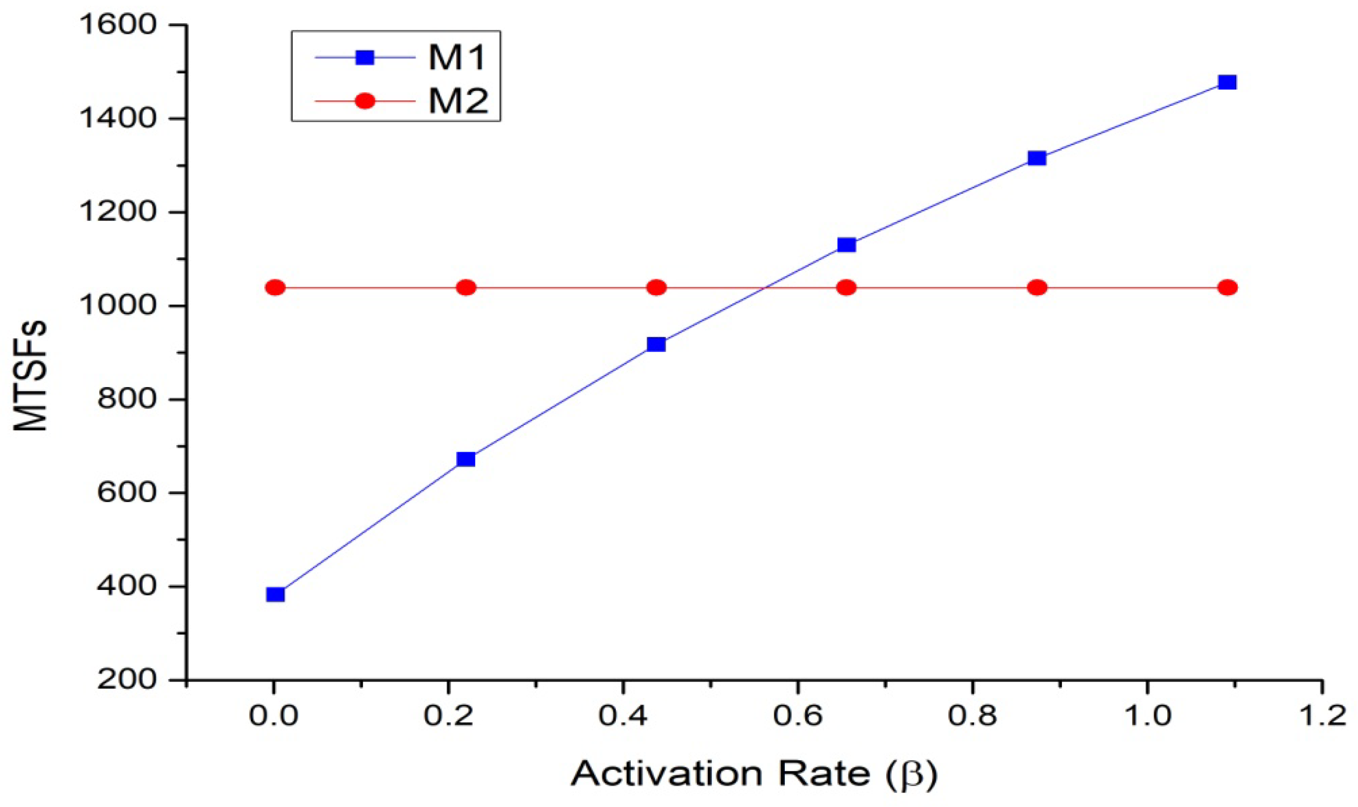
Figure 3 and Figure 4 show the MTSFs (M2, M1) of Model 2 and Model 1 about the activation rate (β) and failure rate (λ₁). It shows that as β> or = or < 0.548, M1 > or = < M2 accordingly. Thus, for β > 0.548, the cold standby system exhibits better results than the hot standby system.

Figure 3. Variation of MTSFs (M1, M2) about the activation rate (β).

Figure 3. Variation of MTSFs (M1, M2) about the activation rate (β).

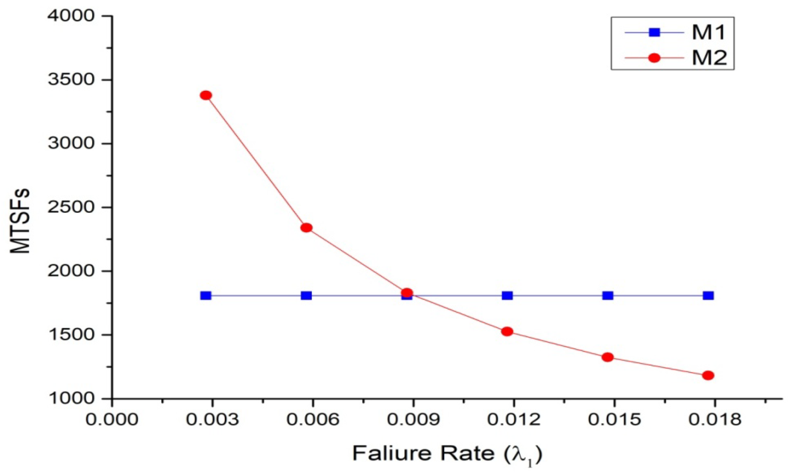
Figure 4 depicts that M2 decreases as λ₁ increases, but M1 remains the same. Further, M1 is < or = > M2 according to λ₁ < or = or > 0.0098. Thus, for λ₁ < 0.0098, the hot standby system is superior to the cold one.

Figure 4. Variation of MTSFs (M1, M2) about the failure rate (λ₁).

Figure 4. Variation of MTSFs (M1, M2) about the failure rate (λ₁).

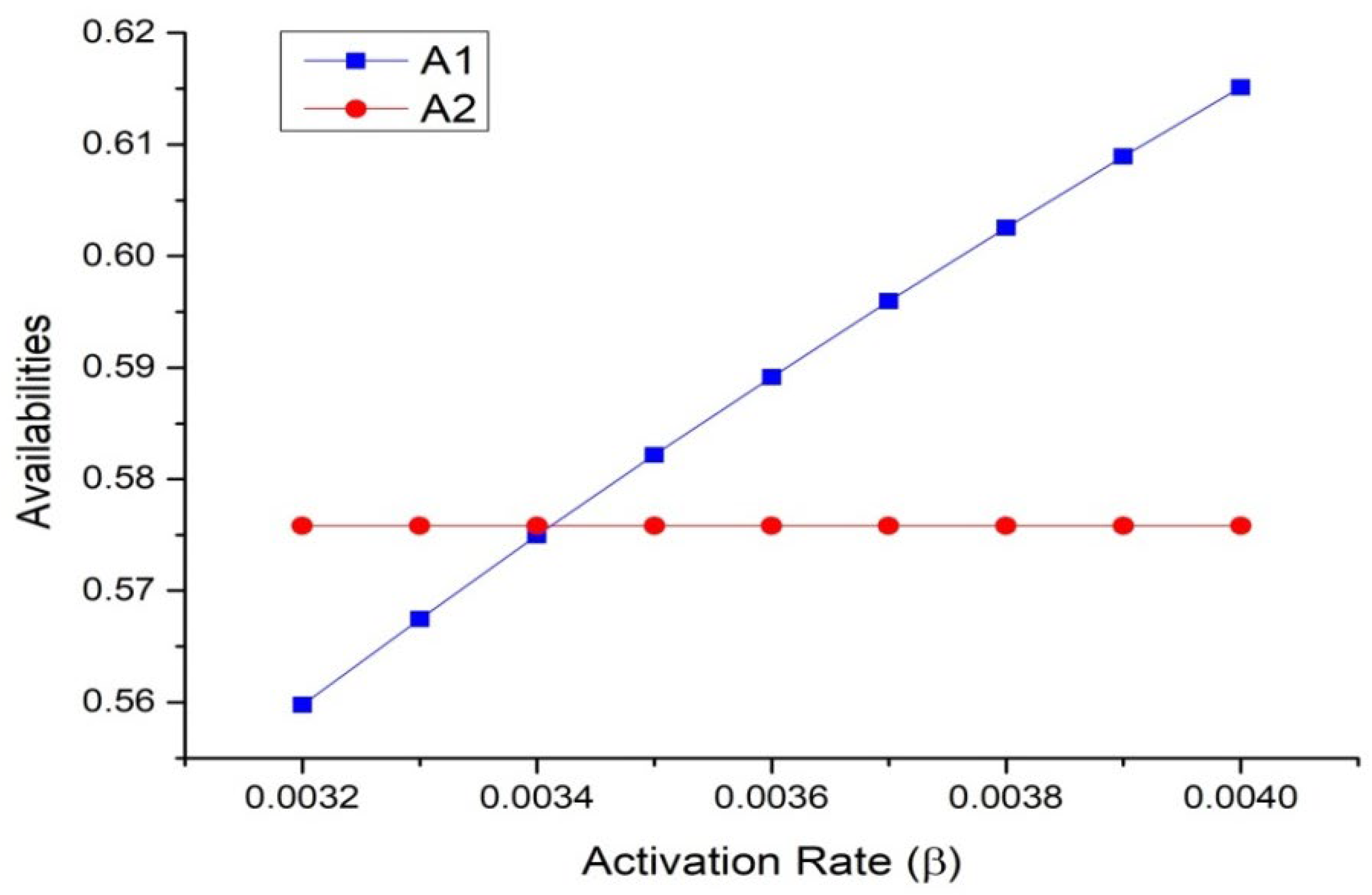
Figure 5 exhibits the variation of availability (A1/A2) about λ₁. Notice that A1 > or = or < A2 as β > or = or < 0.00343. Thus, for β > 0.00343, a cold standby system is preferred over a hot one.

Figure 5. Variation of availability (A1/A2) about the activation rate (β).

Figure 5. Variation of availability (A1/A2) about the activation rate (β).

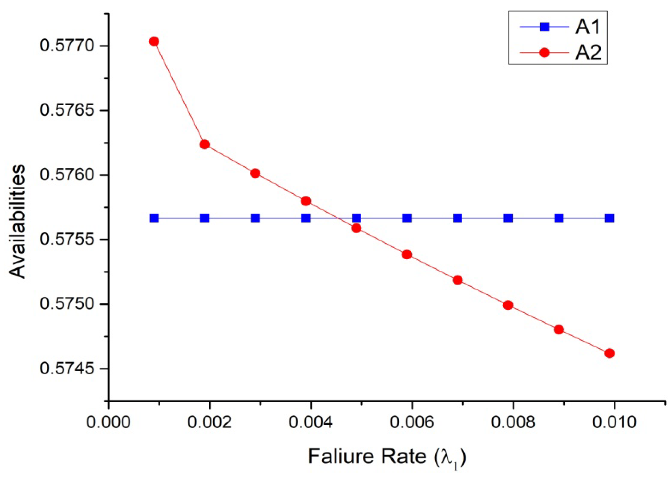
Figure 6 reveals the variation of availability (A1/A2) about the failure rate of the hot standby unit (λ₁). A2 > or = A1 as λ₁ < or = or > 0.00395. Thus, for λ₁< 0.00395, a hot standby system is preferred over a cold one.

Figure 6. Variation of availability (A1/A2) about the failure rate (λ₁).

Figure 6. Variation of availability (A1/A2) about the failure rate (λ₁).

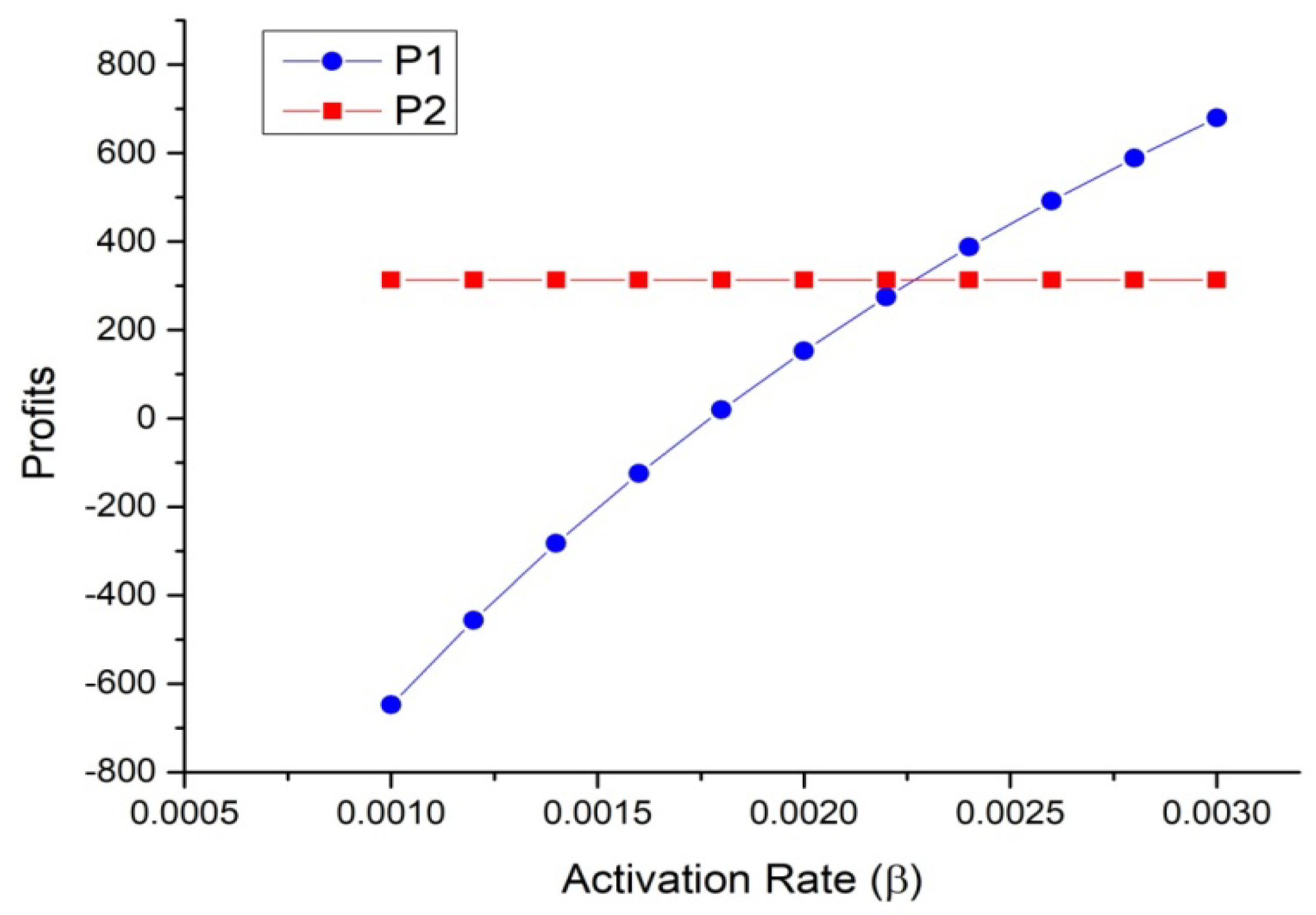
Figure 7 depicts the variation of profits (P1, P2) about the activation rate (β). The graph concludes that with the increase in β, P1 increases, whereas P2 remains unaffected. Notice that P1 > or = or < P2 as β > or = or < 0.0023.

Figure 7. Variation of profits (P1, P2) in reference to the activation rate (β).

Figure 7. Variation of profits (P1, P2) in reference to the activation rate (β).

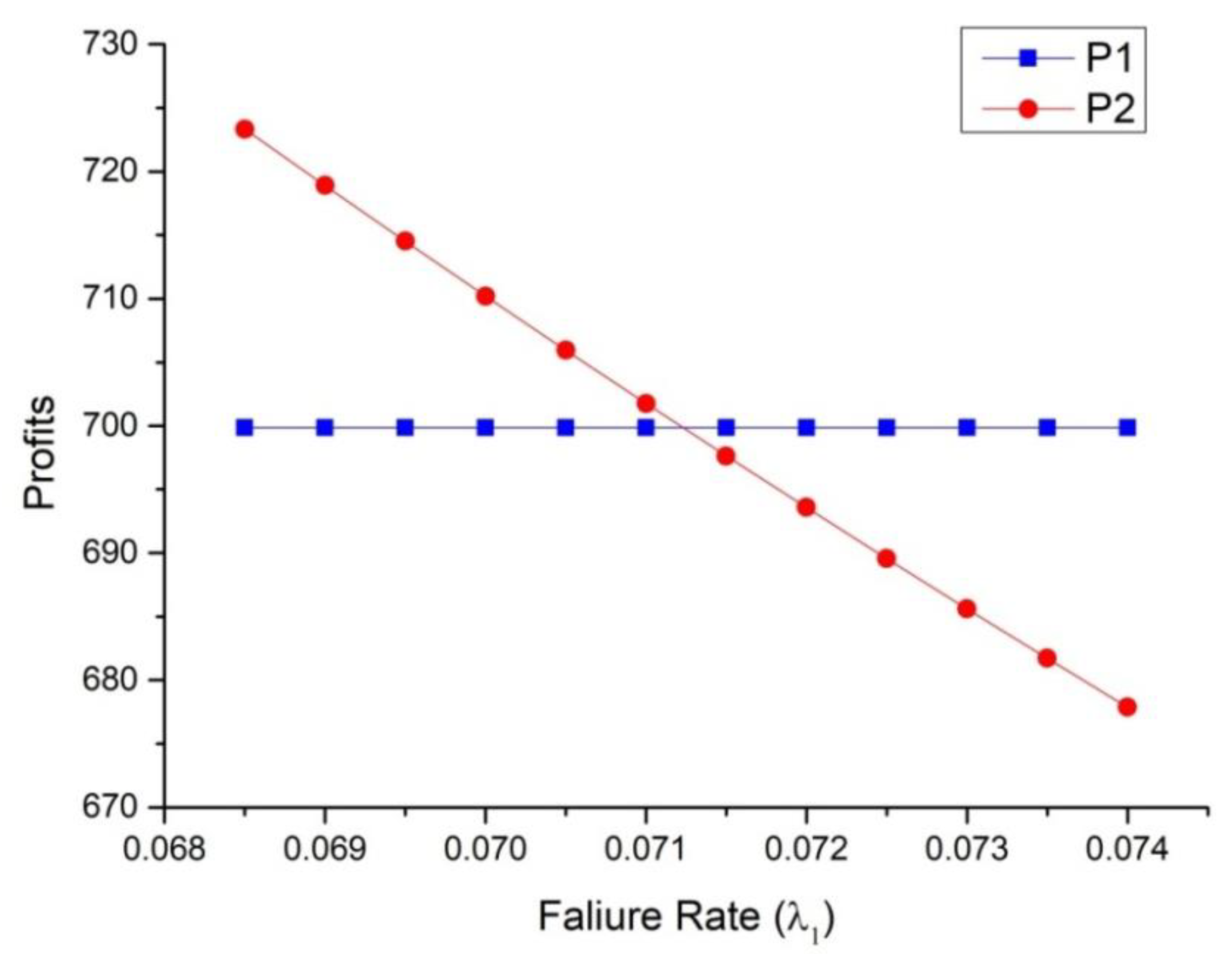
Figure 8 illustrates that when λ₁ increases, P2 decreases, but P1 remains unaffected. Further, a hot standby system is costlier than a cold standby system if λ₁ > 0.07056 or demand remains less most of the time.

Figure 8. Variation of profits (P1, P2) about the failure rate (λ₁).

Figure 8. Variation of profits (P1, P2) about the failure rate (λ₁).

Cut-off points observed from the graphs are given in

Table 1. Cut-off points regarding adoptability of one model over other.

Measure	Decision
	A Cold Standby System Is Superior If	A Hot StandbySystem Is Superior If	Both sTandby Systems Are Equally Superior
MTSFs (M1,M2)	β > 0.548	β < 0.548	β = 0.548
	λ1 > 0.0098	λ1 < 0.0098	λ1 = 0.0098
Total Availabilities (A1,A2)	β > 0.00343	β < 0.00343	β = 0.00343
	λ1 > 0.00395	λ1 < 0.00395	λ1 = 0.00395
Profits(P1, P2)	β > 0.0023	β < 0.0023	β = 0.0023
	λ1 > 0.07056	λ1 < 0.07056	λ1 = 0.07056

as follows:

7. Conclusions

The paper compares two-unit hot and cold standby systems with varied demand using the semi-Markov process and regenerative point technique symmetrically. The authors observed the situation existing in cable manufacturing plants. In cold standby, MTSF, profit, and availability improve with greater activation rate values (β), but in hot standby, these metrics rise with lower failure rate values (λ₁). The study suggests the system analyst hot standby system is more expensive than the cold standby system under three circumstances: either there is a decrease in demand, the hot standby unit’s failure rate exceeds a predetermined threshold, or the cold standby system’s activation time does not exceed a certain point, and it becomes necessary to turn both units on at once to handle the increasing demand. These general models may be used by any company where such situations exist. The users of such systems may observe the impact on the efficacy measures concerning the parameters of interest according to their needs and based on the data at their disposal and then make significant inferences regarding the system’s profitability.

References

- Balagurusamy, E. Reliability Engineering; Tata Mc Graw Hill Publishing Company Ltd.: New Delhi, India, 1984. [Google Scholar]
- Kuo, W.; Prasad, V.R.; Tillman, F.A.; Hwang, C.L. Optimal Reliability Design: Fundamentals and Applications; Cambridge University Press: Cambridge, UK, 2001. [Google Scholar]
- Elerath, J.G.; Pecht, M. A highly accurate method for assessing the reliability of redundant arrays of inexpensive disks (raid). IEEE Trans. Comput. 2009, 58, 289–299. [Google Scholar] [CrossRef]
- Hsieh, C.; Hsieh, Y. Reliability and cost optimization in distributed computing systems. Comput. Oper. Res. 2003, 30, 1103–1119. [Google Scholar] [CrossRef]
- Malhotra, R.; Taneja, G. Comparative Analysis of Two Stochastic Models with Varying Demand. Int. J. Appl. Eng. 2015, 10, 37453–37460. [Google Scholar]
- Ng, Y.W.; Avizienis, A.A. A unified reliability model for fault-tolerant computers. IEEE Trans. Comput. 1980, 29, 1002–1011. [Google Scholar]
- Amari, S.V.; Xing, L.; Shrestha, A.; Akers, J.; Trivedi, K.S. Performability analysis of multi-state computing systems using multivalued decision diagrams. IEEE Trans. Comput. 2010, 59, 1419–1433. [Google Scholar] [CrossRef]
- Malhotra, R. Reliability evaluation with variation in demand. In Systems Reliability Engineering: Modeling and Performance Improvement; Kumar, A., Ram, M., Eds.; De Gruyter: Berlin, Germany, 2021; pp. 89–100. [Google Scholar] [CrossRef]
- Sultan, K.S.; Moshref, M.E. Stochastic analysis of a priority standby system under preventive maintenance. Appl. Sci. 2021, 11, 3861. [Google Scholar] [CrossRef]
- Houankpo, H.G.K.; Kozyrev, D. Mathematical and Simulation Model for Reliability Analysis of a Heterogeneous Redundant Data Transmission System. Mathematics 2021, 9, 2884. [Google Scholar] [CrossRef]
- Taneja, G.; Naveen, V. Comparative study of two reliability models with patience time and chances of non-availability of expert repairman. Pure Appl. Math. Sci. 2003, LVII, 23–35. [Google Scholar]
- Wang, K.H.; Ke, J.C. Probabilistic analysis of a repairable system with warm standbys plus balking and reneging. Appl. Math. Model. 2003, 27, 327–336. [Google Scholar] [CrossRef]
- Zhao, R.; Liu, B. Standby redundancy optimization problems with fuzzy lifetimes. Comput. Ind. Eng. 2005, 49, 318–338. [Google Scholar] [CrossRef]
- Khurana, V.; Rizwan, S.M.; Taneja, G. Economics analysis of reliability model for two PLC cold standby system with four types of failures. Pure Appl. Math. Sci. 2006, 63, 65–78. [Google Scholar]
- Wang, K.H.; Ke, J.B.; Lee, W.C. Reliability and sensitivity analysis of a repairable system with warm standbys and R unreliable service station. Int. J. Adv. Manuf. Technol. 2007, 31, 1223–1232. [Google Scholar] [CrossRef]
- Parashar, B.; Taneja, G. Reliability and profit evaluation of a PLC hot standby system based on a master-slave concept and two types of repair facilities. IEEE Trans. Reliab. 2007, 56, 534–539. [Google Scholar] [CrossRef]
- Rizwan, S.M.; Khurana, V.; Taneja, G. Reliability analysis of a hot standby industrial system. Int. J. Model. Simul. 2010, 30, 315–322. [Google Scholar] [CrossRef]
- Nakagawa, T. On a replacement problem of a cumulative damage model. J. Oper. Res. Soc. 1976, 27, 895–900. [Google Scholar] [CrossRef]
- Leung, K.F.; Zhang, Y.L.; Lai, K.K. Analysis for a two-dissimilar-component cold standby repairable system with repair priority. Reliab.Eng. Syst. Saf. 2011, 96, 1542–1551. [Google Scholar] [CrossRef]
- Batra, S.; Malhotra, R. Reliability and Availability Analysis of a Standby System of PCB Manufacturing Unit. In Reliability and Risk Modeling of Engineering Systems. EAI/Springer Innovations in Communication and Computing; Panchal, D., Chatterjee, P., Pamucar, D., Tyagi, M., Eds.; Springer: Cham, Switzerland, 2021. [Google Scholar] [CrossRef]
- Barron, Y.; Frostig, E.; Levikson, B. Analysis of R-out-of-N repairable systems: The case of phase-type distributions. Adv. Appl. Probab. 2004, 36, 116–138. [Google Scholar] [CrossRef]
- Malhotra, R.; Taneja, G. Stochastic analysis of a two-unit cold standby system wherein both the units may become operative depending upon the demand. J. Qual. Reliab. Eng. 2014, 13, 896379. [Google Scholar] [CrossRef]
- Malhotra, R.; Taneja, G. Comparative study between a single unit system and a two-unit cold standby system with varying demand. Springerplus 2015, 4, 705. [Google Scholar] [CrossRef]
- Levitin, G.; Xing, L.; Dai, Y. Cold vs. hot standby mission operation cost minimization for 1-out-of-N systems. Eur. J. Oper. Res. 2014, 234, 155–162. [Google Scholar] [CrossRef]
- Levitin, G.; Xing, L.; Dai, Y. Cold standby systems with imperfect backup. IEEE Trans. Reliab. 2016, 65, 1798–1809. [Google Scholar] [CrossRef]
- Garg, H. Multi-objective optimization problem of system reliability under intuitionistic fuzzy set environment using Cuckoo search algorithm. J. Intell. Fuzzy Syst. 2015, 29, 1653–1669. [Google Scholar] [CrossRef]
- Jiang, T.; Liu, Y. Parameter inference for non-repairable multi-state system reliability models by multi-level observation sequences. Reliab. Eng. Syst. Safety 2017, 166, 3–15. [Google Scholar] [CrossRef]
- Malhotra, R.; Dureja, T.; Goyal, A. Reliability Analysis a Two-Unit Cold Redundant System Working in a Pharmaceutical Agency with the Preventive Maintenance. In Journal of Physics: Conference Series; IOP Publishing: Bristol, UK, 2021; Volume 1850, p. 12087. [Google Scholar]
- Mantri, A.; Dutt, S.; Gupta, J.P.; Chitkara, M. Design and Evaluation of a PBL-Based Course in Analog Electronics. IEEE Trans. Educ. 2008, 51, 432–438. [Google Scholar] [CrossRef]
- Lilhore, U.K.; Poongodi, M.; Kaur, A.; Simaiya, S.; Algarni, A.D.; Elmannai, H.; Vijayakumar, V.; Tunze, G.B.; Hamdi, M. Hybrid Model for Detection of Cervical Cancer Using Causal Analysis and Machine Learning Techniques. Comput. Math. Methods Med. 2022, 2022, 132–148. [Google Scholar] [CrossRef]
- Liang, Z.; Parlikad, A.K. Predictive group maintenance for multi-system multicomponent networks. Reliab. Eng. Syst. Saf. 2020, 195, 106704. [Google Scholar] [CrossRef]
- Dong, F.; Gao, J.; Hao, A.; Wei, Y.; Huang, X.; Shi, F.; Zheng, K. A New Approach to Symmetry Reliability: Combination of Forward and Inverse Reliability Principle and Its Application to Frame Structures and Bamboo Bridges. Symmetry 2022, 14, 318. [Google Scholar] [CrossRef]
- Gao, S.; Wang, J. Reliability and availability analysis of a retrial system with mixed standbys and an unreliable repair facility. Reliab. Eng. Syst. Saf. 2021, 205, 107240. [Google Scholar] [CrossRef]
- Jiao, L.; Yan, R. Stochastic Comparisons of Lifetimes of Series and Parallel Systems with Dependent Heterogeneous MOTL-G Components under Random Shocks. Symmetry 2021, 13, 2248. [Google Scholar] [CrossRef]
- Ahmed, H.M.; El-Borai, M.M.; El-Sayed, W.G.; Elbadrawi, A.Y. Fractional Stochastic Evolution Inclusions with Control on the Boundary. Symmetry 2023, 15, 928. [Google Scholar] [CrossRef]
- Malhotra, R. Reliability and Availability Analysis of a Standby System with Activation time and varied demand. In Engineering Reliability and Risk Assessment; Elsevier: Amsterdam, The Netherlands, 2023; pp. 35–51. [Google Scholar] [CrossRef]
Figure 1.
Schematic of state transition for Model 1 (backup unit requires some activation time to begin functioning).
Figure 2.
Schematic of state transition diagram of Model 2.