An Improved Two-Stage Spherical Harmonic ESPRIT-Type Algorithm

Abstract

Sensor arrays are gradually becoming a current research hotspot due to their flexible beam control, high signal gain, robustness against extreme interference, and high spatial resolution. Among them, spherical microphone arrays with complex rotational symmetry can capture more sound field information than planar arrays and can convert the collected multiple speech signals into the spherical harmonic domain for processing through spherical modal decomposition. The subspace class direction of arrival (DOA) estimation algorithm is sensitive to noise and reverberation, and its performance can be improved by introducing relative sound pressure and frequency-smoothing techniques. The introduction of the relative sound pressure can increase the difference between the eigenvalues corresponding to the signal subspace and the noise subspace, which is helpful to estimate the number of active sound sources. The eigenbeam estimation of signal parameters via the rotational invariance technique (EB-ESPRIT) is a well-known subspace-based algorithm for a spherical microphone array. The EB-ESPRIT cannot estimate the DOA when the elevation angle approaches 90°. Huang et al. proposed a two-step ESPRIT (TS-ESPRIT) algorithm to solve this problem. The TS-ESPRIT algorithm estimates the elevation and azimuth angles of the signal independently, so there is a problem with DOA parameter pairing. In this paper, the DOA parameter pairing problem of the TS-ESPRIT algorithm is solved by introducing generalized eigenvalue decomposition without increasing the computation of the algorithm. At the same time, the estimation of the elevation angle is given by the arctan function, which increases the estimation accuracy of the elevation angle of the algorithm. The robustness of the algorithm in a noisy environment is also enhanced by introducing the relative sound pressure into the algorithm. Finally, the simulation and field-testing results show that the proposed method not only solves the problem of DOA parameter pairing, but also outperforms the traditional methods in DOA estimation accuracy.

1. Introduction

Multisource DOA estimation based on microphone arrays is a current research hotspot [1], and the estimation results are a priori knowledge for many acoustic applications such as speech separation [2], speech enhancement [3], and multisource localization [4]. A spherical microphone array has a three-dimensional symmetric structure, which allows us to estimate the orientation of a sound source at any position in three-dimensional space [5]. The spherical microphone array enables sampling of non-confounding sound pressure to reconstruct the 3D sound field accurately. The sound pressure received by the spherical microphone array can be easily decomposed into the spherical harmonic domain for processing [6]. The frequency and angular components of the spherical harmonic signal obtained through spherical harmonic decomposition are decoupled from each other, which is a major advantage of using the spherical harmonic domain as the space domain. Therefore, in recent years, sound source localization based on the spherical microphone array has received great attention.

Traditional DOA estimation methods mainly include: the spatial spectrum estimation algorithm based on conventional beamforming (CBF) [7]; the Capon method, also known as the minimum variance distortion response (MVDR) algorithm or the minimum variance method (MVM) [8]; the DOA estimation method based on TDOA [9]; the DOA estimation method based on steered-response power-phase transform [10]; etc. Traditional DOA estimation methods cannot break through the Rayleigh limit (Fourier limit). Subspace algorithms represented by the MUSIC algorithm and ESPRIT algorithm [11,12,13,14,15,16,17] have been proposed to solve this problem. Therefore, subspace algorithms are receiving great attention. However, such methods are sensitive to noise and reverberation and have large calculations. These disadvantages have a great impact on the practical applications of the algorithms and are worth in-depth consideration.

Due to the advantages of processing in the spherical harmonic domain, many DOA estimation techniques are being revisited in the spherical harmonic domain. For example, the steered-response power method manipulates the beamformer on the grid and checks the peak power output as an estimate of the DOA. In the simplest situations, a plane-wave decomposition (PWD) beamformer can be steered in multiple directions on a grid, forming a power map. Then, the peak finding on the map can be used to determine potential source DOAs. The spatial resolution of this approach is limited by the available order of the SH signals, and for low orders, the resolution is poor [18]. Similar to PWD estimation, the power map is formed with an MVDR beamformer. Because the signals’ statistics are considered in this case, the spatial resolution can be significantly higher [8]. Another alternative is to utilize the acoustic intensity vector obtained from the first-order signals, whose temporal and spatial statistics reveal information about the presence and distribution of the sound sources [19]. There are more approaches, such as the sparse recovery approach [20], the GCC (generalized cross-correlation) technique [21], and the adaptive eigenvalue decomposition method [22]. In addition, subspace algorithms have received increasing attention due to their high resolution and noise suppression capabilities [23]. Examples include the eigenbeam multiple signal classification (EB-MUSIC) [8,11] algorithms, which exploit the orthogonality between signal and noise subspaces, and the eigenbeam estimation algorithms for signal parameters via the rotational invariance technique (EB-ESPRIT), which exploit the rotation invariance properties of subsets of array channels [12]. Among these methods, EB-ESPRIT approaches estimate DOA parameters directly using the recurrence relations of spherical harmonic functions without beam steering or a peak search, which makes them well suited for real-time speech applications. Despite these advantages, EB-ESPRIT algorithms fail when the elevation angle approaches $90^{\circ }$. The abovementioned subspace algorithms, including the EB-ESPRIT algorithms, also require a priori knowledge about the number of active sound sources.

Many attempts have been made to resolve the singularity problem of EB-ESPRIT. Sun et al. [12] proposed a robust sound source localization method that rotates the eigenbeam space using a Wigner-D weighting matrix. However, the method requires a priori knowledge of the region of interest to guide the rotation. Huang et al. [13] proposed a two-step EB-ESPRIT algorithm (TS-ESPRIT), which uses different recurrence relations to estimate the elevation and azimuth angles separately. However, the elevation and azimuth angles estimated with this method are not automatically paired. Byeongho Jo et al. proposed a nonsingular EB-ESPRIT approach based on two recurrence relationships. In this method, the elevation angle is parameterized with a sine function, which avoids the ill-conditioning problem in the EB-ESPRIT method [24]. However, the sine function is symmetric with respect to an elevation angle of $90^{\circ }$, which makes the results obtained by this method ambiguous and requires further processing to obtain the correct results. In [23], Byeongho Jo et al. used three independent recurrence relations to extract three directional parameters that uniquely specify a directional vector and solved the pairing problem between the three directional parameters by solving a generalized eigenvalue problem to determine the common transformation matrix between the signal subspace and the spherical harmonic matrix.

Noise and reverberation may exist in real indoor environments and are detrimental to localization algorithms. For example, high reverberation can cause spatial correlation matrix rank loss, which will cause the localization algorithm to fail in severe cases. To address this problem, Rafaely et al. [16] introduced frequency-smoothing techniques in the spherical harmonic domain MUSIC (SHD-MUSIC) algorithm to remove the correlation among correlated signal sources. Similarly, strong noise can affect the estimation of the signal subspace, leading to a decrease in the estimation accuracy of the localization algorithm. In particular, the localization algorithm in the spherical harmonic domain is more sensitive to noise, because when the modal strength of the array is compensated at low frequencies, the noise is amplified [25]. In view of the sensitivity of the localization algorithm in the spherical harmonic domain to noise and the “Bessel zero problem” [26] in the open sphere configuration, to address the problem, Yonggang Hu et al. [17] proposed a MUSIC algorithm in the spherical harmonic domain based on relative sound pressure, which improved the performance of the localization algorithm in noisy environments. By introducing relative sound pressure, the difference between the eigenvalues corresponding to the signal subspace and the eigenvalues corresponding to the noise subspace was increased under certain conditions, which was conducive to estimating the number of current active sound sources. On the other hand, to improve the performance of DOA estimation in strongly reverberant environments, an improved DPD test method [27] was proposed. The method identifies the time-frequency bins dominated by the direct sound by means of enhanced decomposition based on the direct sound. Then these time-frequency bins are used to construct the spatial spectrum. However, the DPD test requires a direct acoustic prior [28], which is often difficult to obtain in harsh sound field environments.

In this paper our contributions are the following:

• We introduce relative sound pressure and frequency-smoothing techniques into the TS-ESPRIT algorithm [14] to improve the localization accuracy of the algorithm under a low signal-to-noise ratio and high reverberation;
• By solving a generalized eigenvalue problem, we solve the pairing problem and eliminate the two eigenvalue decomposition operations for estimating DOA parameters in the original paper;
• We use the inverse tangent function to find the elevation estimation and achieve superior estimation accuracy.

The remainder of the paper is organized as follows: the definition of relative sound pressure and its corresponding signal model in the spherical harmonic domain are given in Section 2. The original TS-ESPRIT algorithm is reviewed and its improvement is given in Section 3. Extensive experimental results are given in Section 4. Finally, the paper is concluded in Section 5.

2. System Models

2.1. Definition of the Relative Sound Pressure

This paper adopts the standard Cartesian coordinate system $(x,y,z)$ and spherical coordinate system $(r,\varphi ,\theta ,)$, where the elevation angle $\theta$ and azimuth angle $\varphi$ are measured in radians from the positive z-axis and positive x-axis, respectively. Consider a spherical array with $M$ microphones distributed on the surface and a radius $r$ placed in the space, and the center of the array coincides with the origin of the coordinate system; then, the coordinates of the microphones near the origin can be given as $x_j=(r,{\varphi }_j,{\theta }_j)$, $j=1,\dots ,M$. Assume that there are $L$ far-field plane waves in space, located at an angle ${\Psi }_l=({\varphi }_l,{\theta }_l)$, $l=1,\dots ,L$. Therefore, the sound pressure measured at the $jth$ microphone can be expressed in the frequency domain as

$$\begin{gathered} \overline{P}\left({\mathrm{x}}_j,k\right)=P\left({\mathrm{x}}_j,k\right)+n({\mathrm{x}}_j,k) \\ ={\sum }_{l=1}^L{s}_l\left(k\right)e^{i{\mathit{k}}_l^T{x}_j}+n(x_j,k), \end{gathered}$$

(1)

where $i$ denotes an imaginary unit, wavenumber $k=\frac{2\pi f}{c}$; $f$ is the frequency; $c$ is the speed of sound; $\overline{P}(x_j,k)$ and $P\left({\mathrm{x}}_j,k\right)$ denote noisy and noise-free sound pressure, respectively; $s_l\left(k\right)$ represents the $lth$ signal observed at the origin $x_o=(0,0,0)$; $n(x_i,k)$ is additive noise at the $jth$ microphone; and the wavenumber vector is represented by ${\mathit{k}}_l=\left(k\mathit{cos}{\varphi }_l\mathit{sin}{\theta }_l,k\mathit{sin}{\varphi }_l\mathit{sin}({\theta }_l\right),k\mathit{cos}({\theta }_l){)}^T$.

From [16], the relative sound pressure of the $jth$ microphone with respect to the sound pressure at the origin $x_o=(0,0,0)$ is defined as

$$Q\left(x_j,k\right)=\frac{P(x_j,k)}{P(x_o,k)}.$$

(2)

In practice, because the sound pressure at the center of the rigid sphere is not easily obtained, we approximate the pressure at the array origin by averaging the pressure values of the $M$ microphones on the surface of the array as [17]

$$\overline{P}\left(x_o,k\right)\approx \frac{1}{M}{\sum }_{j=1}^M\overline{P}(x_j,k).$$

(3)

The direct calculation of the relative sound pressure using the ratio of two microphone sound pressures in a noisy environment contains nonnegligible errors, especially when the denominator in (3) is small. An alternative estimate of the relative sound pressures in the presence and absence of noise is given in [17]

$$Q\left(x_j,k\right)=\frac{S_{p_j{p}_o}(k)}{S_{p_o{p}_o}(k)}=\frac{E\left\{P\right(x_j,k\left)P^{\ast }\right(x_o,k\left)\right\}}{E\left\{P\right(x_o,k\left)P^{\ast }\right(x_o,k\left)\right\}},$$

(4)

$$\overline{Q}\left(x_j,k\right)=\frac{S_{{\overline{P}}_j{\overline{P}}_o}(k)}{S_{{\overline{P}}_o{\overline{P}}_o}(k)}=\frac{S_{P_j{P}_o}}{S_{P_o{P}_o}+S_{n_o{n}_o}}.$$

(5)

Dividing (5) by (4), we derive the following relation between the noisy and noiseless relative sound pressure:

$$\overline{Q}\left(x_j,k\right)=Q(x_j,k)\gamma \left(k\right),$$

(6)

where

$$\gamma \left(k\right)=\frac{T(x_o,k)}{T(x_o,k)+1}$$

(7)

depends only on the signal-to-noise ratio (SNR) at the origin of the array; i.e., $T\left(x_o,k\right)=\frac{S_{P_o{P}_o}\left(k\right)}{S_{n_o{n}_o}\left(k\right)}$.

Substituting the far-field plane wave model into Equation (2) yields

$$Q\left(x_j,k\right)=\frac{{\sum }_{l=1}^L{s}_l(k)e^{i{\mathit{k}}_l^T{x}_j}}{{\sum }_{l=1}^L{s}_l(k)e^{i{\mathit{k}}_l^T{x}_o}}={\sum }_{l=1}^L{\overline{s}}_l(k)e^{i{\mathit{k}}_l^T{x}_j},$$

(8)

where

$${\overline{s}}_l\left(k\right)=\frac{s_l\left(k\right)}{{\sum }_{l=1}^L{s}_l\left(k\right)}.$$

(9)

2.2. Spherical Harmonic Decomposition and Signal Model in the Spherical Harmonic Domain

From [25], the unit amplitude plane wave can be expanded into the following form:

$$e^{i{\mathit{k}}_l^T{x}_j}={\sum }_{n=0}^N{\sum }_{m=-n}^n{b}_n(kr)\left[Y_n^m\right({\varphi }_l,{\theta }_l\left){]}^{\ast }{Y}_n^m\right({\varphi }_j,{\theta }_j),$$

(10)

where $Y_n^m\left(\varphi ,\theta \right)$ denotes the spherical harmonics of order n and degree m as follows:

$$Y_n^m\left(\varphi ,\theta \right)=\sqrt{\frac{(2n+1)(n-m)!}{4\pi (n+m)!}}{P}_n^m(\mathit{cos}\theta )e^{im\varphi }.$$

(11)

In Equation (10), $N$ denotes the highest order of spherical harmonic decomposition, $0\le n\le N, -n\le m\le n$, $P_n^m$ denotes the associated Legendre functions of order $n$ and degree $m$, $b_n\left(kr\right)$ indicates the far-field mode strength associated with the array configuration, and the commonly used array configurations are the open sphere and rigid sphere,

$$b_n\left(ka\right)=\left\{\begin{array}{ll}4\pi i^n{j}_n\left(ka\right)& \mathrm{open} \mathrm{sphere}\\ 4\pi i^n[j_n(ka)-\frac{j_n^{\prime }(ka)}{h_n^{2^{\prime }}(ka)}{h}_n^2(ka)]& \mathrm{rigid} \mathrm{sphere},\end{array}\right.$$

(12)

where $j_n$ and $h_n^2$ are, respectively, the $nth$-order spherical Bessel function and the $nth$-order second-class spherical Hankel function of class II, and $j_n^{\prime }\left(ka\right)$ and $h_n^{2^{\prime }}\left(ka\right)$ represent the first derivatives of the corresponding functions, respectively.

According to Equations (10) and (8), we can expand the noise-free relative sound pressure at the $jth$ microphone into the following form:

$$Q\left(x_j,k\right)={\sum }_{l=1}^L{\sum }_{n=-N}^N{\sum }_{m=-n}^n{\overline{s}}_l(k)b_n(kr)\left[Y_n^m\right({\varphi }_l,{\theta }_l\left){]}^{\ast }{Y}_n^m\right({\varphi }_j,{\theta }_j).$$

(13)

Applying the discrete spherical Fourier transform to Equation (13) yields

$$\begin{gathered} q_{nm}\left(k\right)=\sum _{j=1}^M{\alpha }_{j}Q(x_j,k)[Y_n^m({\varphi }_j,{\theta }_j){]}^{\ast } \\ ={\sum }_{l=1}^L{\overline{s}}_l\left(k\right)b_n\left(kr\right)\left[Y_n^m\right({\varphi }_l,{\theta }_l){]}^{\ast }, \end{gathered}$$

(14)

where ${\alpha }_j$ is the sampling weight determined by the sampling schemes; for a uniform sampling scheme, ${\alpha }_j=\frac{4\pi }{M}$ [29]. The derivation of Equation (14) uses the following relation:

$${\sum }_{j=1}^M{\alpha }_j{Y}_{n^{\prime }}^{m^{\prime }}\left({\varphi }_j,{\theta }_j\right)Y_n^m\left({\varphi }_j,{\theta }_j\right)={\delta }_{n{n}^{\prime }}{\delta }_{m{m}^{\prime }},$$

(15)

where ${\delta }_{n{n}^{\prime }}$ is equal to 1 when $n=n^{\prime }$; otherwise, it is equal to 0. Equation (14) can be written in the following matrix form:

$$\overline{\mathit{q}}\left(k\right)=\mathit{B}(kr){\mathit{Y}}^H\overline{\mathit{s}}(k),$$

(16)

where $\overline{\mathit{q}}\left(k\right)$ is the $(N+1{)}^2\ast 1$ dimensional noise-free spherical harmonic coefficient vector

$$\overline{\mathit{q}}\left(k\right)=\underset{n=0}{[\underbrace{q_{00}\left(k\right)}},\underset{n=1}{\underbrace{q_{1-1}\left(k\right),q_{10}\left(k\right),q_{11}\left(k\right)}},\dots ,\underset{n=N}{\underbrace{q_{N-N}\left(k\right),\dots ,q_{NN}\left(k\right){]}^T}},$$

(17)

and

$$\mathit{B}\left(kr\right)=diag\left(\underset{n=0}{\underbrace{b_0\left(kr\right)}},\underset{n=1}{\underbrace{b_1\left(kr\right),b_1\left(kr\right),b_1\left(kr\right)}},\dots ,\underset{n=N}{\underbrace{b_N\left(kr\right),\dots ,b_N\left(kr\right)}}\right).$$

(18)

Moreover, $\mathit{Y}=\left[\mathit{a}\right({\Psi }_1),\dots ,\mathit{a}({\Psi }_L){]}^T$ is a $L\ast (N+1{)}^2$ dimensional spherical harmonic matrix, where

$$\begin{gathered} \mathit{a}({\Psi }_l)=\underset{n=0}{\underbrace{{[Y}_0^0\left({\varphi }_l,{\theta }_l\right)}},\underset{n=1}{\underbrace{Y_1^{-1}\left({\varphi }_l,{\theta }_l\right),Y_1^0\left({\varphi }_l,{\theta }_l\right),Y_1^1\left({\varphi }_l,{\theta }_l\right)}}, \\ \dots ,{\underset{n=N}{\underbrace{Y_N^{-N}({\varphi }_l,{\theta }_l),\dots ,Y_N^N({\varphi }_l,{\theta }_l)]}}}^T. \end{gathered}$$

(19)

Finally, $\overline{\mathit{s}}\left(k\right)=\left[{\overline{s}}_1\right(k),\dots ,{\overline{s}}_L(k){]}^T$ is the signal vector.

We assume that the configuration of the spherical array is known; therefore, we can simply divide Equation (14) by $b_n\left(kr\right)$ or multiply Equation (16) from the left by ${\mathit{B}}^{-1}\left(kr\right)$ to get

$$\tilde{\mathit{q}}\left(k\right)=\mathit{A}\overline{\mathit{s}}\left(k\right),$$

(20)

where $\tilde{\mathit{q}}\left(k\right)={\mathit{B}}^{-1}\left(kr\right)\overline{\mathit{q}}\left(k\right)$ and $\mathit{A}={\mathit{Y}}^H(\Psi )$. Combining Equations (6) and (20), we can express the spherical harmonic coefficient of the relative sound pressure with noise as the following form:

$$\mathit{q}\left(k\right)=\tilde{\mathit{q}}\left(k\right)\gamma \left(k\right).$$

(21)

Then, the correlation matrix of the spherical harmonic coefficients can be written as

$$\begin{gathered} \mathit{S}\left(k\right)=E\left\{\mathit{q}\right(k\left){\mathit{q}}^H\right(k\left)\right\} \\ =\mathit{A}{\mathit{R}}_s\left(k\right){\mathit{A}}^H, \end{gathered}$$

(22)

where ${\mathit{R}}_s\left(k\right)$ is the covariance matrix, which is assumed to be a full-rank matrix in the subspace approach. However, in practice, this assumption does not always hold because multiple signals may be correlated when there is reverberation in the space. For this reason, we can implement a frequency-smoothing technique to decorrelate multiple correlated signals, and the smoothed covariance matrix is the average of the covariance matrix over multiple frequency bins [16]:

$$\tilde{\mathit{S}}=\frac{1}{K}{\sum }_{k=1}^K\mathit{S}\left(k\right)=\mathit{A}\frac{1}{K}{\sum }_{k=1}^K{\mathit{R}}_s\left(k\right){\mathit{A}}^H.$$

(23)

The signal subspace and noise subspace can be obtained by performing the eigenvalue decomposition of $\tilde{\mathit{S}}$:

$$\tilde{\mathit{S}}=[\begin{array}{cc}{U}_s& U_n\end{array}]\left[\begin{array}{cc}{\Sigma }_s& 0\\ 0& 0\end{array}\right]\left[\begin{array}{c}{U}_s^H\\ U_n^H\end{array}\right],$$

(24)

where ${\Sigma }_s=diag({\sigma }_1,\dots ,{\sigma }_L)$ contains $L$ nonzero eigenvalues, and $U_s$ and $U_n$ correspond to the signal subspace and noise subspace, respectively. From this, we can see that ideally, after introducing the relative sound pressure, the eigenvalues corresponding to the noise subspace are zero, and the difference between them and the eigenvalues corresponding to the signal subspace becomes larger. This difference makes it easier to estimate the number of sound sources from the sorted eigenvalues so that a priori knowledge about the number of sound sources is no longer needed.

From Equations (23) and (24), we obtain $span\left\{\mathit{A}\right\}=span\left\{U_s\right\}$. Thus, the signal subspace and the steering matrix can be related by a nonsingular matrix $\mathit{T}$:

$$U_s=\mathit{A}\mathit{T}.$$

(25)

3. Method

The TS-ESPRIT algorithm uses two different recurrence relations about the spherical harmonic to estimate the elevation and azimuth angles, and three types of TS-ESPRIT algorithms are given in [14] based on different signal models. The improvements in this paper are valid for all three types of algorithms. Here, we present only the TS-ESPRIT algorithm based on the complex spherical harmonic model for simplicity.

To estimate the elevation angle, the TS-ESPRIT algorithm uses the following recurrence relation [15]:

$$\mathit{cos}\theta Y_n^m=K_n^m{Y}_{n-1}^m+K_{n+1}^m{Y}_{n+1}^m,$$

(26)

where $K_n^m=[\frac{(n+m)(n-m)}{(2n+1)(2n-1)}{]}^{\frac{1}{2}}$ [30]. Next, the terms satisfying the above relationship are selected from each column of $\mathit{A}$, corresponding to the three submatrices ${\overline{\mathit{A}}}^q=O^q\mathit{A}$, where $O^q$ is the selection matrix and $q=0,1,2$. The $lth$ column of $\mathit{A}$ in Equation (19) can be expressed as ${\mathit{a}}_l=[{\mathit{a}}_l^0,...,{\mathit{a}}_l^N{]}^H$, where ${\mathit{a}}_l^n=[Y_n^{-n},\dots ,Y_n^0,\dots ,Y_n^n]$. To clearly illustrate the selection rules of the submatrices, we define $n_0=0,\dots ,N-2$, $n_1=1,\dots ,N-1$, and $n_2=2,\dots ,N$. Thus, $O^0$ selects all elements in ${\mathit{a}}_l^{n_0}$, $O^1$ selects elements from the second row to the $2n_{1}th$ row in ${\mathit{a}}_l^{n_1}$, and $O^2$ selects $2n_2-3$ elements from the third row to the $(2n_2-1)th$ row in ${\mathit{a}}_l^{n_2}$. Then, Equation (26) can be written in the matrix form as follows:

$${\overline{\mathit{A}}}^1{\mathit{\Gamma }}_e={\mathit{\Lambda }}^0{\overline{\mathit{A}}}^0+{\mathit{\Lambda }}^1{\overline{\mathit{A}}}^2,$$

(27)

where

$${\mathit{\Gamma }}_e=diag(\mathit{cos}{\theta }_1,\dots ,\mathit{cos}{\theta }_L),$$

(28)

$${\mathit{\Lambda }}^0=diag\underset{n=1}{\underbrace{(K_1^0}},\underset{n=2}{\underbrace{K_2^{-1}.K_2^0,K_2^1}},\dots ,\underset{n=N-1}{\underbrace{K_{N-1}^{-N+2},\dots ,K_{N-1}^{N-2})}},$$

(29)

and

$${\mathit{\Lambda }}^1=diag\underset{n=2}{(\underbrace{K_2^0}},\underset{n=3}{\underbrace{K_3^{-1},K_3^0,K_3^1}},\dots ,\underset{n=N}{\underbrace{K_N^{-N+2},\dots ,K_N^{N-2})}}.$$

(30)

Similarly, we select three submatrices from the signal subspace in the same way as above; that is, ${\overline{\mathit{Z}}}^q=O^q{U}_s=O^q\mathit{A}\mathit{{\rm T}}={\overline{\mathit{A}}}^q\mathit{T}$, and then the following is obtained,

$${\overline{\mathit{Z}}}^1{\mathit{\Phi }}_e={\mathit{\Lambda }}^0{\overline{\mathit{Z}}}^0+{\mathit{\Lambda }}^1{\overline{\mathit{Z}}}^2,$$

(31)

where ${\mathit{\Phi }}_e={\mathit{T}}^{-1}{\mathit{\Gamma }}_e\mathit{T}$. By taking the pseudoinverse, we can obtain the minimum mean square estimate, as follows:

$${\mathit{\Phi }}_e=({\overline{\mathit{Z}}}^1{)}^{+}\left({\mathit{\Lambda }}^0{\overline{\mathit{Z}}}^0+{\mathit{\Lambda }}^1{\overline{\mathit{Z}}}^2\right).$$

(32)

In Equation (32), ${\overline{\mathit{Z}}}^q\in C^{(N-1{)}^2\ast L}$ is a $(N-1{)}^2\ast L$ dimensional matrix, so we can estimate up to $(N-1{)}^2$ elevation angles.

The following recurrence relation on the spherical harmonic is used to estimate the azimuth angle [15]:

$$e^{-j\varphi }\mathit{sin}\theta Y_n^m=-J_n^m{Y}_{n-1}^{m-1}+J_{n+1}^{-m+1}{Y}_{n+1}^{m-1},$$

(33)

where $J_n^m=\left[\right(n+m\left)\right(n+m-1)/((2n+1)(2n-1)){]}^{1/2}$ [30]. Similarly, the items satisfying Equation (33) are selected from each column of $\mathit{A}$ to form three submatrices: ${\tilde{\mathit{A}}}^p={{\rm N}}^p\mathit{A}$, $p=-1,0,1$, and ${{\rm N}}^p$ from the selection matrix. Similar to $O^q$, ${{\rm N}}^{-1}$ selects all elements in ${\mathit{a}}_l^{n_0}$, ${{\rm N}}^0$ selects $2n_1-1$ elements from the third row to the $\left(2n_1+1\right)th$ row in ${\mathit{a}}_l^{n_1}$, and ${{\rm N}}^1$ selects $2n_2-3$ elements from the third row to the $\left(2n_2-1\right)th$ row in ${\mathit{a}}_l^{n_2}$. Then, Equation (33) can be written in the matrix form as follows:

$${\tilde{\mathit{A}}}^0{\mathit{\Gamma }}_a=-{\mathit{J}}^0{\tilde{\mathit{A}}}^{-1}+{\mathit{J}}^1{\tilde{\mathit{A}}}^1,$$

(34)

where

$${\mathit{\Gamma }}_a=diag(e^{-j{\varphi }_1}\mathit{sin}{\theta }_1,...,e^{-j{\varphi }_L}\mathit{sin}{\theta }_L),$$

(35)

$${\mathit{J}}^0=diag\underset{n=1}{\underbrace{(J_1^1}},\underset{n=2}{\underbrace{J_2^1,J_2^2}},\dots ,\underset{n=N-1}{\underbrace{J_{N-1}^1,\dots ,J_{N-1}^{N-1})}},$$

(36)

and

$${\mathit{J}}^1=diag\underset{n=2}{\underbrace{(J_2^0}},\underset{n=3}{\underbrace{J_3^0,J_3^{-1}}},\dots ,\underset{n=N}{\underbrace{J_N^0,\dots ,J_N^{-N+2})}}.$$

(37)

According to the above selection method, three submatrices are selected from the signal subspace to form the following equation:

$${\tilde{\mathit{Z}}}^0{\mathit{\Phi }}_a=-{\mathit{J}}^0{\tilde{\mathit{Z}}}^{-1}+{\mathit{J}}^1{\tilde{\mathit{Z}}}^1,$$

(38)

where ${\mathit{\Phi }}_a={\mathit{{\rm T}}}^{-1}{\mathit{\Gamma }}_a\mathit{T}$. By taking the pseudoinverse of ${\overline{\mathit{Z}}}^0$, we can obtain the minimum mean square estimate for ${\mathit{\Phi }}_a$ as follows:

$${\mathit{\Phi }}_a=({\tilde{\mathit{Z}}}^0{)}^{+}(-{\mathit{J}}^0{\tilde{\mathit{Z}}}^{-1}+{\mathit{J}}^1{\tilde{\mathit{Z}}}^1).$$

(39)

Similar to Equation (32), ${\tilde{\mathit{Z}}}^p\in C^{(N-1{)}^2\ast L}$, we can also estimate up to $(N-1{)}^2$ azimuth angles; i.e., the algorithm can estimate DOA parameters for up to $(N-1{)}^2$ sources simultaneously.

The transformation from the diagonal matrices ${\mathit{\Gamma }}_e$ and ${\mathit{\Gamma }}_a$ to the matrices ${\mathit{\Phi }}_e$ and ${\mathit{\Phi }}_a$ is an eigenvalue-preserving transformation, so the elements on the diagonals of ${\mathit{\Gamma }}_e$ and ${\mathit{\Gamma }}_a$ can be obtained from the eigenvalues of ${\mathit{\Phi }}_e$ and ${\mathit{\Phi }}_a$. The eigenvalue decomposition is performed separately for matrices ${\mathit{\Phi }}_e$ and ${\mathit{\Phi }}_a$ in TS-ESPRIT to obtain ${\mathit{\Phi }}_x={\mathit{T}}_x{\mathit{D}}_x{{\mathit{T}}_x}^{-1}$, where $x=e,a$, ${\mathit{D}}_x$ is the diagonal matrix of eigenvalues, and the columns of ${\mathit{T}}_x$ are the right eigenvectors of the corresponding eigenvalues. Then, the estimates of the elevation and azimuth angles are obtained from ${\mathit{D}}_x$. However, because ${\mathit{T}}_x$ may be any permutation of $\mathit{T}$, the DOA parameters obtained using TS-ESPRIT are not automatically paired. To solve this problem, the same matrix ${\mathit{T}}_y$ must be used to diagonalize both matrices ${\mathit{\Phi }}_e$ and ${\mathit{\Phi }}_a$, i.e., ${\mathit{T}}_y{\mathit{\Phi }}_x{\mathit{T}}_y^{-1}={\mathit{D}}_x$.

To solve the above problem, we construct the following generalized eigenvalue problem (GEV) [31],

$${\mathit{\Phi }}_e\mathit{H}={\mathit{\Phi }}_a\mathit{H}\mathit{{\rm E}},$$

(40)

where $\mathit{H}$ and $\mathit{{\rm E}}$ are the right generalized eigenvector and the generalized eigenvalue of the given problem, respectively. When ${\mathit{\Phi }}_a$ is nonsingular, the GEV can be transformed into an eigenvalue decomposition problem of matrix ${\mathit{\Phi }}_a^{-1}{\mathit{\Phi }}_e$, whose eigenvalues are given by $e^{-j{\varphi }_l}\mathit{tan}{\theta }_l$. Therefore, we find a unique transformation matrix ${\mathit{T}}_y={\mathit{H}}^{-1}$ that can simultaneously diagonalize the matrices ${\mathit{\Phi }}_e$ and ${\mathit{\Phi }}_a$. Even when the matrix ${\mathit{\Phi }}_a$ is singular, GEV can be solved using the QZ algorithm [32]. The QZ algorithm is used to iteratively compute the eigenvalues of two matrices simultaneously in ascending order using a closed-form solution, and the eigenvectors are computed byproducts of the accumulated unitary matrices. When using the QZ algorithm to solve the generalized eigenvalue problem, the inverse of the matrix does not need to be computed, so the QZ algorithm can be used to solve the above generalized eigenvalue problem regardless of ${\mathit{\Phi }}_a$ and obtain matrix $\mathit{E}$ containing the generalized eigenvalues.

Finally, using the generalized eigenvalue matrix $\mathit{E}$, the estimates of the elevation and azimuth angles can be found with the following equation:

$$\widehat{\mathit{\varphi }}=\mathit{arg}(diag(\mathit{E})),$$

(41)

$$\widehat{\mathit{\theta }}=\mathrm{atan}(\mathrm{real}(\mathrm{diag}(\mathbf{E}))./\mathrm{real}(e^{-j\widehat{\mathit{\varphi }}})),$$

(42)

where $./$ denotes the division of the elements in the corresponding positions of the matrix or vector on the left and right sides, $\widehat{\mathit{\varphi }}=[{\widehat{\varphi }}_1,{\widehat{\varphi }}_2,\dots ,{\widehat{\varphi }}_L]$ and $\widehat{\mathit{\theta }}=[{\widehat{\theta }}_1,{\widehat{\theta }}_2,\dots ,{\widehat{\theta }}_L]$ contain estimates of the azimuth and elevation angles of the sound source, respectively, and the direction parameters at their corresponding positions are automatically paired. Thus, we solve the problem of DOA parameter pairing in TS-ESPRIT. Here, the estimate of the elevation angle is given by the arctan function, which has the steepest rate of change with respect to the angle among the trigonometric functions. Therefore, the accuracy of the conversion regarding the elevation angle in this paper is more accurate than that of the original TS-ESPRIT algorithm (see A in Section 4.1.2).

4. Experiment and Analysis

In this section, simulation examples are given to illustrate the superiority of the proposed algorithm compared with the TS-ESPRIT algorithm [14] and the sine-based ESPRIT algorithm [24]. Firstly, we compare the TS-ESPRIT algorithm proposed in this paper without the pairing problem (referred to as NPTS-ESPRIT) with the traditional TS-ESPRIT algorithm and the sine-based ESPRIT algorithm under a far-field signal to verify the effectiveness of the proposed algorithm. Secondly, we compare the NPTS-ESPRIT algorithm with the introduction of relative sound pressure (referred to as RNPTS-ESPRIT) and the NPTS-ESPRIT algorithm under a far-field wideband signal to verify the influence of the introduction of relative sound pressure on the anti-noise performance and the estimation of the number of active sound sources of the proposed algorithm. Finally, we verify the effectiveness of the proposed algorithm using field measurement data collected by real rigid spherical arrays.

To fairly evaluate the algorithms, we use the mean absolute estimated error (MAEE) between their estimated and original source DOAs to measure the performance. MAEE is defined as follows:

$$\mathrm{MAEE}=\frac{1}{2LI}\left({\sum }_{i=1}^I{\sum }_{l=1}^L\left|{\theta }_{ori}^i\left(l\right)-{\theta }_{est}^i\left(l\right)\right|+\left|{\varphi }_{ori}^i-{\varphi }_{est}^i\right|\right),$$

(43)

which characterizes the average numerical accuracy of $I$ independent tests.

4.1. Comparison with TS-ESPRIT and Sine-Based ESPRIT

4.1.1. Free-Field Simulation: Setup

In the following simulation, a rigid spherical array with a radius of 4.2 cm and 32 sensors uniformly distributed on the surface is used, which can decompose sound pressure into spherical harmonic coefficients up to the fourth order [5]. We assume that the narrowband sound source is located in the far field relative to the microphone array and emits uncorrelated Gaussian white noise with equal power. Considering the modal compensation and aliasing error of the spherical microphone array, we set $kr=2$. The signal-to-noise ratio (SNR) is defined as the ratio of the total noise power (${\sigma }_n^2$) to the total power of the source signals [$SNR\left(dB\right)=10{\log }_{10}\frac{L{\left|s_l\right|}^2}{M{\sigma }_n^2}$]. The self-noise of the microphone is uncorrelated Gaussian white noise.

To simulate spatial aliasing, the pressure data of each microphone on the rigid sphere is generated using spherical harmonics up to a sufficient order (N = 20). Then the spherical Fourier transform and mode-strength compensation is applied to the microphone signals to obtain the aliased harmonic coefficients up to order N = 4. Various numbers of measurement snapshots of harmonic coefficients are used to construct the covariance matrix.

4.1.2. Free-Field Simulation: Results

A.

Errors for Various Elevation Angles

In this example, we inspect the MAEEs along the elevation and azimuth separately for a sound source with a fixed azimuth angle $\varphi =90^{\circ }$ while the elevation angle is varied from $\theta =1^{\circ }~90^{\circ }$. The aliasing error is ignored. We construct the covariance matrix using 300 independent snapshots at SNRs of 0 dB and 20 dB, respectively. We perform 200 independent experiments along each orientation of the sound source and calculate the MAEE. The estimation errors in elevation are shown in Figure 1a,b, where the SNR is 0 and 20 dB, respectively. As can be seen from the figures, the DOA estimation of the TS-ESRIT algorithm and sine-based ESPRIT algorithm is seriously affected by directional parameters under both high and low SNRs. The reason is that the sine function used for the sine-based EB-ESPRIT has a small rate of change near $\theta ={90}^{°}$ [24]. Hence, performance is degraded near the equator. On the other hand, the TS-ESPRIT utilizes a cosine function for the directional parameter. Because the rate of change in the cosine function is small near $\theta =0^{°}$, the estimation error increases near the pole. In the proposed algorithm, we use the tangent function as the directional parameter (see Equation (42)), which always shows a very stable performance and has the minimum estimation error. From Figure 1c,d, we can see that the proposed method can estimate the azimuth well in all possible elevation regions without singularity. The azimuth estimation error of the proposed method is almost the same as that of the TS-ESPRIT algorithm because they use the same directional parameter. At the same time, we can also see that when the elevation angle is close to 0°, the estimation accuracy of the azimuth angle of the three algorithms is relatively low, especially in the case of low SNR. The main reason is that when the elevation angle of the sound source is close to 0°, the positioning algorithm is very sensitive to the azimuth angle, and even a slight error will lead to a large difference between the estimated value of the azimuth angle and the true value. However, this situation weakens rapidly with an increase in the elevation angle, and when the elevation angle increases to 10°, the estimation of the azimuth angle almost returns to normal. In practice, we can try to avoid the occurrence of the above situation by placing the array in an appropriate position.

In addition, it can also be concluded from the figure that the DOA estimation performance of the three algorithms differs greatly at both high and low SNRs (the difference between the two traditional algorithms is particularly large), so it is necessary to introduce additional techniques to enhance the anti-noise performance of the algorithm, for which the relative sound pressure technique is introduced in this paper. In the subsequent part, we give the performance comparison of the proposed algorithm before and after the introduction of relative sound pressure.

B.

Errors for Various SNRs

In this simulation, the simultaneous detection performance for two uncorrelated sources is compared. The MAEE of three methods for elevation angle and azimuth angle are compared at different SNRs (0–20 dB). Two incoherent signals are incident on the spherical array from (46°, 43°) and (69°, 135°), respectively. The number of snapshots is set to 300 and the aliasing error is not considered. The corresponding MAEEs of 200 independent experiments performed at different SNRs are shown in Figure 2a,b. We can see that the two traditional algorithms are superior to each other in estimating elevation angle and azimuth angle, and the proposed algorithm has the lowest estimation error at almost all SNRs.

C.

Errors for Various Snapshots

The effect of the number of independent snapshots in the construction of covariance matrices is examined by computing MAEEs for a varying number of snapshots (100–500). The two uncorrelated signals are located at (−96°, 46°) and (−103°, 142°), respectively. The SNR is set at 10 dB and the aliasing error is ignored. The MAEE for the azimuth angle and elevation angle are shown in Figure 3a,b, respectively. The MAEEs from all methods are inversely proportional to the number of snapshots. Similar to the results given in B (Section 4.1.2), it is obvious that the proposed algorithm has a lower DOA estimation error under the same conditions.

D.

Number of Detectable Sources

In this case, we compare the maximum number of sources that can be detected simultaneously by three different methods. Table 1 shows the theoretical upper limit of the number of acoustic sources that can be estimated simultaneously by the three algorithms. Although the maximum number of acoustic sources that can be estimated by the proposed algorithm is smaller than that of the sine-based algorithm, when N = 4, the number of acoustic sources that can be estimated by the proposed algorithm is nine, which is fully sufficient in the general indoor sound source location scenario. Moreover, the proposed algorithm provides nonsingular and ambiguity-free estimation with higher accuracy, which can be much more useful in practice. In addition, the computational complexity of the EB-ESPRIT algorithm is mainly dominated by the eigenvalue decomposition of the covariance matrix. Therefore, the computational complexity of the proposed algorithm is similar to that of other methods using complex spherical harmonics. Figure 4 shows the results of nine uncorrelated signals from (120°, 26°), (28°, 20°), (146°, 52°), (−104°, 65°), (131°, 73°), (61°, 83°), (−24°, 107°), (48°, 140°), and (29°, 177°). Among them, snapshots are set to 300, without considering aliasing and noise, and we can see that the proposed algorithm successfully locates all the sound sources.

Table 1. Maximum number of sources that can be detected theoretically.

Method	Number of Sources
Sine-based [33]	$N^2+\lfloor N/2\rfloor$
TS-ESPRIT [13]	${(N-1)}^2$
Proposed	${(N-1)}^2$

Table 1. Maximum number of sources that can be detected theoretically.

Method	Number of Sources
Sine-based [33]	$N^2+\lfloor N/2\rfloor$
TS-ESPRIT [13]	${(N-1)}^2$
Proposed	${(N-1)}^2$

E.

Comparison of the Computational Efficiency

In a real scene, the sound source may be in constant motion, which requires the algorithm to be able to update the position of the sound source in real time. In this case, we compare the average time required for the three algorithms to run once. As the three algorithms have the same preprocessing process of the signal (the process from the signal received by the microphone to obtain the signal subspace), we count only the time taken by the three algorithms to extract the DOA of the sound source from the signal subspace. Refer to B (Section 4.1.2) for the setting of the simulation environment. The signal-to-noise ratio is fixed at 0 dB. The algorithm is run in MATLAB with version R2021b in Windows 10. An Intel Core i7-6700 processor with 3.40 GHz speed and 32 GB RAM is used for running the simulation.

Table 2. Average time to run the algorithm once.

Method	$\mathbf{Time} \left(\mathbf{s}\right)$
Sine-based [33]	$3.6366 \ast {10}^{-4}$
TS-ESPRIT [13]	${4.2575 \ast 10}^{-4}$
Proposed	${4.8659 \ast 10}^{-4}$

shows the average time required for the three algorithms to run once. From Table 2, we can see that the running time of the three algorithms is on the order of ${10}^{-4} \mathrm{s}$, which is far less than the order of magnitude of speech frame length (${10}^{-2} \mathrm{s}$). Therefore, the proposed algorithm is competent for the sound source localization problem in real-time scenarios.

4.1.3. Room Simulation: Setup

To evaluate the estimation performance for source signals in a reflective environment, we simulated one source in a reverberant room. We used a rigid sphere room impulse response generator [10] (which takes into account the scattering effect of a rigid sphere) to generate the room impulse response from the source to the microphones. The virtual spherical microphone array with 32 microphones uniformly distributed over a rigid sphere of 4.2 cm radius was positioned at [2.8898 m, 2.9349 m, 3.3934 m] in a simulated room of size 8 × 7 × 6 ${\mathrm{m}}^3$. The reverberation time of the room was set to ${RT}_{60}=0.3 \mathrm{s}$ and $0.6 \mathrm{s}$, respectively. A Gaussian white noise signal with a duration of 0.64 s (sampling rate of 16 kHz) was selected as the sound source. Because the sine-based ESPRIT algorithm has an ambiguity problem [24], for convenience, we selected 24 DOAs (total of 24) with elevation angles less than 90° from the 48 spherical t-design directions [34] as the true direction of the sound source, and tested independently on each direction. The sound source was 2 m away from the center of the sphere. The signal received by the virtual microphone was generated by convoluting the source signal with the generated room impulse response and adding 15 dB microphone self-noise. Then we framed and windowed the time domain record and transformed it into the frequency domain using an FFT with a length of 1024 samples. A Hann window with a length of 512 samples was used, and the overlap between frames was 50%. Finally, the spherical Fourier transform (N = 4) and modal compensation were applied to each time-frequency bin to obtain the spherical harmonic coefficients used to construct the covariance matrix.

In this simulation, we set the forgetting factor to 0.9 to update the covariance matrix online [35]. DOAs were estimated in the frequency range [1296.875, 5203.125] Hz, and estimation errors ($\Delta \Psi \left(t,f\right)={\cos }^{-1}\left\{\cos \theta \cos \widehat{\theta }+\cos (\varphi -\widehat{\varphi })\sin \theta \sin \widehat{\theta }\right\}$) were calculated for each time-frequency bin. The mean angular error across the TF bins is defined as

$$\overline{\Delta \Psi }=\frac{1}{2I{n}_{s_{TF}}}{\sum }_{i=1}^I{\sum }_{n,f\in s_{TF}}\Delta {\Psi }_i\left(t,f\right),$$

(44)

where $s_{TF}$ is a set of TF bins whose energy is higher than −30 dB from the maximum energy, $n_{s_{TF}}$ represents the number of valid TF bins, ($\widehat{\theta },\widehat{\varphi }$) represents the estimated direction of the algorithm, subscript $i$ represents the $ith$ experiment, and $I$ represents the total number of experiments.

4.1.4. Room Simulation: Results

The mean angular error is shown in Figure 5. It can be seen from the figure that compared with the aforementioned free-field simulation, the estimation error under the room simulation increases. The main reason is that the early reflection under the broadband signal has a greater impact on the DOA estimation of the real sound source. In this case, we carry out DOA estimation on only a single TF bin, and do not apply anti-reverberating techniques such as frequency smoothing [16] (we combine this technique in the following simulation and field test). The estimation error of the proposed algorithm under the two reverberation environments is far less than that of the two traditional algorithms, with a better estimation accuracy. The performance of the sine-based ESPRIT algorithm is the worst in this simulation, and the main reason is that most of the candidate sound sources are closer to the equator (the elevation angle of 12 directions is greater than 60°, and the elevation angle of 3 directions is 86.4480°). This is consistent with the simulation results given in A (Section 4.1.2).

4.2. Comparison before and after the Introduction of Relative Sound Pressure

From the previous section, we can see that all three algorithms are sensitive to noise, which is caused by subspace swap [36]. In this section, we try to introduce relative sound pressure technology [17] into the proposed algorithm (RNPTS-ESPRIT), and compare the RNPTS-ESPRIT algorithm with the NPTS-ESPRIT algorithm to evaluate the performance improvement of the proposed algorithm before and after the introduction of relative sound pressure. Meanwhile, the simulation in the following part simulates an indoor environment full of reverberation, so we introduce frequency-smoothing technology [16] into the two algorithms mentioned above to enhance the anti-reverberating performance of the algorithm.

4.2.1. Room Simulation: Setup

The simulation settings are referred to the previous section, and we give only the differences here. Firstly, the virtual array was placed in the center of a room with dimensions of 6 × 6 × 6 ${\mathrm{m}}^3$. Speech signals with a duration of 4 s (sampling rate of 16 kHz) were selected from TIMIT corpus as the signal source. For STFT, a Hamming window of 256 samples was used, which was shifted with 50% overlap for each time bin, and 256-points FFT was applied. The localization algorithm used 21 frequency bins ranging from 2000 Hz to 3250 Hz, which accurately measured the third-order sound field. When calculating the relative sound pressure, we assumed that the speech signal remains stationary within 0.1 s, and used the Welch method to estimate the PSD and CPSD of the signal, with a window length of 0.016 s and an overlap of 50%.

4.2.2. Room Simulation: Results

A.

Estimation of the Number of Active Sources

In the example, it is verified that the introduction of the relative sound pressure can increase the difference in the eigenvalues corresponding to the signal and noise subspaces, where a larger difference is more beneficial for the estimation of the number of active sources [37]. In this example, we set the reverberation time of the room to $R{T}_{60}=0.5 \mathrm{s}$, and three sources of sound from (150°, 145°), (110°, 75°), and (10°, 25°) are initialized simultaneously during the test. The eigenvalue decomposition of the covariance matrix is performed separately for the SNRs in the range of 0–25 dB, and the corresponding normalized eigenvalues are shown in Figure 6a–e. From the figures, we can see that the introduction of the relative sound pressure does not increase the difference between the normalized eigenvalues corresponding to the signal and noise subspaces (the difference between the third and fourth eigenvalues) for signal-to-noise ratios less than 5 dB (including 5 dB). However, when the signal-to-noise ratio is greater than 5 dB, we can clearly see that the introduction of the relative sound pressure can significantly increase the difference between the third and fourth normalized eigenvalues. The underlying reason for the above phenomenon is that the estimation of the relative sound pressure (Equation (6)) may not hold at low SNRs, which is also verified by the next estimation error of the algorithm, where different SNRs are applied to the DOA of the sound source.

B.

Errors for Various SNRs

In this example, we compare the performance of RNPTS-ESPRIT and NPTS-ESPRIT for SNRs in the range of 0–20 dB, where the reverberation time $R{T}_{60}$ is 0.5 s. Two incoherent signals are incident to the spherical array from (90°, 165°) and (−70°, 135°). Two hundred independent Monte Carlo experiments correspond to the overall MAEE regarding the elevation and azimuth angles, as shown in Figure 7. We can see that the localization accuracy of RNPTS-ESPRIT is worse than that of NPTS-ESPRIT when the signal-to-noise ratio is less than 10 dB, and the difference between the localization accuracy of RNPTS-ESPRIT and NPTS-ESPRIT is larger when the SNR is lower than 10 dB; however, the localization accuracy of RNPTS-ESPRIT is better than that of NPTS-ESPRIT when the SNR is higher than 10 dB, and the localization accuracy of the former is higher when the SNR is higher, while that of the latter is almost invariant.

C.

Errors for Various SNRs in Multiple Sources

In the case of SNRs of 5–20 dB, the overall MAEE of elevation angles and azimuth angles corresponding to 200 independent Monte Carlo experiments is shown in Figure 8. It can be seen that, compared with Figure 7 in the case of multiple sound sources, the performance of both algorithms deteriorates significantly. However, when SNR is greater than or equal to 10 dB, the RNPTS-ESPRIT algorithm improves the MAEE by more than 1.5° compared with the NPTS-ESPRIT algorithm, and this value increases with the increase in SNR, to reach 2.16° when SNR is 20 dB. Through verification in different scenarios, we can conclude that the introduction of relative sound pressure can enhance the accuracy of the DOA estimation of the algorithm and increase the difference between the corresponding eigenvalues of signal subspace and noise subspace in the environment of high SNR (greater than or equal to 10 dB). However, when SNR is less than 10 dB, relative sound pressure is no longer effective. Therefore, the proposed algorithm for low SNR and strong reverberation environment needs to be improved.

4.3. Verification Using Real Recordings

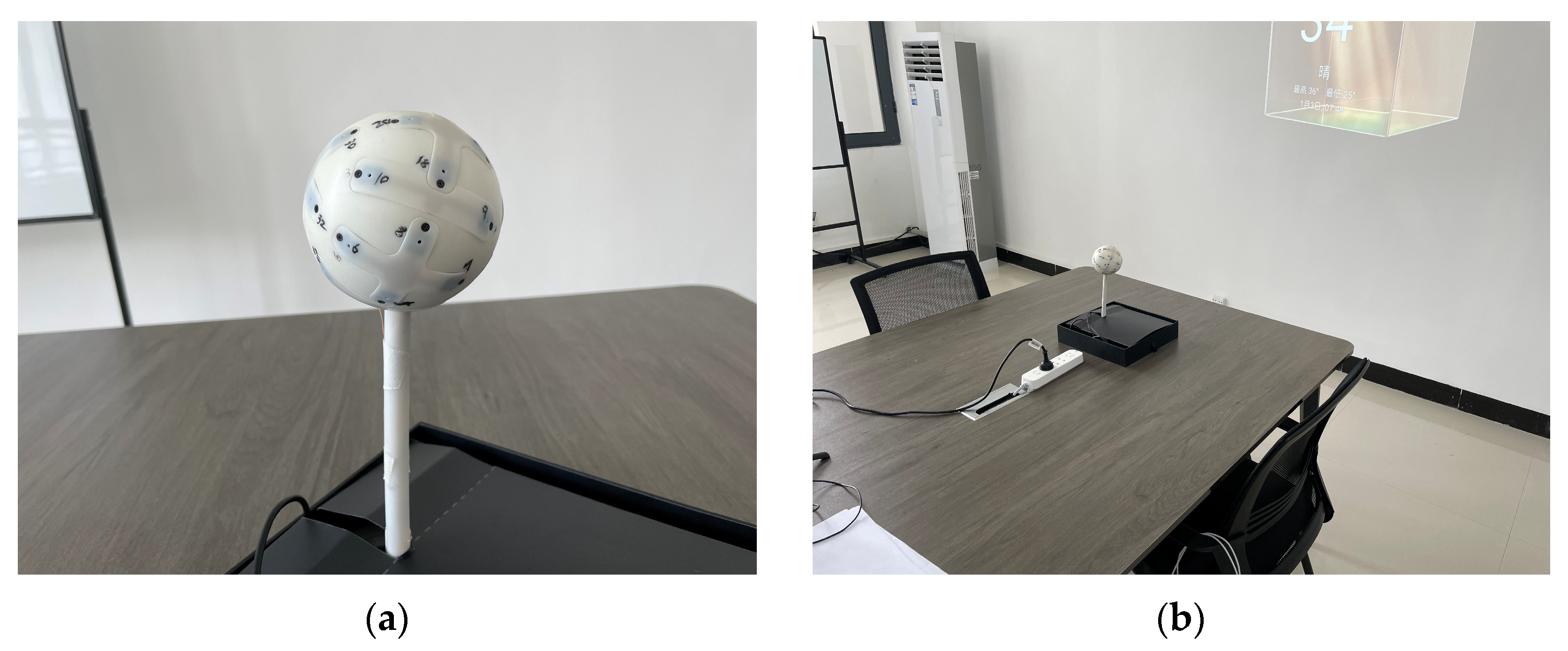
In this section, we used real recordings to verify the effectiveness of the NPTS-ESPRIT algorithm proposed in this paper. The experiment was completed in a conference room of the Guilin University of Electronic Technology. In this experiment, we used a rigid spherical array with a sampling rate of 48,000 Hz and 32 microphones uniformly distributed on the surface to record 4 s long recordings each time. Then we carried out STFT analysis on the collected time-domain records. The parameters of the STFT are as follows: Hanning window length of 1024 samples, 50% overlap between adjacent frames, and FFT of 1024 points. The localization algorithm uses 21 frequency points ranging from 2250 Hz to 3187.5 Hz. The spherical microphone array and experimental site we used are shown in Figure 9.

Firstly, we conducted the test in the single-source scenario. In this scenario, there is a speaker located at (175°, 75°) relative to the center of the spherical array.

Table 3. Single speaker scenario.

Ground Truth DOA	NPTS-ESPRIT/Angular Error	TS-ESPRIT/Angular Error
(175°, 75°)	(174.9062°, 74.9743°)/0.0942°	(174.9062°, 77.5281°)/2.5297°

shows the estimation results of the NPTS-ESPRIT algorithm and TS-ESPRIT algorithm in this scenario and the angular error between the estimated value and the true value, respectively.

Then, we conducted the test in the dual-source scenario. In this scenario, there are two simultaneous speakers located at (235°, 85°) and (125°, 75°) relative to the array center. Table 3 shows the estimation results of the NPTS-ESPRIT algorithm and TS-ESPRIT algorithm in this scenario and the angle error between the estimated value and the true value, respectively. From Table 3 and

Table 4. Dual-source scenario.

Ground Truth DOA	NPTS-ESPRIT/Angular Error	TS-ESPRIT/Angular Error
(175°, 75°)	(174.9062°, 74.9743°)/0.0942°	(174.9062°, 77.5281°)/2.5297°
(125°, 75°)	(126.8516°, 74.8148°)/1.7973°	(126.5452°, 77.1942°)/2.6578°

, we can see that both algorithms successfully detect the location of the sound source in different scenarios and that the estimation error of the NPTS-ESPRIT algorithm is smaller than that of the TS-ESPRIT algorithm.

5. Discussion

In this paper, we write the two eigenvalue decompositions in the TS-ESPRIT algorithm to determine the DOA parameter as a generalized eigenvalue problem, which avoids the two eigenvalue decomposition operations. By using the QZ algorithm to solve the generalized eigenvalue problem, the problem of DOA parameter pairing in TS-ESPRIT is solved without increasing the computational complexity of the algorithm. At the same time, due to the use of the tangent function as the directional parameter, the proposed method has higher and more stable estimation accuracy for the elevation angle compared with traditional algorithms. We also further improve the positioning accuracy of the algorithm in noisy and multi-source scenes by introducing the concept of relative sound pressure. Finally, by introducing frequency-smoothing technology to remove the correlation between signals, our algorithm can be applied to indoor sound source positioning scenes with reverberation. Through rich numerical simulations and field measurements, we demonstrate that the proposed method solves the problem of DOA parameter pairing in TS-ESPRIT techniques and has outstanding DOA estimation accuracy compared with traditional algorithms. In the future, we will further optimize the proposed algorithm to make it better able to complete the positioning and tracking of multiple sound sources in low-SNR and high-reverberation environments.

References

- Evers, C.; Lollmann, H.W.; Mellmann, H.; Schmidt, A.; Barfuss, H.; Naylor, P.A.; Kellermann, W. The LOCATA Challenge: Acoustic Source Localization and Tracking. IEEE/ACM Trans. Audio Speech Lang. Process. 2020, 28, 1620–1643. [Google Scholar] [CrossRef]
- Wang, Z.-Q.; Wang, D. Localization based Sequential Grouping for Continuous Speech Separation. In Proceedings of the 2022 IEEE International Conference on Acoustics, Speech and Signal Processing (ICASSP), Singapore, 22–27 May 2022; pp. 281–285. [Google Scholar] [CrossRef]
- Gannot, S.; Vincent, E.; Markovich-Golan, S.; Ozerov, A. A Consolidated Perspective on Multimicrophone Speech Enhancement and Source Separation. IEEE/ACM Trans. Audio Speech Lang. Process. 2017, 25, 692–730. [Google Scholar] [CrossRef]
- Choi, J.-W.; Zotter, F.; Jo, B.; Yoo, J.-H. Multiarray Eigenbeam-ESPRIT for 3D Sound Source Localization with Multiple Spherical Microphone Arrays. IEEE/ACM Trans. Audio Speech Lang. Process. 2022, 30, 2310–2325. [Google Scholar] [CrossRef]
- Rafaely, B. Analysis and Design of Spherical Microphone Arrays. IEEE Trans. Speech Audio Process. 2005, 13, 135–143. [Google Scholar] [CrossRef]
- Williams, E.G.; Mann, J.A. Fourier Acoustics: Sound Radiation and Nearfield Acoustical Holography. J. Acoust. Soc. Am. 2000, 108, 1373. [Google Scholar] [CrossRef]
- Jaafer, Z.; Goli, S.; Elameer, A.S. Performance Analysis of Beam Scan, MIN-NORM, Music and Mvdr DOA Estimation Algorithms. In Proceedings of the 2018 International Conference on Engineering Technology and Their Applications (IICETA), Al-Najaf, Iraq, 8–9 May 2018; pp. 72–76. [Google Scholar] [CrossRef]
- Khaykin, D.; Rafaely, B. Acoustic Analysis by Spherical Microphone Array Processing of Room Impulse Responses. J. Acoust. Soc. Am. 2012, 132, 261–270. [Google Scholar] [CrossRef]
- He, H.; Wu, L.; Lu, J.; Qiu, X.; Chen, J. Time Difference of Arrival Estimation Exploiting Multichannel Spatio-Temporal Prediction. IEEE Trans. Audio Speech Lang. Process. 2013, 21, 463–475. [Google Scholar] [CrossRef]
- Jarrett, D.P.; Habets, E.A.P.; Thomas, M.R.P.; Naylor, P.A. Rigid Sphere Room Impulse Response Simulation: Algorithm and Applications. J. Acoust. Soc. Am. 2012, 132, 1462–1472. [Google Scholar] [CrossRef]
- Tervo, S.; Politis, A. Direction of Arrival Estimation of Reflections from Room Impulse Responses Using a Spherical Microphone Array. IEEE/ACM Trans. Audio Speech Lang. Process. 2015, 23, 1539–1551. [Google Scholar] [CrossRef]
- Sun, H.; Teutsch, H.; Mabande, E.; Kellermann, W. Robust Localization of Multiple Sources in Reverberant Environments Using EB-ESPRIT with Spherical Microphone Arrays. In Proceedings of the 2011 IEEE International Conference on Acoustics, Speech and Signal Processing (ICASSP), Prague, Czech Republic, 22–27 May 2011; pp. 117–120. [Google Scholar] [CrossRef]
- Huang, Q.; Zhang, L.; Fang, Y. Two-Stage Decoupled DOA Estimation Based on Real Spherical Harmonics for Spherical Arrays. IEEE/ACM Trans. Audio Speech Lang. Process. 2017, 25, 2045–2058. [Google Scholar] [CrossRef]
- Huang, Q.; Zhang, L.; Fang, Y. Two-Step Spherical Harmonics ESPRIT-Type Algorithms and Performance Analysis. IEEE/ACM Trans. Audio Speech Lang. Process. 2018, 26, 1684–1697. [Google Scholar] [CrossRef]
- Teutsch, H.; Kellermann, W. Eigen-beam processing for direction-of-arrival estimation using spherical apertures. In Proceedings of the 1st Joint Workshop Hands-Free Speech Communication Microphone Arrays (HSCMA), Piscataway, NJ, USA, 17–18 March 2005; pp. 1–2. [Google Scholar]
- Khaykin, D.; Rafaely, B. Coherent Signals Direction-of-Arrival Estimation Using a Spherical Microphone Array: Frequency Smoothing Approach. In Proceedings of the 2009 IEEE Workshop on Applications of Signal Processing to Audio and Acoustics, New Paltz, NY, USA, 18–21 October 2009; pp. 221–224. [Google Scholar] [CrossRef]
- Hu, Y.; Abhayapala, T.D.; Samarasinghe, P.N. Multiple Source Direction of Arrival Estimations Using Relative Sound Pressure Based MUSIC. IEEE/ACM Trans. Audio Speech Lang. Process. 2021, 29, 253–264. [Google Scholar] [CrossRef]
- Duraiswami, R.; Li, Z.; Zotkin, D.N.; Grassi, E.; Gumerov, N.A. Plane-Wave Decomposition Analysis for Spherical Microphone Arrays. In Proceedings of the IEEE Workshop on Applications of Signal Processing to Audio and Acoustics, 2005, New Paltz, NY, USA, 16–19 October 2005; pp. 150–153. [Google Scholar]
- Tervo, S. Direction Estimation Based on Sound Intensity Vectors. In Proceedings of the 2009 European Signal Processing Conference (EUSIPCO-2009), Glasgow, UK, 24–28 August 2009. [Google Scholar]
- Wabnitz, A.; Epain, N.; McEwan, A.; Jin, C. Upscaling Ambisonic Sound Scenes Using Compressed Sensing Techniques. In Proceedings of the 2011 IEEE Workshop on Applications of Signal Processing to Audio and Acoustics (WASPAA), New Paltz, NY, USA, 16–19 October 2011; pp. 1–4. [Google Scholar] [CrossRef]
- Famoriji, O.J.; Shongwe, T. Subspace Pseudointensity Vectors Approach for DoA Estimation Using Spherical Antenna Array in the Presence of Unknown Mutual Coupling. Appl. Sci. 2022, 12, 10099. [Google Scholar] [CrossRef]
- Famoriji, O.J.; Shongwe, T. Critical Review of Basic Methods on DoA Estimation of EM Waves Impinging a Spherical Antenna Array. Electronics 2022, 11, 208. [Google Scholar] [CrossRef]
- Jo, B.; Choi, J.-W. Parametric Direction-of-Arrival Estimation with Three Recurrence Relations of Spherical Harmonics. J. Acoust. Soc. Am. 2019, 145, 480–488. [Google Scholar] [CrossRef] [PubMed]
- Jo, B.; Choi, J.-W. Direction of Arrival Estimation Using Nonsingular Spherical ESPRIT. J. Acoust. Soc. Am. 2018, 143, EL181–EL187. [Google Scholar] [CrossRef]
- Rafaely, B. Plane-Wave Decomposition of the Sound Field on a Sphere by Spherical Convolution. J. Acoust. Soc. Am. 2004, 116, 2149–2157. [Google Scholar] [CrossRef]
- Samarasinghe, P.; Abhayapala, T.; Poletti, M. Wavefield Analysis Over Large Areas Using Distributed Higher Order Microphones. IEEE/ACM Trans. Audio Speech Lang. Process. 2014, 22, 647–658. [Google Scholar] [CrossRef]
- Madmoni, L.; Rafaely, B. Direction of Arrival Estimation for Reverberant Speech Based on Enhanced Decomposition of the Direct Sound. IEEE J. Sel. Top. Signal Process. 2019, 13, 131–142. [Google Scholar] [CrossRef]
- Rafaely, B.; Alhaiany, K. Speaker Localization Using Direct Path Dominance Test Based on Sound Field Directivity. Signal Process. 2018, 143, 42–47. [Google Scholar] [CrossRef]
- Rafaely, B. Spatial Sampling and Beamforming for Spherical Microphone Arrays. In Proceedings of the 2008 Hands-Free Speech Communication and Microphone Arrays, Trento, Italy, 6–8 May 2008; pp. 5–8. [Google Scholar] [CrossRef]
- Choi, C.H.; Ivanic, J.; Gordon, M.S.; Ruedenberg, K. Rapid and Stable Determination of Rotation Matrices between Spherical Harmonics by Direct Recursion. J. Chem. Phys. 1999, 111, 8825–8831. [Google Scholar] [CrossRef]
- Li, R.C. Matrix Perturbation Theory: Generalized Eigenvalue Problems. In Handbook of Linear Algebra; Hogben, L., Ed.; Chapman and Hall/CRC: Boca Raton, FL, USA, 2007; Chapter 15. [Google Scholar]
- Moler, C.B.; Stewart, G.W. An Algorithm for Generalized Matrix Eigenvalue Problems. SIAM J. Numer. Anal. 1973, 10, 241–256. [Google Scholar] [CrossRef]
- Diaz-Guerra, D.; Miguel, A.; Beltran, J.R. Robust Sound Source Tracking Using SRP-PHAT and 3D Convolutional Neural Networks. IEEE/ACM Trans. Audio Speech Lang. Process. 2021, 29, 300–311. [Google Scholar] [CrossRef]
- Hardin, R.H.; Sloane, N.J.A. McLaren’s Improved Snub Cube and Other New Spherical Designs in Three Dimensions. Discret. Comput. Geom. 1996, 15, 429–441. [Google Scholar] [CrossRef]
- Herzog, A.; Habets, E. Online DOA Estimation Using Real Eigenbeam ESPRIT with Propagation Vector Matching. In Proceedings of the EAA Spatial Audio Signal Processing Symposium, Paris, France, 6–7 September 2019; pp. 19–24. [Google Scholar] [CrossRef]
- Johnson, B.A.; Abramovich, Y.I.; Mestre, X. MUSIC, G-MUSIC, and Maximum-Likelihood Performance Breakdown. IEEE Trans. Signal Process. 2008, 56, 3944–3958. [Google Scholar] [CrossRef]
- Markovich, S.; Gannot, S.; Cohen, I. Multichannel Eigenspace Beamforming in a Reverberant Noisy Environment with Multiple Interfering Speech Signals. IEEE Trans. Audio Speech Lang. Process. 2009, 17, 1071–1086. [Google Scholar] [CrossRef]
Figure 1.
MAEEs for various source elevation angles and their SNRs. (a) Elevation errors at SNR = 0 dB; (b) Elevation errors at SNR = 20 dB; (c) Azimuth errors at SNR = 0 dB; (d) Azimuth errors at SNR = 20 dB.
Figure 2.
MAEEs of two incoherent sound sources at different SNRs. (a) Azimuth errors at different SNRs; (b) Elevation errors at different SNRs.
Figure 3.
MAEEs of two incoherent sound sources at different snapshots. (a) Azimuth errors at different snapshots; (b) Elevation errors at different snapshots.
Figure 4.
Hash map of NPTS−ESPRIT (each red circle denotes a theoretical DOA, and each blue × denotes an estimated DOA of NPTS−ESPRIT).
Figure 5.
Mean angular error under two different reverberation times.
Figure 6.
Normalized eigenvalues obtained via a singular value decomposition of the source signal covariance matrix (room reverberations T60 = 0.3 s): (a) SNR = 0 dB; (b) SNR = 5 dB; (c) SNR = 10 dB; (d) SNR =15 dB; (e) SNR = 20 dB.
Figure 7.
The overall MAEE about angles under different SNRs with two sources at (70°, 130°) and (170°, 55°).
Figure 8.
MAEE for the angles of interest at (90°, 165°), (−70°, 135°), (130°, 110°), (−30°, 80°), and (170°, 55°) for the presence of five sources with different SNRs.
Figure 9.
Field testing. (a) Spherical microphone array; (b) Conference room.