The Implicit Numerical Method for the Radial Anomalous Subdiffusion Equation

Abstract

This paper presents a numerical method for solving a two-dimensional subdiffusion equation with a Caputo fractional derivative. The problem considered assumes symmetry in both the equation’s solution domain and the boundary conditions, allowing for a reduction of the two-dimensional equation to a one-dimensional one. The proposed method is an extension of the fractional Crank–Nicolson method, based on the discretization of the equivalent integral-differential equation. To validate the method, the obtained results were compared with a solution obtained through the Laplace transform. The analytical solution in the image of the Laplace transform was inverted using the Gaver–Wynn–Rho algorithm implemented in the specialized mathematical computing environment, Wolfram Mathematica. The results clearly show the mutual convergence of the solutions obtained via the two methods.

1. Introduction

Diffusion is a process of spontaneous movement of particles due to collisions with other particles. These collisions can occur between diffusing particles as well as particles of the medium in which diffusion occurs. The fundamental characteristic of this type of movement is that the mean square displacement of the particle (the square of its dispersion) depends non-linearly on time [1,2]

$$〈x^2\left(t\right)〉\sim D_{\alpha }{t}^{\alpha },0<\alpha \le 2,$$

(1)

as opposed to the linear dependence ($\alpha =1$) that characterizes Brownian motion. In the first case, when the exponent of the power is less than one, it is called subdiffusion, whereas when the diffusion exponent is greater than one, it is called superdiffusion. The second case concerns the so-called Lévy flights, which have been observed experimentally [3,4,5]. Subdiffusion is most commonly observed in media such as gels and porous media, where particle movement is extremely difficult [6,7].

Thermal conductivity, which involves the flow of heat through solid substances like metal, is a twin process to diffusion. It is a process where thermal energy is transferred through conduction by the transfer of particle vibrations. The particles in a solid state are close to each other and are held together by intermolecular forces. When one particle gains energy, it transfers it to the neighboring particle through vibration transfer. Mathematical models incorporating fractional-order derivatives are excellent tools for describing thermal conduction in porous materials, such as porous aluminum [8].

Within the framework of subdiffusion or thermal conductivity processes modeled by subdiffusion or the fractional thermal conductivity equation, a subclass of so-called fractional Stefan problems can be distinguished. They are designed to describe the evolution of the boundary between two phases of a material undergoing a phase transition. Examples include the drug release from slab matrices [9,10]. Numerous papers presenting analytical and numerical results have been devoted to this phenomenon [11,12,13,14,15,16,17].

In the papers [18,19], Povstenko et al. consider the two dimensional time-fractional heat conduction equations. In the solution, they use Laplace and Fourier integral transforms, which facilitate the reduction of higher-degree differential equations to lower-degree equations, thus greatly improved the obtaining of the solution. The paper [19] uses the Gaver–Stehfest algorithm to invert the Laplace transform. A similar approach to those presented in the aforementioned papers is used in this article, based, moreover, on the results presented in the monograph [20], with the difference being that the Gaver–Wynn–Rho algorithm [21,22,23] was used to determine the original solution from the Laplace transform image. The other analytical method used in the context of fractional partial differential equations is the method of the separation of variables [24,25].

Numerous numerical methods have been proposed for solving equations of anomalous diffusion. Ciesielski introduced numerical schemes for various cases in his doctoral dissertation [26], including equations with fractional-order time and spatial derivatives. The discussed cases were limited to one-dimensional problems. Papers [27,28] considered one-dimensional subdiffusion equations with a fractional spatial Riemann–Liouville derivative and provided corresponding numerical schemes. Bhrawy et al. [29] presented a numerical method for a subdiffusion equation with a Caputo time derivative. Błasik [30,31,32] extended the classical Crank–Nicolson method to one-dimensional subdiffusion equations with a Caputo time derivative, considering a variable diffusion coefficient and nonlinear source term. Other variants of the Crank–Nicolson method for the subdiffusion equation are included in the papers [33,34,35]. Noteworthy are also the articles [36,37,38,39,40], in which the authors have developed numerical methods characterized by high accuracy. Numerical results for the two-dimensional subdiffusion equation were presented in papers [41,42], while a more general case involving a source term was discussed in [43,44].

Other methods for solving the anomalous diffusion equation include meshless techniques [45,46,47], such as the Singular Boundary Method (SBM), Radial Basis Function (RBF) and the Moving Particle Semi-Implicit (MPS) approach do not require conventional structured meshes for problem domain discretization. Other examples of using meshless methods with Chebyshev and Lagrange polynomials are developed in papers [48,49].

The article is structured as follows. The Section 2 presents the basic definitions and properties of the following: fractional order differential calculus, integral transforms, and numerical methods. These concepts are utilized throughout the rest of the article. In the subsequent section, the problem to be solved is formulated as a two-dimensional sub-diffusion equation, along with uniqueness conditions. Two different solutions were employed to solve this problem, and each one is discussed in its respective sub-section. The Section 4 and Section 5 showcase the numerical results obtained from the calculations and convergence analysis of the proposed numerical scheme. Finally, the article concludes with a section summarizing the findings and providing additional insights.

2. Preliminaries

Let us begin our consideration by introducing two fractional order operators: the left-sided Riemann–Liouville integral and the left-sided Caputo derivative together with the composition rule of the two mentioned operators [50].

Definition 1.

The left-sided Riemann–Liouville integral of order α, denoted as $I_{0+}^{\alpha }$, is given by the following formula for $Re\left(\alpha \right)\in (0,1]$:

$$I_{0+}^{\alpha }f\left(t\right):=\frac{1}{\Gamma \left(\alpha \right)}{\int }_0^t\frac{f\left(\tau \right)d\tau }{{(t-\tau )}^{1-\alpha }},$$

(2)

where $\Gamma$ is the Euler gamma function.

Definition 2.

Let $Re\left(\alpha \right)\in (0,1]$. The left-sided Caputo derivative of order α is given by the formula:

$${}^C{D}_{0+}^{\alpha }f\left(t\right):=\left\{\begin{array}{cc}\frac{1}{\Gamma (1-\alpha )}{\int }_0^t\frac{f^{{}^{\prime }}\left(\tau \right)d\tau }{{(t-\tau )}^{\alpha }},\hfill & 0<Re\left(\alpha \right)<1,\hfill \\ \frac{df\left(t\right)}{dt},\hfill & Re\left(\alpha \right)=1.\hfill \end{array}\right.$$

(3)

Property 1

([50] Lemma 2.22). Let function $f\in C^1(0,T)$. Then, the composition rule for the left-sided Riemann–Liouville integral and the left-sided Caputo derivative is given as follows:

$$I_{0+}^{\alpha }{}^C{D}_{0+}^{\alpha }f\left(t\right)=f\left(t\right)-f\left(0\right),Re\left(\alpha \right)\in (0,1].$$

(4)

The definition of the Laplace integral transform [51], combined with the following property [52], will play an important role in determining the semi-analytical solution of the problem considered in the next section.

Definition 3.

Let $f\left(t\right)$ be a real function of the variable $t\in \mathbb{R}$. Then, the Laplace transform of the function $f\left(t\right)$ is the function $\widehat{f}\left(s\right)$ of the complex variable defined by formula

$$\mathcal{L}\left\{f\left(t\right)\right\}=\widehat{f}\left(s\right)={\int }_0^{\infty }{e}^{-st}f\left(t\right)dt,$$

(5)

where $Re\left(s\right)>0$.

Property 2.

Let the function $f\left(t\right)$ be the original, and let $\mathcal{L}\left\{f\left(t\right)\right\}=\widehat{f}\left(s\right)$, then the following formula holds

$$\mathcal{L}\left\{{}^C{D}_{0+}^{\alpha }f\left(t\right)\right\}=s^{\alpha }\widehat{f}\left(s\right)-s^{\alpha -1}f\left(0\right),Re\left(\alpha \right)\in (0,1].$$

(6)

Bessel functions of the first and second kind [50,53] present two further definitions.

Definition 4.

Let $z\in \mathbb{C}\setminus \{{\mathbb{R}}_{-},0\}$ and $\nu \in \mathbb{C}$, then the Bessel function of the first kind denoted by $J_{\nu }\left(z\right)$ is given by the following series:

$$J_{\nu }\left(z\right)=\sum _{l=0}^{\infty }\frac{{(-1)}^l{(z/2)}^{2l+\nu }}{l!\Gamma (\nu +l+1)}.$$

(7)

Definition 5.

Let $\nu \in \mathbb{C}\setminus \mathbb{Z}$, then the Bessel function of the second kind denoted by $Y_{\nu }\left(z\right)$ is given by the following formula:

$$Y_{\nu }\left(z\right)=\frac{J_{\nu }\left(z\right)cos\nu \pi -J_{-\nu }\left(z\right)}{sin\nu \pi }.$$

(8)

In the case of integer order $m\in \mathbb{Z}$, function is defined in terms of the limit of

$$Y_m\left(z\right)=\underset{\nu \to m}{lim}{Y}_{\nu }\left(z\right).$$

(9)

The numerical scheme proposed in the next section uses a mesh of nodes defined as follows:

Definition 6.

Let $\Pi =\{(r,t):r\in \left[\frac{1}{2},1\right];t\in [0,1]\}$ be a continuous region of solutions for the partial differential equation. Then, the set $\overline{\Pi }=\{(r_i,t_j)\in \Pi :r_i=\frac{1}{2}+i\Delta r,i\in \{0,1,\cdots ,m\},$ $\Delta r=\frac{1}{2m};t_j=j\Delta t,j\in \{0,1,\cdots ,n\};\Delta t=\frac{1}{n}\}$, which we call the rectangular regular mesh described by the set of nodes.

In the following part of the paper, the real order of the left-sided Caputo derivative and the left-sided Riemann–Liouville integral is considered.

3. Mathematical Formulation and Solution of the Problem

Consider a two-dimensional subdiffusion equation in a region with axial symmetry. Let us also assume an axisymmetric system of boundary and initial conditions. The equation under consideration has the form:

$${}^C{D}_{0+,t}^{\alpha }U(x,y,t)=D_{\alpha }\left(\frac{{\partial }^{2}U(x,y,t)}{\partial x^2}+\frac{{\partial }^{2}U(x,y,t)}{\partial y^2}\right),\frac{1}{4}<x^2+y^2<1,t>0,$$

(10)

supplemented by boundary conditions on the edges of the circular ring:

$$U(x,y,t)=U_b,x^2+y^2=1,t>0,$$

(11)

$$U(x,y,t)=0,x^2+y^2=\frac{1}{4},t>0,$$

(12)

and initial condition

$$U(x,y,0)=0,\frac{1}{4}\le x^2+y^2\le 1,$$

(13)

where the generalized diffusion coefficient $D_{\alpha }$ is constant.

In the axisymmetric region in which we derive the solution of the differential equation, it is convenient to introduce the polar coordinates given by $x=rcos\varphi$, $y=rsin\varphi$, for which the differential Equation (10) with boundary and initial conditions takes the form of:

$$\begin{array}{cc}\hfill & {}^C{D}_{0+,t}^{\alpha }U(r,\varphi ,t)=D_{\alpha }\left(\frac{{\partial }^{2}U(r,\varphi ,t)}{\partial r^2}+\frac{1}{r^2}\frac{{\partial }^{2}U(r,\varphi ,t)}{\partial {\varphi }^2}+\frac{1}{r}\frac{\partial U(r,\varphi ,t)}{\partial r}\right),\hfill \\ & \frac{1}{2}<r<1,0\le \varphi <2\pi ,t>0,\hfill \end{array}$$

(14)

$$U(1,\varphi ,t)=U_b,0\le \varphi <2\pi ,t>0,$$

(15)

$$U\left(\frac{1}{2},\varphi ,t\right)=0,0\le \varphi <2\pi ,t>0,$$

(16)

$$U\left(r,\varphi ,0\right)=0,\frac{1}{2}\le r\le 1,0\le \varphi <2\pi .$$

(17)

The assumptions made about symmetry allow us to reduce the dimension of the problem under consideration. Let us note that for a fixed radius r and arbitrary angle $\varphi$, the diffusion flux in the direction normal to the edge takes the constant values. Thus, the function U does not depend on $\varphi$, and the second differential term on the right hand side of Equation (14) is equal to zero. As a result, the two-dimensional equation is immediately reduced to the one-dimensional one:

$$\begin{array}{cc}\hfill & {}^C{D}_{0+,t}^{\alpha }U(r,t)=D_{\alpha }\left(\frac{{\partial }^{2}U(r,t)}{\partial r^2}+\frac{1}{r}\frac{\partial U(r,t)}{\partial r}\right),\frac{1}{2}<r<1,t>0,\hfill \end{array}$$

(18)

$$U(1,t)=U_b,t>0,$$

(19)

$$U\left(\frac{1}{2},t\right)=0,t>0,$$

(20)

$$U\left(r,0\right)=0,\frac{1}{2}\le r\le 1.$$

(21)

It should be mentioned that in addition to symmetry, there are other ways to reduce the dimensions of differential problems, such as scaling [54,55] and integral transforms [51], which will be shown in the next section.

3.1. A Numerical Approach

In the paper [30], a generalized Crank–Nicolson method was proposed for the one-dimensional subdiffusion equation. The obtained results were further extended to the more general case, to the equation with a source term [31]. In both cases, obtained results confirmed the accuracy of the proposed methods. Therefore, an analogous approach will be applied to the problem defined by Equations (18)–(21).

For some technical reasons, the numerical approximation of the left-sided Caputo derivative is much simpler compared to the approximation of the left-sided Riemann–Liouville integral. Therefore, we apply Property 1 to the Equation (18), which yields an integro-differential equation in the following form:

$$\begin{array}{cc}\hfill U(r,t)& =U(r,0)+\frac{D_{\alpha }}{\Gamma \left(\alpha \right)}{\int }_0^t\frac{1}{{(t-\tau )}^{1-\alpha }}\frac{{\partial }^{2}U(r,\tau )}{\partial r^2}d\tau \hfill \\ & +\frac{D_{\alpha }}{r\Gamma \left(\alpha \right)}{\int }_0^t\frac{1}{{(t-\tau )}^{1-\alpha }}\frac{\partial U(r,\tau )}{\partial r}d\tau .\hfill \end{array}$$

(22)

The solution U of the initial boundary value problem considered in the paper fulfills the assumptions of Property 1, and its existence and the uniqueness was proven in the more general case in the paper [56]. Further consideration will be conducted with reference to the mesh of nodes given in Definition 6. For each node of the grid, we determine the discrete form of the integral kernel in the integrals on the right-hand side of Equation (22). For this purpose, we approximate the solution U using a linear function between two consecutive nodes with respect to the variable t:

$$\overline{U}(r,t)=U(r,t_j)\frac{t-t_{j+1}}{t_j-t_{j+1}}+U(r,t_{j+1})\frac{t-t_j}{t_{j+1}-t_j},$$

(23)

for $t_j\le t\le t_{j+1}$, $j=0,\cdots ,n-1$. The first integral term of Equation (22) on the interval $[0,t_k]$ can be approximated by the formula:

$$\begin{array}{cc}\hfill & \frac{D_{\alpha }}{\Gamma \left(\alpha \right)}{\int }_0^{t_k}\frac{1}{{(t_k-\tau )}^{1-\alpha }}\frac{{\partial }^{2}U(r,\tau )}{\partial r^2}d\tau \approx \frac{D_{\alpha }}{\Gamma \left(\alpha \right)}{\int }_0^{t_k}\frac{1}{{(t_k-\tau )}^{1-\alpha }}\frac{{\partial }^2\overline{U}(r,\tau )}{\partial r^2}d\tau .\hfill \end{array}$$

(24)

From the theorem on additivity of an integral with respect to the integration interval, we obtain:

$$\begin{array}{cc}& \frac{D_{\alpha }}{\Gamma \left(\alpha \right)}{\int }_0^{t_k}\frac{1}{{(t_k-\tau )}^{1-\alpha }}\frac{{\partial }^2\overline{U}(r,\tau )}{\partial r^2}d\tau =\frac{D_{\alpha }}{\Gamma \left(\alpha \right)}\sum _{j=0}^{k-1}{\int }_{t_j}^{t_{j+1}}\frac{1}{{(t_k-\tau )}^{1-\alpha }}\left(\frac{{\partial }^{2}U(r,t_j)}{\partial r^2}\frac{\tau -t_{j+1}}{t_j-t_{j+1}}\right.+\hfill \\ & \left.\frac{{\partial }^{2}U(r,t_{j+1})}{\partial r^2}\frac{\tau -t_j}{t_{j+1}-t_j}\right)d\tau =\frac{D_{\alpha }}{\Gamma \left(\alpha \right)}\frac{{\partial }^{2}U(r,t_0)}{\partial r^2}{\int }_0^{t_1}\frac{1}{{(t_k-\tau )}^{1-\alpha }}\frac{\tau -t_1}{t_0-t_1}d\tau +\hfill \\ & \frac{D_{\alpha }}{\Gamma \left(\alpha \right)}\sum _{j=1}^{k-1}\frac{{\partial }^{2}U(r,t_j)}{\partial r^2}\left({\int }_{t_{j-1}}^{t_j}\frac{1}{{(t_k-\tau )}^{1-\alpha }}\frac{\tau -t_{j-1}}{t_j-t_{j-1}}d\tau \right.+\left.{\int }_{t_j}^{t_{j+1}}\frac{1}{{(t_k-\tau )}^{1-\alpha }}\frac{\tau -t_{j+1}}{t_j-t_{j+1}}d\tau \right)+\hfill \\ & \frac{D_{\alpha }}{\Gamma \left(\alpha \right)}\frac{{\partial }^{2}U(r,t_k)}{\partial r^2}{\int }_{t_{k-1}}^{t_k}\frac{1}{{(t_k-\tau )}^{1-\alpha }}\frac{\tau -t_{k-1}}{t_k-t_{k-1}}d\tau .\hfill \end{array}$$

The second integral term of Equation (22) on the interval $[0,t_k]$ can be approximated by the formula:

$$\begin{array}{cc}\hfill & \frac{D_{\alpha }}{r\Gamma \left(\alpha \right)}{\int }_0^{t_k}\frac{1}{{(t_k-\tau )}^{1-\alpha }}\frac{\partial U(r,\tau )}{\partial r}d\tau \approx \frac{D_{\alpha }}{r\Gamma \left(\alpha \right)}{\int }_0^{t_k}\frac{1}{{(t_k-\tau )}^{1-\alpha }}\frac{\partial \overline{U}(r,\tau )}{\partial r}d\tau .\hfill \end{array}$$

(25)

Applying again the theorem on additivity of an integral with respect to the integration interval, we obtain:

$$\begin{array}{cc}& \frac{D_{\alpha }}{r\Gamma \left(\alpha \right)}{\int }_0^{t_k}\frac{1}{{(t_k-\tau )}^{1-\alpha }}\frac{\partial \overline{U}(r,\tau )}{\partial r}d\tau =\frac{D_{\alpha }}{r\Gamma \left(\alpha \right)}\sum _{j=0}^{k-1}{\int }_{t_j}^{t_{j+1}}\frac{1}{{(t_k-\tau )}^{1-\alpha }}\left(\frac{\partial U(r,t_j)}{\partial r}\frac{\tau -t_{j+1}}{t_j-t_{j+1}}\right.+\hfill \\ & \left.\frac{\partial U(r,t_{j+1})}{\partial r}\frac{\tau -t_j}{t_{j+1}-t_j}\right)d\tau =\frac{D_{\alpha }}{r\Gamma \left(\alpha \right)}\frac{\partial U(r,t_0)}{\partial r}{\int }_0^{t_1}\frac{1}{{(t_k-\tau )}^{1-\alpha }}\frac{\tau -t_1}{t_0-t_1}d\tau +\hfill \end{array}$$

$$\begin{array}{cc}& \frac{D_{\alpha }}{r\Gamma \left(\alpha \right)}\sum _{j=1}^{k-1}\frac{\partial U(r,t_j)}{\partial r}\left({\int }_{t_{j-1}}^{t_j}\frac{1}{{(t_k-\tau )}^{1-\alpha }}\frac{\tau -t_{j-1}}{t_j-t_{j-1}}d\tau \right.+\left.{\int }_{t_j}^{t_{j+1}}\frac{1}{{(t_k-\tau )}^{1-\alpha }}\frac{\tau -t_{j+1}}{t_j-t_{j+1}}d\tau \right)+\hfill \\ & \frac{D_{\alpha }}{r\Gamma \left(\alpha \right)}\frac{\partial U(r,t_k)}{\partial r}{\int }_{t_{k-1}}^{t_k}\frac{1}{{(t_k-\tau )}^{1-\alpha }}\frac{\tau -t_{k-1}}{t_k-t_{k-1}}d\tau .\hfill \end{array}$$

Calculating the following integrals:

$$\begin{array}{cc}\hfill & w_{0,k}=\frac{1}{\Gamma \left(\alpha \right)}{\int }_0^{t_1}\frac{1}{{(t_k-\tau )}^{1-\alpha }}\frac{\tau -t_1}{t_0-t_1}d\tau =\frac{{(\Delta t)}^{\alpha }}{\Gamma (2+\alpha )}\left((\alpha +1-k)k^{\alpha }+{(k-1)}^{\alpha +1}\right),\hfill \end{array}$$

(26)

$$\begin{array}{cc}\hfill & w_{j,k}=\frac{1}{\Gamma \left(\alpha \right)}\left({\int }_{t_{j-1}}^{t_j}\frac{1}{{(t_k-\tau )}^{1-\alpha }}\frac{\tau -t_{j-1}}{t_j-t_{j-1}}d\tau +\right.\left.{\int }_{t_j}^{t_{j+1}}\frac{1}{{(t_k-\tau )}^{1-\alpha }}\frac{\tau -t_{j+1}}{t_j-t_{j+1}}d\tau \right)=\hfill \\ & \frac{{(\Delta t)}^{\alpha }}{\Gamma (2+\alpha )}\left({(k-j+1)}^{\alpha +1}-\right.\left.2{(k-j)}^{\alpha +1}+{(k-j-1)}^{\alpha +1}\right),\mathrm{for}0<j<k,\hfill \end{array}$$

(27)

$$\begin{array}{cc}\hfill & w_{k,k}=\frac{1}{\Gamma \left(\alpha \right)}{\int }_{t_{k-1}}^{t_k}\frac{1}{{(t_k-\tau )}^{1-\alpha }}\frac{\tau -t_{k-1}}{t_k-t_{k-1}}d\tau =\frac{{(\Delta t)}^{\alpha }}{\Gamma (2+\alpha )},\hfill \end{array}$$

(28)

where $t_j=j\Delta t$, and $0\le j\le k$, we receive the values of the integral kernel of the left-sided Riemann–Liouville integral, determined for the suitable grid nodes corresponding to the time variable t.

Subsequently, we discretize the first- and second-order derivatives of the right-hand side of the integro-differential Equation (22) using differential quotients approximating the first

$${\left(\frac{\partial U(r,t)}{\partial r}\right)}_{i,j}=\frac{U_{i+1,j}-U_{i-1,j}}{2\Delta r}+O\left({(\Delta r)}^2\right),$$

(29)

and second derivative

$${\left(\frac{{\partial }^{2}U(r,t)}{\partial r^2}\right)}_{i,j}=\frac{U_{i-1,j}-2U_{i,j}+U_{i+1,j}}{{(\Delta r)}^2}+O\left({(\Delta r)}^2\right),$$

(30)

with respect to the spatial variable r.

Using approximations of the corresponding derivatives and the left-sided Riemann–Liouville integrals, we obtain the discrete form of integro-differential Equation (22) as follows:

$$\begin{array}{cc}\hfill & U_{i,k}=U_{i,0}+D_{\alpha }\sum _{j=0}^k{w}_{j,k}\frac{U_{i-1,j}-2U_{i,j}+U_{i+1,j}}{{(\Delta r)}^2}+\frac{D_{\alpha }}{r_i}\sum _{j=0}^k{w}_{j,k}\frac{U_{i+1,j}-U_{i-1,j}}{2\Delta r},\hfill \end{array}$$

(31)

where the weights corresponding to the integral kernel of the left-sided Riemann–Liouville integrals are of the form:

$$w_{j,k}:=\frac{{(\Delta t)}^{\alpha }}{\Gamma (2+\alpha )}\left\{\begin{array}{cc}(\alpha +1-k)k^{\alpha }+{(k-1)}^{\alpha +1},\hfill & j=0\hfill \\ {(k-j+1)}^{\alpha +1}-2{(k-j)}^{\alpha +1}+\hfill & \\ {(k-j-1)}^{\alpha +1},\hfill & 0<j<k\hfill \\ 1,\hfill & j=k\hfill \end{array}\right.$$

(32)

We transform Equation (31) in such a way that the unknown values of the U function in the k-th time layer are on its left side. Finally, we obtain an implicit numerical scheme, which in node $\left(\frac{1}{2}+i\Delta r,k\Delta t\right)$ takes the form:

$$\begin{array}{cc}\hfill & -\frac{D_{\alpha }(2r_i-\Delta r)w_{k,k}}{2r_i{(\Delta r)}^2}{U}_{i-1,k}+\left(1+\frac{2D_{\alpha }{w}_{k,k}}{{(\Delta r)}^2}\right)U_{i,k}-\frac{D_{\alpha }(2r_i+\Delta r)w_{k,k}}{2r_i{(\Delta r)}^2}{U}_{i+1,k}=\hfill \\ & U_{i,0}+\sum _{j=0}^{k-1}\frac{D_{\alpha }{w}_{j,k}}{{(\Delta r)}^2}\left(\frac{2r_i-\Delta r}{2r_i}{U}_{i-1,j}-2U_{i,j}+\frac{2r_i+\Delta r}{2r_i}{U}_{i+1,j}\right).\hfill \end{array}$$

(33)

Applying the above relationship to each of the $m-2$ nodes of the k-th time layer, we obtain a system of linear equations with $m-2$ unknown values of the U-function, which can be written in matrix form:

$$\mathbf{A}{\mathbf{U}}_k=\mathbf{B},$$

(34)

where matrix A is defined by

$$\mathbf{A}=\left[\begin{array}{cccccccc}1+2\delta & -\frac{(2r_1+\Delta r)\delta }{2r_1}& 0& 0& \cdots & 0& 0& 0\\ -\frac{(2r_2-\Delta r)\delta }{2r_2}& 1+2\delta & -\frac{(2r_2+\Delta r)\delta }{2r_2}& 0& \cdots & 0& 0& 0\\ 0& -\frac{(2r_3-\Delta r)\delta }{2r_3}& 1+2\delta & -\frac{(2r_3+\Delta r)\delta }{2r_3}& \cdots & 0& 0& 0\\ ⋮& ⋮& ⋮& ⋮& \ddots & ⋮& ⋮& ⋮\\ 0& 0& 0& -\frac{(2r_i-\Delta r)\delta }{2r_i}& 1+2\delta & -\frac{(2r_i+\Delta r)\delta }{2r_i}& 0& 0\\ ⋮& ⋮& ⋮& ⋮& \ddots & ⋮& ⋮& ⋮\\ 0& 0& 0& 0& \cdots & -\frac{(2r_{m-2}-\Delta r)\delta }{2r_{m-2}}& 1+2\delta & -\frac{(2r_{m-2}+\Delta r)\delta }{2r_{m-2}}\\ 0& 0& 0& 0& \cdots & 0& -\frac{(2r_{m-1}-\Delta r)\delta }{2r_{m-1}}& 1+2\delta \end{array}\right],$$

where $\delta :=\frac{D_{\alpha }{w}_{k,k}}{{(\Delta r)}^2}$. The elements of vector B are defined by

$$\mathbf{B}=\left[\begin{array}{c}{b}_1+\frac{(2r_1-\Delta r)\delta }{2r_1}{U}_{0,k}\\ b_2\\ b_3\\ ⋮\\ b_i\\ ⋮\\ b_{m-2}\\ b_{m-1}+\frac{(2r_{m-1}+\Delta r)\delta }{2r_{m-1}}{U}_{m,k}\end{array}\right],$$

where

$$b_i:=U_{i,0}+\sum _{j=0}^{k-1}\frac{D_{\alpha }{w}_{j,k}}{{(\Delta r)}^2}\left(\frac{2r_i-\Delta r}{2r_i}{U}_{i-1,j}-2U_{i,j}+\frac{2r_i+\Delta r}{2r_i}{U}_{i+1,j}\right).$$

3.2. A Semi-Analytical Approach

The application of the Laplace transform and Property 2 to subdiffusion Equation (18) removes the time variable, thus reducing the considered equation to the form of an ordinary differential equation, which is solved in terms of the space variable r. As a consequence of this treatment, we obtain the equation:

$$\begin{array}{cc}\hfill & s^{\alpha }\widehat{U}(r,s)=D_{\alpha }\left(\frac{{\partial }^2\widehat{U}(r,s)}{\partial r^2}+\frac{1}{r}\frac{\partial \widehat{U}(r,s)}{\partial r}\right),\frac{1}{2}<r<1,\hfill \end{array}$$

(35)

supplemented with boundary conditions

$$\widehat{U}(1,s)=\frac{U_b}{s},$$

(36)

$$U\left(\frac{1}{2},s\right)=0.$$

(37)

We can write the boundary value problem (35)–(37) as follows, using the notation for ordinary differential equations:

$${\widehat{U}}^{{}^{″}}\left(r\right)+\frac{1}{r}{\widehat{U}}^{{}^{\prime }}\left(r\right)-\frac{s^{\alpha }}{D_{\alpha }}\widehat{U}\left(r\right)=0,$$

(38)

$$\widehat{U}\left(1\right)=\frac{U_b}{s},$$

(39)

$$\widehat{U}\left(\frac{1}{2}\right)=0.$$

(40)

The differential Equation (38) is the so-called Bessel differential equation, whose general solution is well known in the form of Bessel functions of the first and second kind [53]:

$$\widehat{U}\left(r\right)=c_1{J}_0\left(\frac{ir{s}^{\alpha /2}}{\sqrt{D_{\alpha }}}\right)+c_2{Y}_0\left(-\frac{ir{s}^{\alpha /2}}{\sqrt{D_{\alpha }}}\right).$$

(41)

Applying the boundary conditions (39) and (40) to Equation (41), we obtain a system of equations:

$$\left\{\begin{array}{c}{c}_1{J}_0\left(\frac{i{s}^{\alpha /2}}{\sqrt{D_{\alpha }}}\right)+c_2{Y}_0\left(-\frac{i{s}^{\alpha /2}}{\sqrt{D_{\alpha }}}\right)=\frac{U_b}{s}\hfill \\ c_1{J}_0\left(\frac{i{s}^{\alpha /2}}{2\sqrt{D_{\alpha }}}\right)+c_2{Y}_0\left(-\frac{i{s}^{\alpha /2}}{2\sqrt{D_{\alpha }}}\right)=0\hfill \end{array}\right..$$

(42)

Solving the system of Equations (42), we obtain a constant $c_1$ in the form of:

$$c_1=\frac{U_b{Y}_0\left(-\frac{i{s}^{\alpha /2}}{2\sqrt{D_{\alpha }}}\right)}{s\left(J_0\left(\frac{i{s}^{\alpha /2}}{\sqrt{D_{\alpha }}}\right)Y_0\left(-\frac{i{s}^{\alpha /2}}{2\sqrt{D_{\alpha }}}\right)-J_0\left(\frac{i{s}^{\alpha /2}}{2\sqrt{D_{\alpha }}}\right)Y_0\left(-\frac{i{s}^{\alpha /2}}{\sqrt{D_{\alpha }}}\right)\right)},$$

(43)

and a constant $c_2$ in the form of:

$$c_2=-\frac{U_b{J}_0\left(\frac{i{s}^{\alpha /2}}{2\sqrt{D_{\alpha }}}\right)}{s\left(J_0\left(\frac{i{s}^{\alpha /2}}{\sqrt{D_{\alpha }}}\right)Y_0\left(-\frac{i{s}^{\alpha /2}}{2\sqrt{D_{\alpha }}}\right)-J_0\left(\frac{i{s}^{\alpha /2}}{2\sqrt{D_{\alpha }}}\right)Y_0\left(-\frac{i{s}^{\alpha /2}}{\sqrt{D_{\alpha }}}\right)\right)}.$$

(44)

Obtaining the original $U(r,t)$ via analytical transformations is problematic, and therefore, this task will be realized in the next section using the Gaver–Wynn–Rho algorithm [21,22,23].

4. Numerical Examples

The numerical results presented in the following section assume the following values for the parameters of the initial boundary value problem (18)–(21): $U_b=1$, $D_{\alpha }=1$, $t\in [0,1]$, $\alpha \in \{0.25,0.5,0.75,1\}$. Numerical simulations were performed for seventeen mesh variants, which adopted $(\Delta r,\Delta t)\in \left\{\frac{1}{50},\frac{1}{100},\frac{1}{200},\frac{1}{400}\right\}\times \left\{\frac{1}{50},\frac{1}{100},\frac{1}{200},\frac{1}{400}\right\}\cup \left\{\left(\frac{1}{1600},\frac{1}{1600}\right)\right\}$.

The figures shown below illustrate the results of numerical calculations, which assumed the following values of grid steps: $\Delta r=\frac{1}{100}$ and $\Delta t=\frac{1}{400}$. This choice provides a compromise between good readability of the graphs and accuracy of the presented results.

Figure 1, Figure 2, Figure 3 and Figure 4 show the solutions of the subdiffusion Equation (18) depending on the radius r at four different time instants. They clearly demonstrate the nature of the modeled phenomenon. For very early time instants just after the initiation of the process $t\ll 1$, the solution obtained for $\alpha =0.25$ reaches the largest values. The disproportion between the solution for $\alpha =0.25$ and $\alpha =1$ decreases with the increase of time, and this results directly from the relation (1). Figure 4 shows that for $t=1$, the solution obtained for $\alpha =1$ takes the largest values.

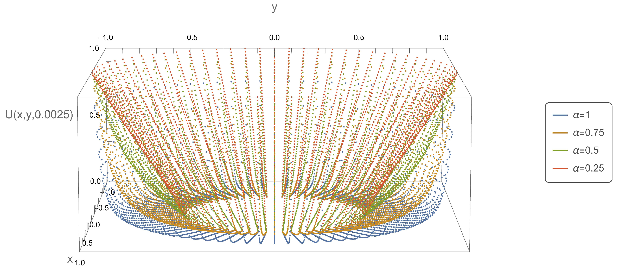
Figure 5, Figure 6, Figure 7 and Figure 8, present the axial symmetry of solution of the subdiffusion Equation (10) in the Cartesian coordinate system. Figure 1 and Figure 5, Figure 2 and Figure 6, etc. should be interpreted together, as they have been created based on the solution determined for the same time variable value. The figure with a higher number depicts the complete solution, while the figure with a lower number presents a segment of the complete solution for a fixed value of the variable $\varphi$. The values of the variable $\varphi$ were determined as follows: $\varphi =\frac{\pi i}{36}$, $i=1,2,\cdots ,72$. The x, y coordinates were determined using the relationship $x=rcos\varphi$, $y=rsin\varphi$.

In order to validate the numerical method proposed in Section 3.1, the results obtained with it were compared with those received by the inverse Laplace transform of the image (41) using the Gaver–Wynn–Rho algorithm implemented in Wolfram Mathematica. The comparison was made at twenty points $(r,t)\in \{0.6,0.7,0.8,0.9\}\times \{0.2,0.4,0.6,0.8,1\}$, which are common to all tested mesh variants.

Table 1. The value of $〈|U(r,t)-U^{GWR}(r,t)|〉$ for $\alpha =1$.

	$\mathbf{\Delta }\mathit{r}$	$\frac{1}{50}$	$\frac{1}{100}$	$\frac{1}{200}$	$\frac{1}{400}$
$\mathbf{\Delta }\mathit{t}$
$\frac{1}{50}$		2.394 × 10${}^{-}$${}^4$	2.538 × 10${}^{-}$${}^4$	2.581 × 10${}^{-}$${}^4$	2.592 × 10${}^{-}$${}^4$
$\frac{1}{100}$		2.162 × 10${}^{-}$${}^5$	1.897 × 10${}^{-}$${}^5$	1.863 × 10${}^{-}$${}^5$	1.855 × 10${}^{-}$${}^5$
$\frac{1}{200}$		1.404 × 10${}^{-}$${}^5$	7.29 × 10${}^{-}$${}^6$	5.843 × 10${}^{-}$${}^6$	5.491 × 10${}^{-}$${}^6$
$\frac{1}{400}$		1.189 × 10${}^{-}$${}^5$	4.56 × 10${}^{-}$${}^6$	2.733 × 10${}^{-}$${}^6$	2.278 × 10${}^{-}$${}^6$

,

Table 2. The value of $〈|U(r,t)-U^{GWR}(r,t)|〉$ for $\alpha =0.75$.

	$\mathbf{\Delta }\mathit{r}$	$\frac{1}{50}$	$\frac{1}{100}$	$\frac{1}{200}$	$\frac{1}{400}$
$\mathbf{\Delta }\mathit{t}$
$\frac{1}{50}$		1.943 × 10${}^{-}$${}^4$	1.873 × 10${}^{-}$${}^4$	1.855 × 10${}^{-}$${}^4$	1.851 × 10${}^{-}$${}^4$
$\frac{1}{100}$		1.026 × 10${}^{-}$${}^4$	9.565 × 10${}^{-}$${}^5$	9.39 × 10${}^{-}$${}^5$	9.346 × 10${}^{-}$${}^5$
$\frac{1}{200}$		5.609 × 10${}^{-}$${}^5$	4.91 × 10${}^{-}$${}^5$	4.734 × 10${}^{-}$${}^5$	4.691 × 10${}^{-}$${}^5$
$\frac{1}{400}$		3.273 × 10${}^{-}$${}^5$	2.574 × 10${}^{-}$${}^5$	2.399 × 10${}^{-}$${}^5$	2.355 × 10${}^{-}$${}^5$

,

Table 3. The value of $〈|U(r,t)-U^{GWR}(r,t)|〉$ for $\alpha =0.5$.

	$\mathbf{\Delta }\mathit{r}$	$\frac{1}{50}$	$\frac{1}{100}$	$\frac{1}{200}$	$\frac{1}{400}$
$\mathbf{\Delta }\mathit{t}$
$\frac{1}{50}$		1.71 × 10${}^{-}$${}^4$	1.647 × 10${}^{-}$${}^4$	1.632 × 10${}^{-}$${}^4$	1.628 × 10${}^{-}$${}^4$
$\frac{1}{100}$		8.98 × 10${}^{-}$${}^5$	8.352 × 10${}^{-}$${}^5$	8.195 × 10${}^{-}$${}^5$	8.156 × 10${}^{-}$${}^5$
$\frac{1}{200}$		4.91 × 10${}^{-}$${}^5$	4.282 × 10${}^{-}$${}^5$	4.125 × 10${}^{-}$${}^5$	4.085 × 10${}^{-}$${}^5$
$\frac{1}{400}$		2.874 × 10${}^{-}$${}^5$	2.246 × 10${}^{-}$${}^5$	2.089 × 10${}^{-}$${}^5$	2.049 × 10${}^{-}$${}^5$

and

Table 4. The value of $〈|U(r,t)-U^{GWR}(r,t)|〉$ for $\alpha =0.25$.

	$\mathbf{\Delta }\mathit{r}$	$\frac{1}{50}$	$\frac{1}{100}$	$\frac{1}{200}$	$\frac{1}{400}$
$\mathbf{\Delta }\mathit{t}$
$\frac{1}{50}$		9.345 × 10${}^{-}$${}^5$	8.755 × 10${}^{-}$${}^5$	8.607 × 10${}^{-}$${}^5$	8.57 × 10${}^{-}$${}^5$
$\frac{1}{100}$		5.052 × 10${}^{-}$${}^5$	4.461 × 10${}^{-}$${}^5$	4.313 × 10${}^{-}$${}^5$	4.276 × 10${}^{-}$${}^5$
$\frac{1}{200}$		2.917 × 10${}^{-}$${}^5$	2.326 × 10${}^{-}$${}^5$	2.178 × 10${}^{-}$${}^5$	2.141 × 10${}^{-}$${}^5$
$\frac{1}{400}$		1.852 × 10${}^{-}$${}^5$	1.261 × 10${}^{-}$${}^5$	1.113 × 10${}^{-}$${}^5$	1.076 × 10${}^{-}$${}^5$

collect the average absolute difference between the solution obtained via the proposed numerical method $U(r,t)$ and that obtained via the inverse Laplace transform $U^{GWR}(r,t)$. The analysis of all the tables leads to the observation that as the steps of the grid $\Delta r$ and $\Delta t$ are reduced, $U(r,t)$ then converges to $U^{GWR}(r,t)$ for all tested values of the order $\alpha$.

5. Convergence Analysis

The order of convergence of the proposed numerical scheme was estimated using EOC (experimental order of the convergence) and calculated as follows [37]:

$$EOC={log}_2\frac{〈|U_{i,j}^{\frac{1}{1600},\frac{1}{1600}}-U_{i,j}^{\Delta t,\Delta r}|〉}{〈|U_{i,j}^{\frac{1}{1600},\frac{1}{1600}}-U_{i,j}^{\Delta t/2,\Delta r/2}|〉}={log}_2\left(\frac{\Delta U^{\Delta t,\Delta r}}{\Delta U^{\Delta t/2,\Delta r/2}}\right),$$

(45)

where by $U_{i,j}^{\Delta t,\Delta r}$ denoted the numerical solution of the considered equation at nodal points common to all considered meshes $(\frac{1}{2}+\frac{i}{50},\frac{j}{50})$ for $i=0,...,25$, $j=0,...,50$, with time step $\Delta t\in \left\{\frac{1}{50},\frac{1}{100},\frac{1}{200}\right\}$ and spatial step $\Delta r\in \left\{\frac{1}{50},\frac{1}{100},\frac{1}{200}\right\}$. The reference numerical solution obtained under the fine mesh is denoted by $U_{i,j}^{\frac{1}{1600},\frac{1}{1600}}$. We use the Formula (45) only when the closed analytical solution is not available. The calculation results shown in

Table 5. Convergence order of the proposed numerical scheme for $\alpha \in \{1,0.75\}$.

				$\mathit{\alpha }$ = 1		$\mathit{\alpha }$ = 0.75
$\mathit{n}$	$\mathit{m}$	$\mathbf{\Delta }\mathit{t}$	$\mathbf{\Delta }\mathit{r}$	$\mathbf{\Delta }{\mathit{U}}^{\mathbf{\Delta }\mathit{t},\mathbf{\Delta }\mathit{r}}$	EOC	$\mathbf{\Delta }{\mathit{U}}^{\mathbf{\Delta }\mathit{t},\mathbf{\Delta }\mathit{r}}$	EOC
50	25	$\frac{1}{50}$	$\frac{1}{50}$	4.721 × 10${}^{-}$${}^3$	-	2.759 × 10${}^{-}$${}^3$	-
100	50	$\frac{1}{100}$	$\frac{1}{100}$	1.781 × 10${}^{-}$${}^3$	1.406	6.509 × 10${}^{-}$${}^4$	2.084
200	100	$\frac{1}{200}$	$\frac{1}{200}$	7.416 × 10${}^{-}$${}^4$	1.264	2.857 × 10${}^{-}$${}^4$	1.188
400	200	$\frac{1}{400}$	$\frac{1}{400}$	2.939 × 10${}^{-}$${}^4$	1.3353	1.231 × 10${}^{-}$${}^4$	1.215

and

Table 6. Convergence order of the proposed numerical scheme for $\alpha \in \{0.5,0.25\}$.

				$\mathit{\alpha }$ = 0.5		$\mathit{\alpha }$ = 0.25
$\mathit{n}$	$\mathit{m}$	$\mathbf{\Delta }\mathit{t}$	$\mathbf{\Delta }\mathit{r}$	$\mathbf{\Delta }{\mathit{U}}^{\mathbf{\Delta }\mathit{t},\mathbf{\Delta }\mathit{r}}$	EOC	$\mathbf{\Delta }{\mathit{U}}^{\mathbf{\Delta }\mathit{t},\mathbf{\Delta }\mathit{r}}$	EOC
50	25	$\frac{1}{50}$	$\frac{1}{50}$	1.15 × 10${}^{-}$${}^3$	-	2.836 × 10${}^{-}$${}^4$	-
100	50	$\frac{1}{100}$	$\frac{1}{100}$	1.788 × 10${}^{-}$${}^4$	2.684	7.505 × 10${}^{-}$${}^5$	1.918
200	100	$\frac{1}{200}$	$\frac{1}{200}$	1.117 × 10${}^{-}$${}^4$	0.679	4.03 × 10${}^{-}$${}^5$	0.897
400	200	$\frac{1}{400}$	$\frac{1}{400}$	4.913 × 10${}^{-}$${}^5$	1.186	1.715 × 10${}^{-}$${}^5$	1.233

indicate that the order of convergence of the proposed method is approximately equal to one.

The results presented at the end of the last section clearly show that the solutions obtained with the Gaver–Wynn–Rho algorithm are more accurate than those obtained with the generalized Crank–Nicolson method. Thus, we can use the following formula to estimate the experimental order of convergence:

$$EOC={log}_2\frac{〈|U_{i,j}^{GWR}-U_{i,j}^{\Delta t,\Delta r}|〉}{〈|U_{i,j}^{GWR}-U_{i,j}^{\Delta t/2,\Delta r/2}|〉}={log}_2\left(\frac{\Delta U^{\Delta t,\Delta r}}{\Delta U^{\Delta t/2,\Delta r/2}}\right),$$

(46)

where $U_{i,j}^{GWR}$ is a good approximation of the exact solution at the corresponding grid nodes.

The contents of

Table 7. Convergence order of the proposed numerical scheme for $\alpha \in \{1,0.75\}$.

				$\mathit{\alpha }$ = 1		$\mathit{\alpha }$ = 0.75
$\mathit{n}$	$\mathit{m}$	$\mathbf{\Delta }\mathit{t}$	$\mathbf{\Delta }\mathit{r}$	$\mathbf{\Delta }{\mathit{U}}^{\mathbf{\Delta }\mathit{t},\mathbf{\Delta }\mathit{r}}$	EOC	$\mathbf{\Delta }{\mathit{U}}^{\mathbf{\Delta }\mathit{t},\mathbf{\Delta }\mathit{r}}$	EOC
50	25	$\frac{1}{50}$	$\frac{1}{50}$	2.394 × 10${}^{-}$${}^4$	-	1.943 × 10${}^{-}$${}^4$	-
100	50	$\frac{1}{100}$	$\frac{1}{100}$	1.897 × 10${}^{-}$${}^5$	3.658	9.565 × 10${}^{-}$${}^5$	1.022
200	100	$\frac{1}{200}$	$\frac{1}{200}$	5.843 × 10${}^{-}$${}^6$	1.699	4.734 × 10${}^{-}$${}^5$	1.015
400	200	$\frac{1}{400}$	$\frac{1}{400}$	2.278 × 10${}^{-}$${}^6$	1.359	2.355 × 10${}^{-}$${}^5$	1.007

and

Table 8. Convergence order of the proposed numerical scheme for $\alpha \in \{0.5,0.25\}$.

				$\mathit{\alpha }$ = 0.5		$\mathit{\alpha }$ = 0.25
$\mathit{n}$	$\mathit{m}$	$\mathbf{\Delta }\mathit{t}$	$\mathbf{\Delta }\mathit{r}$	$\mathbf{\Delta }{\mathit{U}}^{\Delta \mathit{t},\Delta \mathit{r}}$	EOC	$\mathbf{\Delta }{\mathit{U}}^{\mathbf{\Delta }\mathit{t},\mathbf{\Delta }\mathit{r}}$	EOC
50	25	$\frac{1}{50}$	$\frac{1}{50}$	1.71 × 10${}^{-}$${}^4$	-	9.345 × 10${}^{-}$${}^5$	-
100	50	$\frac{1}{100}$	$\frac{1}{100}$	8.352 × 10${}^{-}$${}^5$	1.034	4.461 × 10${}^{-}$${}^5$	1.067
200	100	$\frac{1}{200}$	$\frac{1}{200}$	4.125 × 10${}^{-}$${}^5$	1.018	2.178 × 10${}^{-}$${}^5$	1.034
400	200	$\frac{1}{400}$	$\frac{1}{400}$	2.049 × 10${}^{-}$${}^5$	1.009	1.076 × 10${}^{-}$${}^5$	1.017

clearly show that the experimental order of convergence tends to zero very quickly (except for $\alpha =1$, where the observed trend is slower) as the time and spatial step of the mesh decreases. These results are a direct consequence of the fact that the solution obtained with the Gaver–Wynn–Rho algorithm is more accurate than the reference numerical solution obtained for the steps $\Delta r=\Delta t=\frac{1}{1600}$.

6. Conclusions

The method proposed in the article is a generalization of the fractional Crank–Nicolson method to a two-dimensional subdiffusion equation in the polar coordinate system, taking into account the assumed symmetry of the area and boundary conditions. To validate the method, the obtained results were compared with those received using the semi-analytical approach, where the analytical solution in the Laplace transform domain was numerically inverted. It was observed that the method based on the discretization of the integro-differential equation generates solutions that converge to those obtained by the Gaver–Wynn–Rho algorithm. As the time and space steps are decreased, the average absolute difference between the solutions decreases. The fully numerical approach seems to be better, despite the lower accuracy of the generated solutions, due to the greater universality of the method. In the semi-analytical approach, each change in the boundary or initial conditions results in the need to determine a new solution, which is time consuming and, in some cases, problematic.

In the schedule of further research, it is planned to further study the convergence analysis of the proposed scheme and reduce its computational costs.

References

- Metzler, R.; Klafter, J. The random walk’s guide to anomalous diffusion: A fractional dynamics approach. Phys. Rep. 2000, 339, 1–77. [Google Scholar] [CrossRef]
- Metzler, R.; Klafter, J. The restaurant at the end of the random walk: Recent developments in the description of anomalous transport by fractional dynamics. J. Phys. A Math. Gen. 2004, 37, 161–208. [Google Scholar] [CrossRef]
- Weeks, E.; Urbach, J.; Swinney, L. Anomalous diffusion in asymmetric random walks with a quasi-geostrophic flow example. Phys. D Nonlinear Phenom. 1996, 97, 291–310. [Google Scholar] [CrossRef]
- Solomon, T.; Weeks, E.; Swinney, H. Observations of anomalous diffusion and Lévy flights in a 2-dimensional rotating flow. Phys. Rev. Lett. 1993, 71, 3975–3979. [Google Scholar] [CrossRef] [PubMed]
- Humphries, N.E.; Queiroz, N.; Dyer, J.R.M.; Pade, N.G.; Musyl, M.K.; Schaefer, K.M.; Fuller, D.W.; Brunnschweiler, J.M.; Doyle, T.K.; Houghton, J.D.R.; et al. Environmental context explains Lévy and Brownian movement patterns of marine predators. Nature 2010, 465, 1066–1069. [Google Scholar] [CrossRef]
- Kosztołowicz, T.; Dworecki, K.; Mrówczyński, S. How to Measure Subdiffusion Parameters. Phys. Rev. Lett. 2005, 94, 170602. [Google Scholar] [CrossRef]
- Kosztołowicz, T.; Dworecki, K.; Mrówczyński, S. Measuring subdiffusion parameters. Phys. Rev. E 2005, 71, 041105. [Google Scholar] [CrossRef]
- Brociek, R.; Słota, D.; Król, M.; Matula, G.; Kwaśny, W. Comparison of mathematical models with fractional derivative for the heat conduction inverse problem based on the measurements of temperature in porous aluminum. Int. J. Heat Mass Transf. 2019, 143, 118440. [Google Scholar] [CrossRef]
- Li, X.C. Fractional Moving Boundary Problems and Some of Its Applications to Controlled Release System of Drug. Ph.D. Thesis, Shandong University, Jinan, China, 2009. [Google Scholar]
- Yin, C.; Li, X. Anomalous diffusion of drug release from slab matrix: Fractional diffusion models. Int. J. Pharm. 2011, 418, 78–87. [Google Scholar] [CrossRef]
- Voller, V.R. An exact solution of a limit case Stefan problem governed by a fractional diffusion equation. Int. J. Heat Mass Transf. 2010, 53, 5622–5625. [Google Scholar] [CrossRef]
- Voller, V.R. Fractional Stefan problems. Int. J. Heat Mass Transf. 2014, 74, 269–277. [Google Scholar] [CrossRef]
- Chmielowska, A.; Słota, D. Fractional Stefan Problem Solving by the Alternating Phase Truncation Method. Symmetry 2022, 14, 2287. [Google Scholar] [CrossRef]
- Błasik, M.; Klimek, M. Numerical solution of the one phase 1D fractional Stefan problem using the front fixing method. Math. Methods Appl. Sci. 2015, 38, 3214–3228. [Google Scholar] [CrossRef]
- Roscani, S.; Marcus, E. Two equivalent Stefans problems for the time fractional diffusion equation. Fract. Calc. Appl. Anal. 2013, 16, 802–815. [Google Scholar] [CrossRef]
- Roscani, S. Hopf lemma for the fractional diffusion operator and its application to a fractional free-boundary problem. J. Math. Anal. Appl. 2015, 434, 125–135. [Google Scholar] [CrossRef]
- Błasik, M. A Numerical Method for the Solution of the Two-Phase Fractional Lamé–Clapeyron–Stefan Problem. Mathematics 2020, 8, 2157. [Google Scholar] [CrossRef]
- Povstenko, Y.Z.; Kyrylych, T. Time-Fractional Heat Conduction in a Plane with Two External Half-Infinite Line Slits under Heat Flux Loading. Symmetry 2019, 11, 689. [Google Scholar] [CrossRef]
- Povstenko, Y.Z.; Klekot, J. Time-Fractional Heat Conduction in Two Joint Half-Planes. Symmetry 2019, 11, 800. [Google Scholar] [CrossRef]
- Povstenko, Y.Z. Linear Fractional Diffusion-Wave Equation for Scientists and Engineers; Springer International Publishing: Cham, Switzerland, 2015. [Google Scholar]
- Valkó, P.P.; Abate, J. Comparison of sequence accelerators forthe Gaver method of numerical Laplace transform inversion. Comput. Math. Appl. 2004, 48, 629–636. [Google Scholar] [CrossRef]
- Abate, J.; Valkó, P.P. Multi-precision Laplace transform inversion. Int. J. Numer. Methods Eng. 2004, 60, 979–993. [Google Scholar] [CrossRef]
- Guo, S.; Fan, X.; Gao, K.; Li, H. Precision controllable Gaver-Wynn-Rho algorithm in Laplace transform triple reciprocity boundary element method for three dimensional transient heat conduction problems. Eng. Anal. Bound. Elem. 2020, 114, 166–177. [Google Scholar] [CrossRef]
- Kang, Y.M. Simulating transient dynamics of the time-dependent time fractional Fokker–Planck systems. Phys. Lett. A 2016, 380, 3160–3166. [Google Scholar] [CrossRef]
- Kang, Y.M.; Jiang, Y.L.; Yong, X. Linear response characteristics of time-dependent time fractional Fokker–Planck equation systems. J. Phys. A Math. Theor. 2014, 47, 455005. [Google Scholar] [CrossRef]
- Ciesielski, M. Frakcjalna Metoda Roznic Skonczonych w Zastosowaniu do Modelowania Anomalnej Dyfuzji w Obszarze Ograniczonym. Ph.D. Thesis, Czestochowa University of Technology, Czestochowa, Poland, 2005. [Google Scholar]
- Liu, F.; Yang, C.; Burrage, K. Numerical method and analytical technique of the modified anomalous subdiffusion equation with a nonlinear source term. J. Comput. Appl. Math. 2009, 231, 160–176. [Google Scholar] [CrossRef]
- Zhuang, P.; Liu, F.; Anh, V.; Turner, I. New Solution and Analytical Techniques of the Implicit Numerical Method for the Anomalous Subdiffusion Equation. SIAM J. Numer. Anal. 2008, 46, 1079–1095. [Google Scholar] [CrossRef]
- Bhrawy, A.H.; Baleanu, D.; Mallawi, F. A new numerical technique for solving fractional sub-diffusion and reaction sub-diffusion equations with a non-linear source term. Therm. Sci. 2015, 19, 25–34. [Google Scholar] [CrossRef]
- Błasik, M. A Generalized Crank-Nicolson Method for the Solution of the Subdiffusion Equation. In Proceedings of the 23rd International Conference on Methods & Models in Automation & Robotics (MMAR), Międzyzdroje, Poland, 27–30 August 2018; pp. 726–729. [Google Scholar]
- Błasik, M. The implicit numerical method for the one-dimensional anomalous subdiffusion equation with a nonlinear source term. Bull. Pol. Acad. Sci. Tech. Sci. 2021, 69, e138240. [Google Scholar] [CrossRef]
- Błasik, M. Numerical methodfor the solution of the one-dimensional anomalous subdiffusion equation with a variable diffusion coefficient. Acta Phys. Pol. A 2020, 138, 228–231. [Google Scholar] [CrossRef]
- Zhang, P.; Pu, H. The error analysis of Crank-Nicolson-type difference scheme for fractional subdiffusion equation with spatially variable coefficient. Bound. Value Probl. 2017, 2017, 1–19. [Google Scholar] [CrossRef]
- Onal, M.; Esen, A. A Crank-Nicolson Approximation for the time Fractional Burgers Equation. Appl. Math. Nonlinear Sci. 2020, 5, 177–184. [Google Scholar] [CrossRef]
- Jin, B.; Li, B.; Zhou, Z. An analysis of the Crank–Nicolson method for subdiffusion. IMA J. Numer. Anal. 2017, 38, 518–541. [Google Scholar] [CrossRef]
- Wang, L.; Stynes, M. An α-robust finite difference method for a time-fractional radially symmetric diffusion problem. Comput. Math. Appl. 2021, 97, 386–393. [Google Scholar] [CrossRef]
- Gu, X.M.; Sun, H.W.; Zhao, Y.L.; Zheng, X. An implicit difference scheme for time-fractional diffusion equations with a time-invariant type variable order. Appl. Math. Lett. 2021, 120, 107270. [Google Scholar] [CrossRef]
- Luo, W.H.; Huang, T.Z.; Wu, G.C.; Gu, X.M. Quadratic spline collocation method for the time fractional subdiffusion equation. Appl. Math. Comput. 2016, 276, 252–265. [Google Scholar] [CrossRef]
- Luo, W.H.; Li, C.; Huang, T.Z.; Gu, X.M.; Wu, G.C. A High-Order Accurate Numerical Scheme for the Caputo Derivative with Applications to Fractional Diffusion Problems. Numer. Funct. Anal. Optim. 2017, 39, 600–622. [Google Scholar] [CrossRef]
- Yang, X.; Wu, L.; Zhang, H. A space-time spectral order sinc-collocation method for the fourth-order nonlocal heat model arising in viscoelasticity. Appl. Math. Comput. 2023, 457, 128192. [Google Scholar] [CrossRef]
- Chen, C.M.; Liu, F.; Turner, I.; Anh, V. Numerical schemes and multivariate extrapolation of a two-dimensional anomalous sub-diffusion equation. Numer. Algorithms 2010, 54, 1–21. [Google Scholar] [CrossRef]
- Sweilam, N.H.; Ahmed, S.M.; Adel, M. A simple numerical method for two-dimensional nonlinear fractional anomalous sub-diffusion equations. Math. Methods Appl. Sci. 2020, 44, 2914–2933. [Google Scholar] [CrossRef]
- Huang, H.; Cao, X. Numerical method for two dimensional fractional reaction subdiffusion equation. Eur. Phys. J. Spec. Top. 2013, 222, 1961–1973. [Google Scholar] [CrossRef]
- Yu, B.; Jiang, X.; Xu, H. A novel compact numerical method for solving the two-dimensional non-linear fractional reaction-subdiffusion equation. Numer. Algorithms 2015, 68, 923–950. [Google Scholar] [CrossRef]
- Aslefallah, M.; Shivanian, E. Nonlinear fractional integro-differential reaction-diffusion equation via radial basis functions. Eur. Phys. J. Plus 2015, 130. [Google Scholar] [CrossRef]
- Aslefallah, M.; Abbasbandy, S.; Shivanian, E. Numerical solution of a modified anomalous diffusion equation with nonlinear source term through meshless singular boundary method. Eng. Anal. Bound. Elem. 2019, 107, 198–207. [Google Scholar] [CrossRef]
- Yüzbaşı, Ş. Numerical solutions of fractional Riccati type differential equations by means of the Bernstein polynomials. Appl. Math. Comput. 2013, 219, 6328–6343. [Google Scholar] [CrossRef]
- Oloniiju, S.D.; Goqo, S.P.; Sibanda, P. A Chebyshev pseudo-spectral method for the multi-dimensional fractional Rayleigh problem for a generalized Maxwell fluid with Robin boundary conditions. Appl. Numer. Math. 2020, 152, 253–266. [Google Scholar] [CrossRef]
- Oloniiju, S.D.; Goqo, S.P.; Sibanda, P. A geometrically convergent pseudo-spectral method for multi-dimensional two-sided space fractional partial differential equations. J. Appl. Anal. Comput. 2021, 11, 1699–1717. [Google Scholar] [CrossRef] [PubMed]
- Kilbas, A.; Srivastava, H.; Trujillo, J. Theory and Applications of Fractional Differential Equations; Elsevier: Amsterdam, The Netherlands, 2006. [Google Scholar]
- Debnath, L.; Bhatta, D. Integral Transforms and Their Applications, 2nd ed.; Chapman and Hall: New York, NY, USA; CRC: New York, NY, USA, 2006. [Google Scholar]
- Podlubny, I. Fractional Differential Equations; Academic Press: San Diego, CA, USA, 1999. [Google Scholar]
- Zill, D.; Cullen, M. Differential Equations with Boundary-Value Problems; Cengage Learning: Boston, MA, USA, 2008. [Google Scholar]
- Barenblatt, G. Scaling, Self-Similarity, and Intermediate Asymptotics; Cambridge University Press: Cambridge, UK, 1996. [Google Scholar]
- Barenblatt, G. Scaling; Cambridge University Press: Cambridge, UK, 2003. [Google Scholar]
- Luchko, Y. Some uniqueness and existence results for the initial-boundary-value problems for the generalized time-fractional diffusion equation. Comput. Math. Appl. 2010, 59, 1766–1772. [Google Scholar] [CrossRef]
Figure 1.
Plot of determined numerically for and .
Figure 2.
Figure 3.
Figure 4.
Figure 5.
Plot of function determined numerically for .
Figure 6.
As in Figure 5, but for .
Figure 7.
Figure 8.