
Reliability Analysis of Kavya Manoharan Kumaraswamy Distribution under Generalized Progressive Hybrid Data


1
Department of Mathematical Sciences, College of Science, Princess Nourah bint Abdulrahman University, P.O. Box 84428, Riyadh 11671, Saudi Arabia
2
Department of Statistics, Faculty of Business Administration, Delta University for Science and Technology, Gamasa 11152, Egypt
3
Department of Mathematical Statistics, Faculty of Graduate Studies for Statistical Research, Cairo University, Cairo 12613, Egypt
4
Department of Statistics, Al-Azhar University, Cairo 11751, Egypt
*
Author to whom correspondence should be addressed.
Symmetry 2023, 15(9), 1671; https://0-doi-org.brum.beds.ac.uk/10.3390/sym15091671
Submission received: 25 July 2023
/
Revised: 19 August 2023
/
Accepted: 22 August 2023
/
Published: 30 August 2023
(This article belongs to the Special Issue Symmetrical and Asymmetrical Distributions in Statistics and Data Science)
Abstract
:Generalized progressive hybrid censoring approaches have been developed to reduce test time and cost. This paper investigates the difficulties associated with estimating the unobserved model parameters and the reliability time functions of the Kavya Manoharan Kumaraswamy (KMKu) distribution based on generalized type-II progressive hybrid censoring using classical and Bayesian estimation techniques. The frequentist estimators’ normal approximations are also used to construct the appropriate estimated confidence intervals for the unknown parameter model. Under symmetrical squared error loss, independent gamma conjugate priors are used to produce the Bayesian estimators. The Bayesian estimators and associated highest posterior density intervals cannot be derived analytically since the joint likelihood function is provided in a complicated form. However, they may be evaluated using Monte Carlo Markov chain (MCMC) techniques. Out of all the censoring choices, the best one is selected using four optimality criteria.
1. Introduction
The progressive type-II censoring (PCS-T2) method is the most popular scheme in reliability and survival analysis. Compared with the traditional type-II censoring method, it is better. Progressive censoring is advantageous in a variety of real-world applications, including business, medical research, and therapeutic settings. Up until the test’s conclusion, it permits the removal of any remaining experimental units. Assume that n units are used in a life test and that it is not desirable to record every failure because of financial and time constraints. Consequently, only a portion of unit failures are seen. A sample like this is known as a censored sample. Assume that one of the units was accidentally damaged after the test started but before they all burned out. This unit needs to be taken out of the life test if the experiment is still going on. In this situation, a framework for analyzing this kind of data is provided by the progressive censoring scheme. A few examples of primary references are [1,2].
PCS-T2 has drawn a lot of attention in the literature as a very flexible censoring system (see [3] for further details). When testing independent units at a time , the failure number to be noticed and the progressive censored samples, , where , are specified. When the initial failure is seen (suppose that ), the other surviving units are chosen at random, and of those units is disqualified from the test. Similarly, at the moment of the second failure (suppose that ), of are selected at random and deleted from the test, and so on. At the time of the failure (suppose that ), every survivor unit still present is removed from the experiment.
Whenever the test units are particularly reliable, the major drawback of this censoring is that it could take longer to finish the progressively type-II hybrid censored samples (PHCS-T2). The authors of [4] proposed a progressive type-I hybrid censored strategy (PHCS-T1) as a remedy for this issue. This method combines PCS-T2 with conventional type-I censoring. Under PHCS-T1, the trial period is stopped at , maximum likelihood estimators (MLEs) were not always available due to the fact that relatively a few failures might occur before time in PHCS-T1. To resolve this issue, [5] presented the PHCS-T2 scheme. At , the experiment comes to an end under PHCS-T2. It can take some time until such failures are really observed, despite the fact that PHCS-T2 promises a fixed number of failures.
It could take a while to gather the needed failures, even though the PHCS-T2 ensures an effective number of observable failures. Thus, [6] devised the generalized progressive type-II hybrid censoring (GPHC-T2). Assume that the thresholds and 2, as well as the integer , are preassigned in such a way that and . and represent the overall number of failures up to periods and, respectively. Then, at , of are arbitrarily excluded from the test, followed by of , and so on.
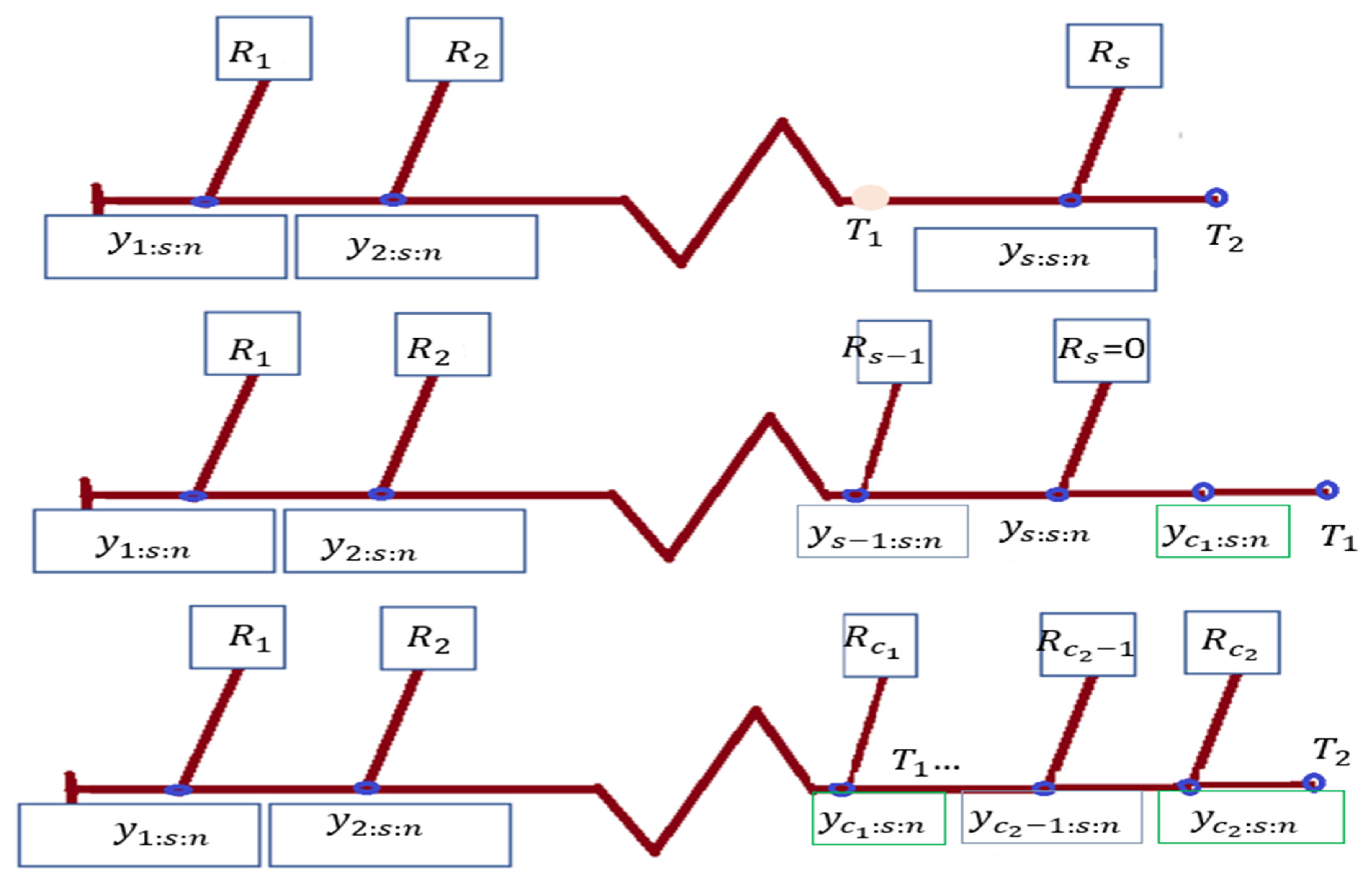
The experiment is over, and all remaining units are deleted at . If failures are observed without any further withdrawals up until time (Case-I); if , the test is terminated at time (Case-II); or, if not, the test is terminated at time (Case-III). Keep in mind that the GPHCS-T2 modifies the PHCS-T2 by guaranteeing that the test is completed at the scheduled time . demonstrates the longest period of time the researcher is willing to let the experiment continue. As a result, one of the following three data types will be visible to the experimenter:
Figure 1 indicates the cases of generalized type-II progressive hybrid sample as follows:
Assume that in a distribution with a cumulative distribution function (cdf) F(.), and probability density function (pdf) f(.), the variables and represent the respective lifetimes. As a result, the GPHCS-T2 likelihood function is expressed as follows:
where stand in for Case-I, Case-II, and Case-III, respectively, and is a combination form of dependability functions. Table 1 displays the GPHCS-T2 notations from Equation (1). Many censoring techniques can also be inferred as particular examples from Equation (1), including
- With setting to 0, use PHCS-T1.
- . by setting PHCS-T2.
- You may do hybrid type-I censoring by setting .
- , can be used to do hybrid type-II censoring.
- To do type-I censoring, set
- A type-II censored sample is produced by setting
On the basis of GPHCS-T2, more studies have been conducted. For instance, Ref. [7] investigated the prediction issue of forthcoming Burr-XII distribution failure rates. The authors of [8] created the Weibull distribution with little data with an objective Bayesian analysis. The authors of [9] addressed the competing risks from exponential data, and [10] more recently examined both the point and interval estimations of the Burr-XII parameters. Last but not least, [11] addressed the Fréchet distribution’s optimality under generalized censoring schemes. In this paper, the KMKu model under generalized censoring samples is studied. Where the KMKu model was initially proposed by [11]. Also, they found that the Kumaraswamy model’s and KMKu shape forms in the pdf for different parameter values are comparable. It may be asymmetric, unimodal, increasing, or decreasing. In addition, the bathtub, U-shape, J-shape, or increasing shapes of the hazard rate function (hrf) for the KMKu model are all possible. But suppose that is the lifespan random variable of a test item adheres to the KMKu distribution, denoted by the notation , where are the shape parameters. Therefore, it is supplied by its pdf, cdf, reliability function (RF), , and hrf, all represented by the letters , , and accordingly:
and
Although the KMKu model has a lot of flexibility because of its different shapes of hrf and pdf, to our knowledge, no studies have yet been done under censorship. Particularly, the generalized type-II progressively hybrid censoring scheme has not produced any data for the new KMKu lifetime model’s survival traits and model parameters. To fill this gap, the following are the objectives of this study: Firstly, the probability inference for any function of the unknown KMKu parameters, such as R(t) or h(t), is derived. The second objective is to derive independent gamma priors from the squared error (SE) loss and produce Bayes estimates for the same unknown parameters, employing the provided estimation procedures, such as classical and Bayesian approaches. The unknown parameters of the KMKu distribution are discovered using the approximation confidence intervals (ACIs) and highest posterior density (HPD) interval estimators. The acquired estimates are computed using the R programming language’s “maxLik” and “coda” packages because the theoretical findings of and obtained by the suggested estimation techniques cannot be represented in closed form. [12,13] offered these packages. Using four optimality criteria, the ultimate aim is to develop the most efficient progressively censored sample technique. The effectiveness of the different estimators is investigated using a Monte Carlo simulation with the entire sample size, which can be combined in a variety of ways, effective sample size, threshold timings, and progressively censored samples. We compare the average confidence lengths (ACLs), mean relative absolute biases (MRABs), and simulated root mean squared errors (RMSEs) of the derived estimators. The optimal censoring tactic should be chosen after evaluating how effectively the given techniques will function in practice. The remaining portions of this study are structured as follows: The maximum likelihood, Bayes inferences, and reliability functions of the unknown parameters are presented in Section 2 and Section 3, respectively. The credible and asymptotic intervals are built into Section 4. Section 5 goes into depth about the results of the Monte Carlo simulation. The optimal methods for progressive censoring are discussed in Section 6. Two actual data sets are indicated in Section 7. Finally, the conclusion and discussion are given in Section 8.
2. Likelihood Estimation
Assume that the representation of a GPHCS-T2 sample of size taken from is . The probability function of GPHCS-T2 may be represented by substituting for in Equation (1) and adding Equations (2) and (3); for more information, see [14].
where
and .
The proper log-likelihood function for Equation (6) is as follows:
where
, and
By partially differentiating Equation (7) with reference to and , the subsequent two findings are produced. After being equal to zero, likelihood equations must be simultaneously solved in order to create the MLEs.
and
where and , respectively, we have
,
According to Equations (8) and (9), it is necessary to simultaneously satisfy a system of two nonlinear equations in order to derive the MLEs of and in the KMKu model. As a result, for and , there is not, and cannot be computed, an analytical closed-form solution. Thus, it may be estimated for each specific GPHCS-T2 data set using numerical techniques like the Newton-Raphson iterative method. When the estimates of and are derived by replacing them with and , the MLEs and , respectively, may be easily computed.
3. Bayes Estimator
The HPD intervals for the Bayes estimators of , R(t), and h(t) are developed using the SE loss function. To do this, it is assumed that the KMKu parameters and , respectively, have independent gamma priors of the forms and .
The normal distribution can be a standard choice for data if the domain of that distribution is from −∞ to ∞, and the beta distribution can be a standard choice for data if the domain of that distribution is from 0 to 1. Similarly, the gamma distribution can be a standard choice for non-negative continuous data if the domain of the gamma distribution is from 0 to ∞. This is one of the most important reasons, but there are other reasons as follows:
- We believe the main motivation for the gamma prior is usually to constrain the random variables to positive values.
- The gamma distribution is considered one of the most important and well-known statistical distributions because it is compatible with many engineering, mathematical, statistical, and medical applications.
- The gamma distribution is one of the most famous distributions that is used in mathematical solutions (integrations), especially when the data are from 0 to ∞.
- In previous studies, the gamma distribution was the most popular prior distribution and was associated with the best statistical results.
Gamma priors should be considered for a variety of reasons, including the fact that they are (1) adjustable, (2) offer diverse shapes based on parameter values, and (3) fairly basic and brief and might not generate a solution to a challenging estimation problem. Then, the combined previous density of and is determined; for more details on this topic, see [15,16].
If it is anticipated that for are known. The joint posterior pdf of and Equations (6) and (10), when combined, results.
The Bayes estimate, , of and respectively, under SE loss, is what is meant by the posterior expectation of Equation (11), which is given.
It is clear from Equation (11), that it is impossible to explicitly express the marginal pdfs of and . In order to accomplish this, we recommend creating samples from Equation (11) utilizing Bayes MCMC methods to calculate the joint Bayes estimates and supplying their HPD intervals. The complete conditional pdfs of and are provided for the MCMC sampler from Equation (11) to be performed as intended.
and
The Metropolis-Hastings (M-H) approach is considered to be the best solution to this problem because no analytical method exists to reduce the posterior pdfs of and in Equations (12) and (13), respectively, to any known distribution (for further information, see [17,18]. The sampling method of the M-H algorithm is implemented according to:
First, establish the starting points, and .
Set S = 1 after that.
Thirdly, from and , respectively, create and .
The fourth step: Obtaining and
Fifth, use the uniform distribution to generate the samples and .
Sixth: Set and respectively, if and are both smaller than and , respectively. Set and , correspondingly, if not.
Seventh: Establish that S equals S + 1.
Eighth: Repeating steps three through seven a number of times will give you the values for and for .
Ninth: To calculate the RF in Equation (4) and hrf in Equation (5), use and for , respectively, for a given mission period .
and
The convergence of the MCMC sampler must be ensured, and starting, and values must be eliminated. The first simulated variants, let us say , are removed as burn-ins. Therefore, using the remaining samples of or , (let us suppose ), the Bayesian estimates are computed. On the basis of the SE loss function, the Bayes MCMC estimates of are shown.
4. Interval Estimators
The HPD interval estimators in this section are based on acquired MCMC-simulated variations, as opposed to the approximative confidence estimators of or that are based on observed Fisher information.
4.1. Asymptotic Intervals
To compute the ACIs for and , the Fisher information matrix must first be inverted to produce the asymptotic variance-covariance (AVC) matrix. According to certain regularity criteria, is nearly normal with a mean and variance . In agreement with [19], we estimate by , replacing and for and .
where
where
and
The two-sided ACIs are therefore given by
and for and , respectively, where stands for the top percentage points of the standard normal distribution, and are the primary diagonal elements of Equation (14). Furthermore, we employ the delta method to first establish the estimated variance of and (see [20]) before developing the ACIs of and as
where , and
Then, R(t) and h(t) both have two-sided ACIs that are supplied by and , respectively.
Adding bootstrapping techniques to improve estimators or create confidence intervals for , , or is easy.
4.2. HPD Intervals
The method put forward by [21] is used to create HPD interval estimates of , or . First, we assign numerical values to the MCMC samples of for correspondingly. The discovery is that the two-sided HPD interval of is supplied by , where is selected so that
5. Optimal PCS-T2 Designs
The experimenter may want to pick the “best” censoring scheme out of a collection of all accessible censoring schemes in order to provide the most details about the unknown parameters under investigation, especially in the context of dependability. First, [1] examined the problem of deciding which censoring strategy is most appropriate under various circumstances. However, a number of optimality criteria, , where have been proposed, and several assessments of the top censoring strategies have been made. The precise values of (total test units), (effective sample), and (ideal test thresholds) are picked in advance according to the accessibility of the units, the accessibility of the experimental settings, and cost factors (see [22]). A number of articles in the literature have addressed the topic of contrasting two (or more) different censoring techniques. For examples, see [23,24]. To help us choose the best censoring strategy, , Table 2 offers a variety of widely used measures.
It is advised that the observed Fisher information, values for , be maximized. For criterion and , we also wish to reduce the determinant and trace of . The best censoring strategy for multi-parameter distributions may be selected using scale-invariant criteria. While dealing with unknown multi-parameter distributions makes it more challenging to compare the two Fisher information matrices, dealing with single-parameter distributions allows for the use of scale-invariant criteria to compare a variety of criteria . The logarithmic MLE of the quantile, , tends to have a variance that is minimized by the p-dependent criterion . As a result, the logarithm of the KMKu distribution for time may be calculated using
By using the delta technique to solve for Equation (4), the estimate of the variance for the of the KMKu distribution is given as
where
while The maximum value of the criterion and the lowest value of correspond to the best censoring. On the other hand, the greatest value of the criterion and the lowest value of the criterion correspond to the best censoring.
6. Simulation
Using different combinations of (threshold points), n (sample size), s (size of censored sample), and R (censored removal), Monte-Carlo (MC) simulations were carried out to assess the true performance of the acquired point and interval estimators of and . To establish this goal, for KMKu(1.4, 1.5), KMKu(1.4, 0.5), and KMKu(0.4, 0.5), we replicated the GPHCS-T2 mechanism 1000 times. Taking , two different choices of n and s were used as (n = 30, 50, 100), and the choices of s were used as (s = 20, 25) at n = 30, (s = 35, 45) at n = 50, and (s = 70, 90) at n = 100. At = 0.6, the true values of and were 0.4278 and 1.4899, respectively. At = 0.85, the true values of and were 0.2526 and 3.3106, respectively.
Additionally, by utilizing the binomial elimination distribution and taking into account different censoring schemes for each combination of and , the following is conducted: according to the following probability mass function, the number of units removed at each failure time is expected to follow a binomial distribution.
Additionally, assume that for any , is independent of . In light of this, the likelihood function can be written as follows:
where
That is,
where the GPHCS-T2-based KMKu distribution’s parameters do not affect the binomial parameter (Independent). We chose the binomial parameter with varied values of 0.3 and 0.8.
The MLEs and 95% ACI estimates of and were assessed after 1000 GPHCS-T2 samples had been gathered using R 4.2.2 programming software and the “maxLik” library. We simulated 12,000 MCMC samples and omitted the first 2000 iterations as burn-in to obtain the Bayes point estimates along with their HPD interval estimates of the same unknown parameters using the “coda” library in the R 4.2.2 programming language. The estimates and their variances were equated with the Fisher information matrix of and to produce the ML estimator, which it denoted as elective hyper-parameters, and this was contributed by [25]. This process allowed for the extraction of the hyper-parameters of the informative priors.
- The key general finding is that the suggested values for and performed well.
- All estimations of R(t), and h(t) functioned satisfactorily as n(or s) grew.
- In most cases, the MSE, Bias, and WCI of all unknown parameters fell while their CPs grew as (T1, T2) increased.
- Due to the gamma information, the Bayes estimates of and behaved more predictably than the other estimates. Regarding credible HPD intervals, the same statement might be made.
- When the parameter of binomial r was increased, the proposed estimates of and performed better in most cases.
7. Application
The data set, which has been examined by [11], had 30 assessments of the tensile strength of polyester fibers. The following details are included in the data set: “0.023, 0.032, 0.054, 0.069, 0.081, 0.094, 0.105, 0.127, 0.148, 0.169, 0.188, 0.216, 0.255, 0.277, 0.311, 0.361, 0.376, 0.395, 0.432, 0.463, 0.481, 0.519, 0.529, 0.567, 0.642, 0.674, 0.752, 0.823, 0.887, 0.926”. For data on the strength of polyester fibers, where the Kolmogorov-Smirnov distance is 0.0569 with a p-value of 0.9999, [11] explores the MLE of this model using several measures of goodness-of-fit. The Kolmogorov-Smirnov test findings showed that the KMKu distribution fits the data on polyester fiber strength.
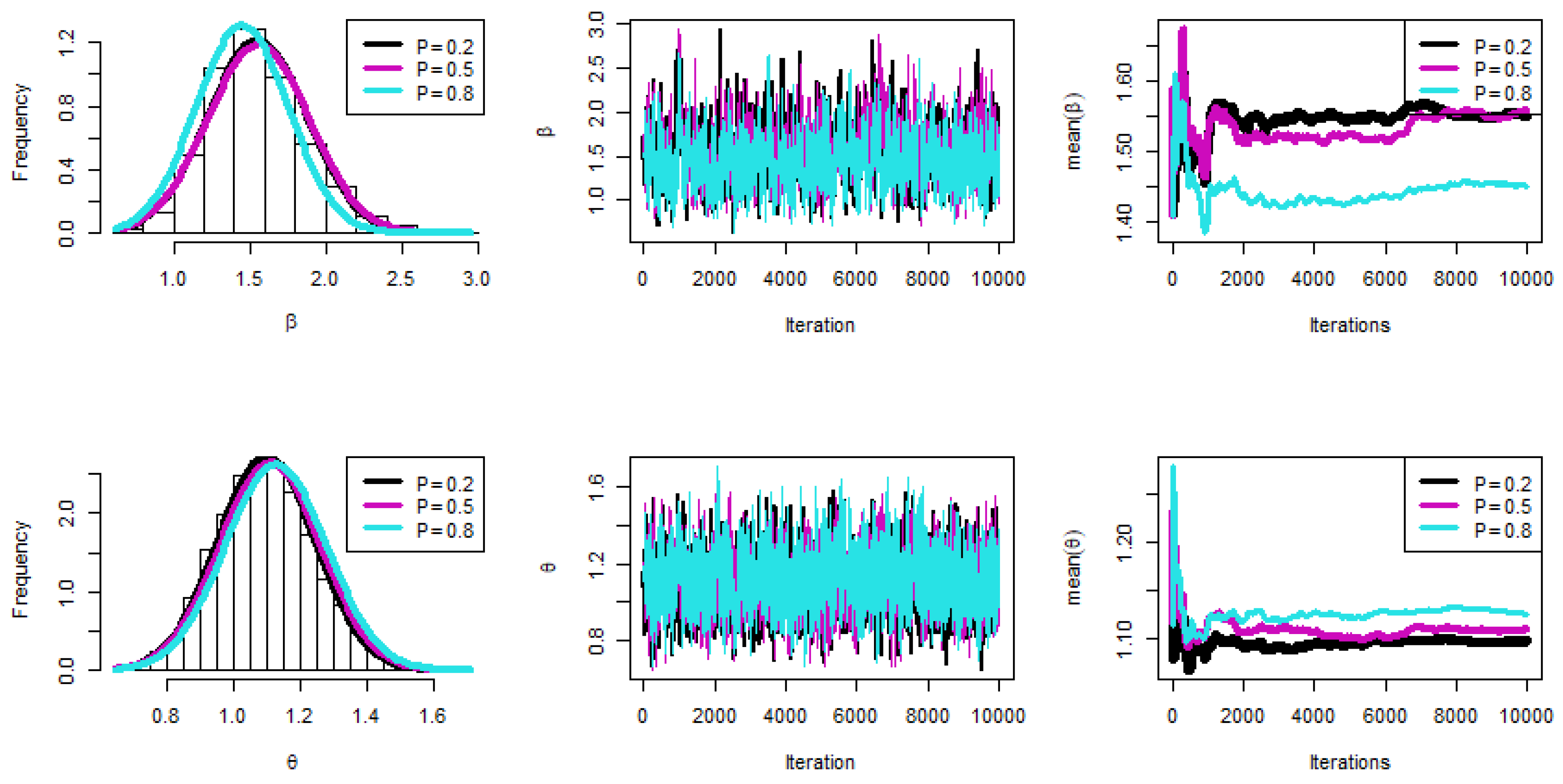
Two GPHCS-T2 samples with s = 20 and 25 were produced from the tensile strength of polyester fibers data in order to explain the proposed estimation methodology. The binomial removal has been used to obtain the GPHCS-T2 samples with different parameters of p = 0.2, 0.5, and 0.8. Table 6 lists the computed R(t) and h(t) at t = 0.6 and 0.85 by maximum likelihood estimates (MLE) and Bayesian estimation, respectively, along with their standard error (SE). By repeating the MCMC sampler 12,000 times and disregarding the first 2000 times as burn-in, the Bayes estimates (with their SE) were evaluated using incorrect gamma priors and are also provided in Table 4 because there was no prior knowledge about the unknown KMKu parameters and from the given data set. In order to estimate unknown hyperparameters for the computational logic, elective hyperparameters were employed. In terms of the minimum standard error and interval width values, it is evident from Table 6 that the MCMC estimates of and performed better than the others.
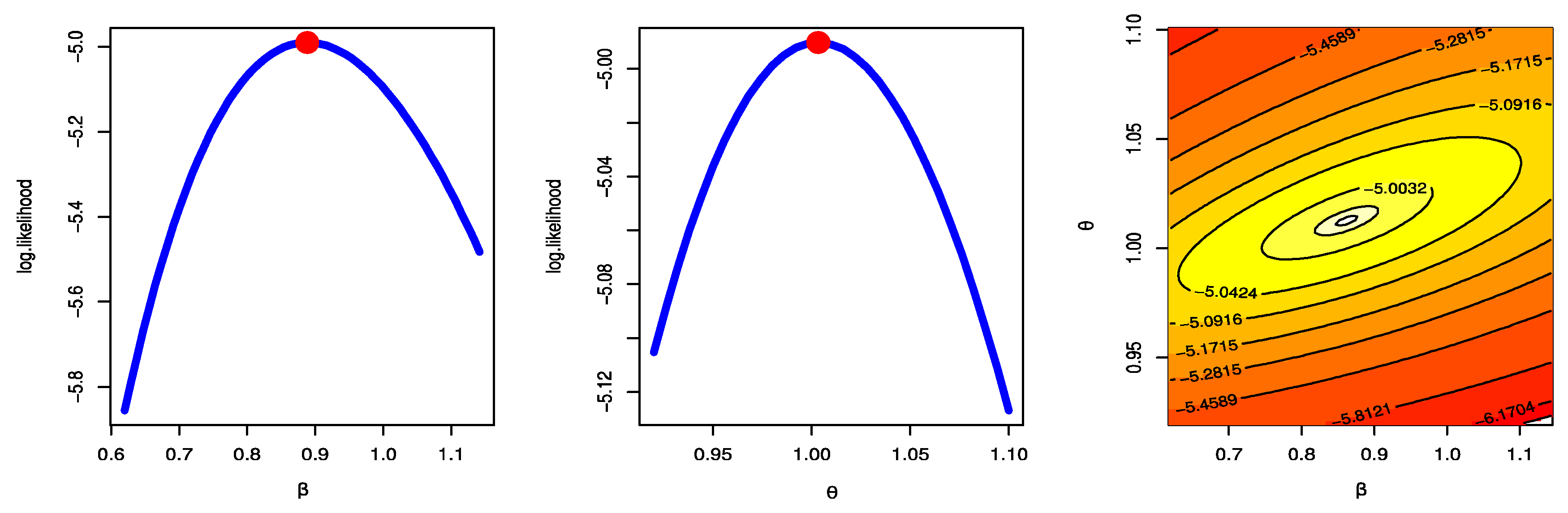
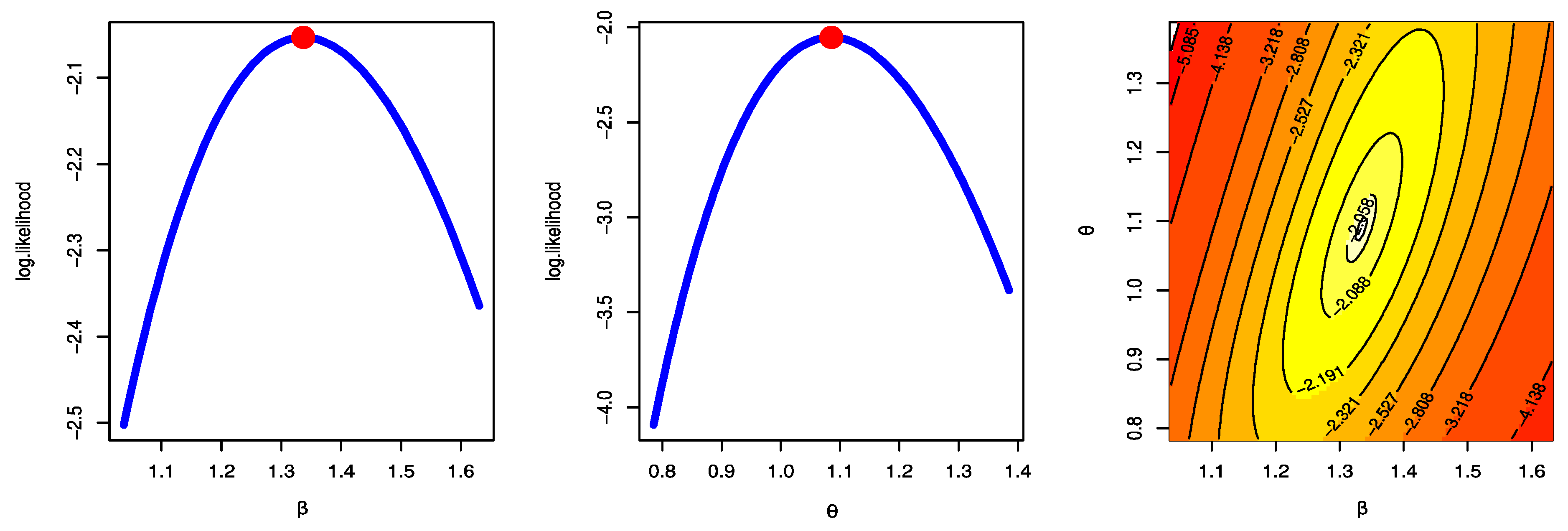
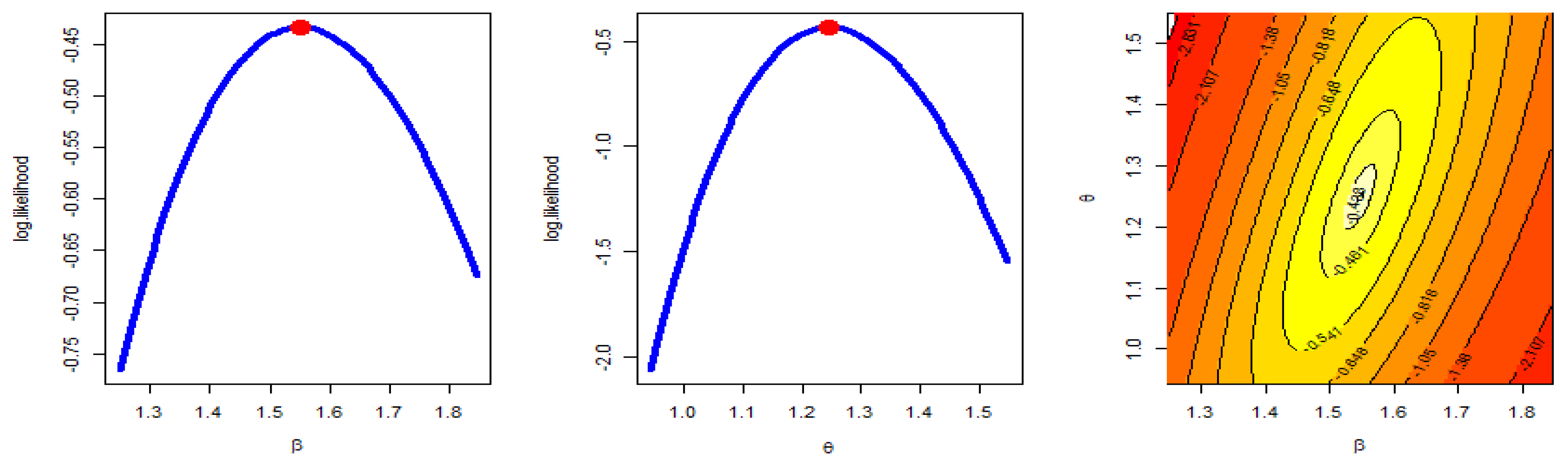
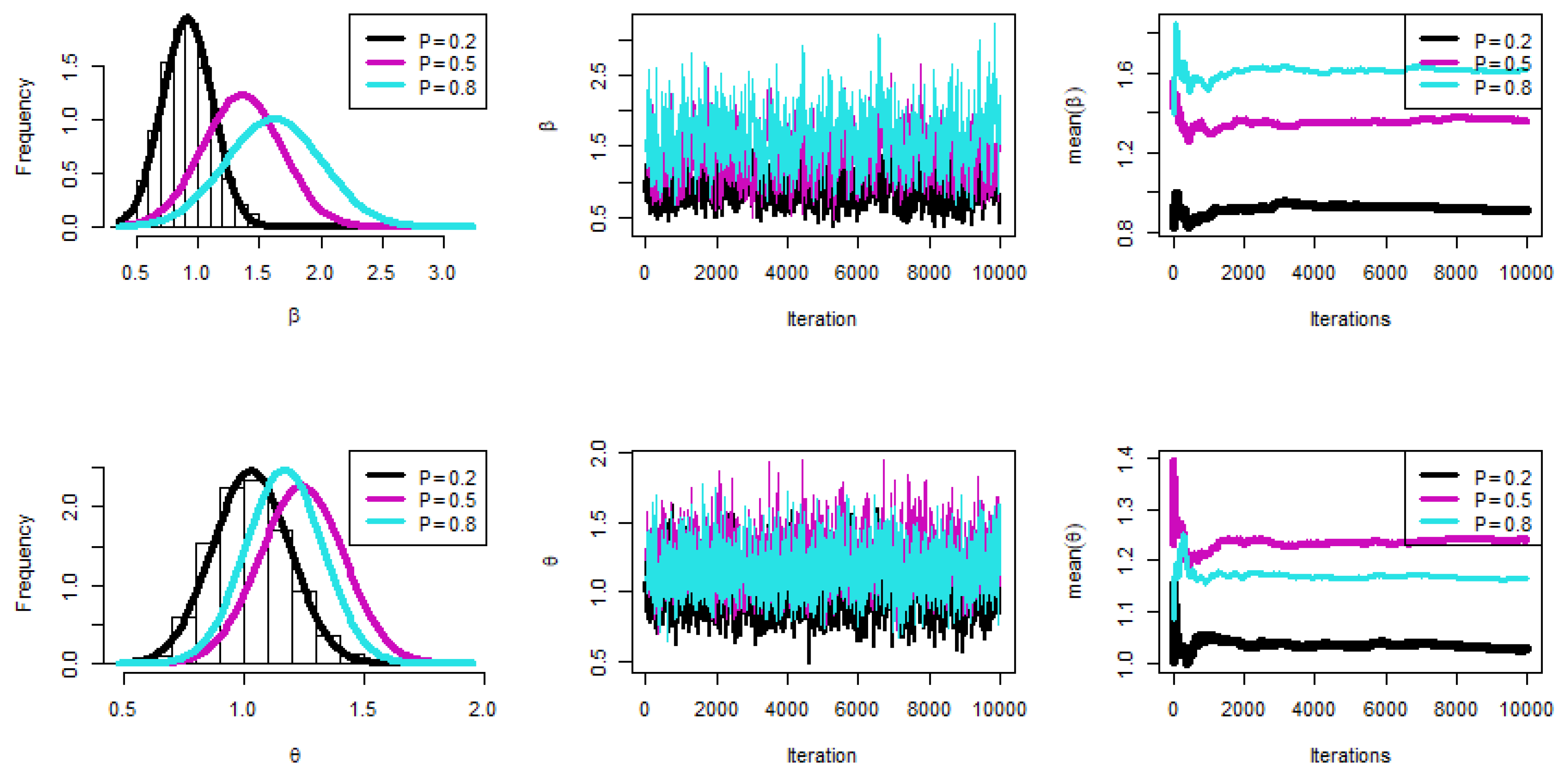
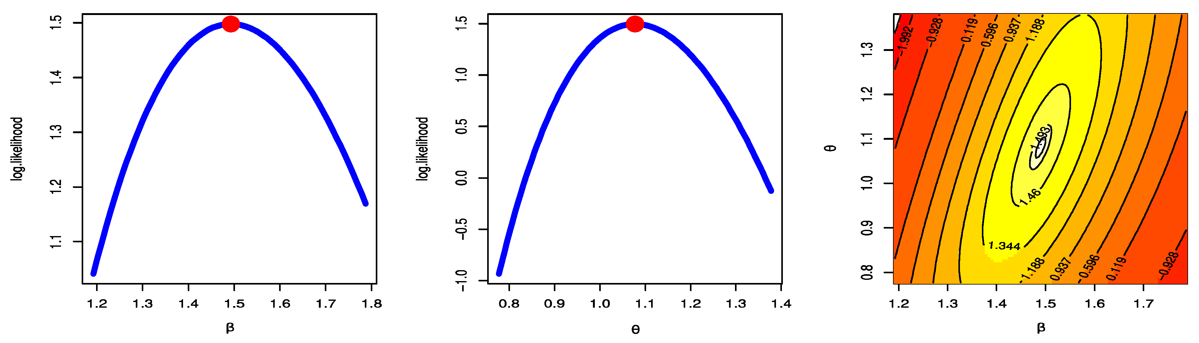
Figure 2, Figure 3 and Figure 4 were created to examine the maximum values of the estimators by profile likelihood as well as the existence and uniqueness of the log-likelihood function by contour plot with regard to different d and q options based on GPHCS-T2 samples with s = 20 and distinct p = 0.2, 0.5, and 0.8, respectively. Figure 5 clearly shows that the MCMC technique converged favorably and that the recommended size of the burn-in sample was adequate to completely nullify the impact of the recommended beginning values. Figure 5 demonstrates that the estimated estimates of and were roughly symmetrical for each sample when s = 20.
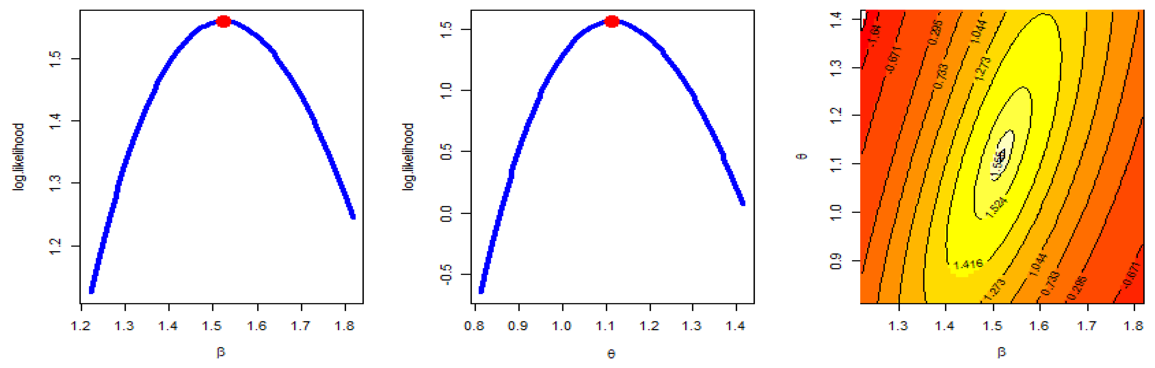
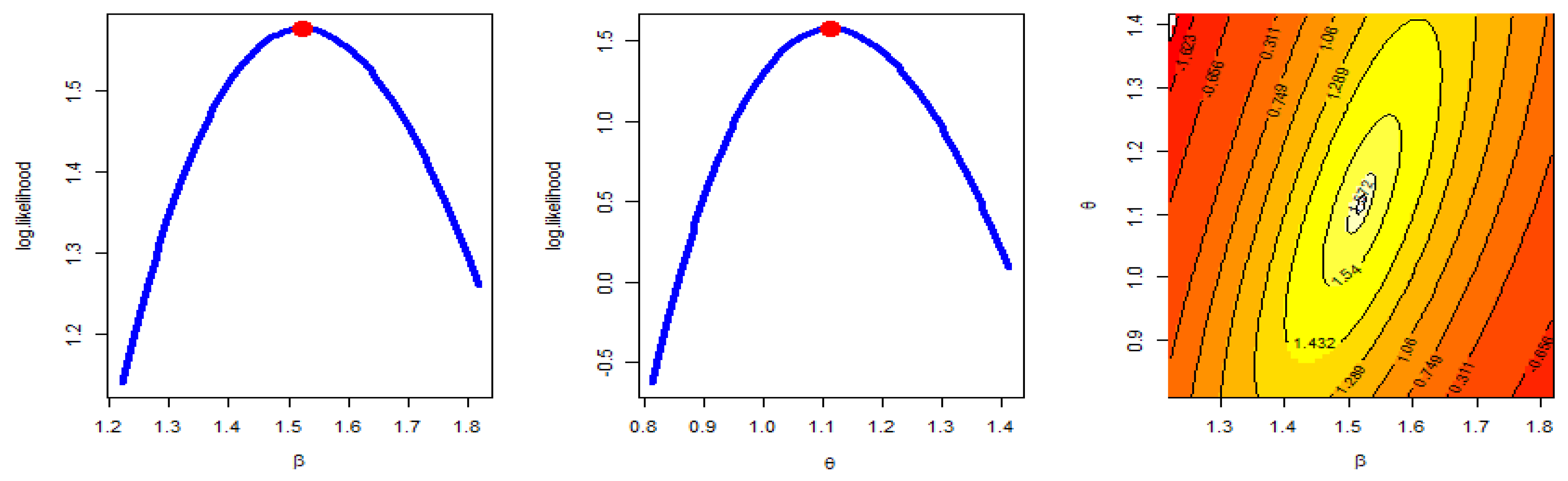
Figure 6, Figure 7 and Figure 8 were created to examine the maximum values of the estimators by profile likelihood as well as the existence and uniqueness of the log-likelihood function by contour plot with regard to different d and q options based on GPHCS-T2 samples with s = 25 and distinct p = 0.2, 0.5, and 0.8, respectively. Figure 9 clearly shows that the MCMC technique converged favorably and that the recommended size of the burn-in sample was adequate to completely nullify the impact of the recommended beginning values. Figure 9 demonstrates that the estimated estimates of and were roughly symmetrical for each sample when s = 25.
8. Conclusions and Discussion
This paper examines the reliability analysis of the unknown parameters, reliability, and hazard rate functions for the generalized type-II progressive hybrid censoring-based KMKu model. The “maxLik” package of the R programming language was used to compute the frequentist estimates with their asymptotic confidence intervals for the unknown parameters and any function of them. Since the likelihood function was produced in complex form, the posterior density function was obtained in nonlinear form. Consequently, the Bayesian estimates and the related HPD intervals were created using the Metropolis-Hastings technique and accounting for the squared error loss function. Numerous simulation experiments were run utilizing various total test unit choices, observed failure data, threshold times, and progressive censoring schemes in order to compare the behavior of the collected estimates. The outcomes demonstrated that the Bayes–MCMC strategy performed substantially better than the frequentist approach. Under generalized type-II progressive hybrid censoring, it was suggested to estimate the KMKu distribution’s parameters, reliability, and hazard functions using the Bayesian MCMC paradigm. We believe that the technique and results described here will be helpful to reliability practitioners and that they will be used to inform future censoring tactics. The 30 assessments of the tensile strength of polyester fibers are used to demonstrate how the recommended strategies may be applied in real-world circumstances. The most important results can be summarized in the following points:
- The key general finding is that the suggested values for and performed well.
- All estimations of R(t), and h(t) functioned satisfactorily as n (or s) grew.
- In most cases, the MSE, Bias, and WCI of all unknown parameters fell while their CPs grew as (T1, T2) increased.
- Due to the gamma information, the Bayes estimates of and behaved more predictably than the other estimates. Regarding credible HPD intervals, the same statement might be made.
- In most cases, the proposed estimates of and performed better when the parameter of binomial was increased.
- The MLE has a unique solution and a maximum value of log-likelihood.
Author Contributions
Conceptualization, R.A., E.M.A. and H.R.; methodology, R.A., E.M.A. and H.R.; writing—original draft preparation, R.A., E.M.A. and H.R.; writing—review and editing, R.A., E.M.A. and H.R. All the authors have the same contribution and agree to publish the manuscript in Symmetry Journal. All authors have read and agreed to the published version of the manuscript.
Funding
This research was funded by Princess Nourah bint Abdulrahman University Researchers Supporting Project number (PNURSP2023R50), Princess Nourah bint Abdulrahman University, Riyadh, Saudi Arabia.
Institutional Review Board Statement
Not applicable.
Informed Consent Statement
Not applicable.
Data Availability Statement
The data used to support the findings of this study are included within the article.
Acknowledgments
Princess Nourah bint Abdulrahman University Researchers Supporting Project number (PNURSP2023R50), Princess Nourah bint Abdulrahman University, Riyadh, Saudi Arabia.
Conflicts of Interest
The authors declare no conflict of interest.
References
- Balakrishnan, N.; Aggarwala, R. Progressive Censoring: Theory, Methods, and Applications; Springer Science & Business Media: Berlin, Germany, 2000. [Google Scholar]
- Balakrishnan, N. Progressive censoring methodology: An appraisal. TEST 2007, 16, 211–259. [Google Scholar] [CrossRef]
- Balakrishnan, N.; Cramer, E. The Art of Progressive Censoring; Springer: New York, NY, USA, 2014. [Google Scholar]
- Kundu, D.; Joarder, A. Analysis of Type-II progressively hybrid censored data. Comput. Stat. Data Anal. 2006, 50, 2509–2528. [Google Scholar] [CrossRef]
- Childs, A.; Chandrasekar, B.; Balakrishnan, N. Exact likelihood inference for an exponential parameter under progressive hybrid censoring schemes. In Statistical Models and Methods for Biomedical and Technical Systems; Vonta, F., Nikulin, M., Limnios, N., Huber-Carol, C., Eds.; Birkhäuser: Boston, MA, USA, 2008; pp. 319–330. [Google Scholar]
- Lee, K.; Sun, H.; Cho, Y. Exact likelihood inference of the exponential parameter under generalized Type II progressive hybrid censoring. J. Korean Stat. Soc. 2016, 45, 123–136. [Google Scholar] [CrossRef]
- Ateya, S.; Mohammed, H. Prediction under Burr-XII distribution based on generalized Type-II progressive hybrid censoring scheme. J. Egypt. Math. Soc. 2018, 26, 491–508. [Google Scholar]
- Seo, J.I. Objective Bayesian analysis for the Weibull distribution with partial information under the generalized Type-II progressive hybrid censoring scheme. Commun. Stat.-Simul. Comput. 2020, 51, 5157–5173. [Google Scholar] [CrossRef]
- Cho, S.; Lee, K. Exact likelihood inference for a competing risks model with generalized Type-II progressive hybrid censored exponential data. Symmetry 2021, 13, 887. [Google Scholar] [CrossRef]
- Nagy, M.; Bakr, M.E.; Alrasheedi, A.F. Analysis with applications of the generalized Type-II progressive hybrid censoring sample from Burr Type-XII model. Math. Probl. Eng. 2022, 2022, 1241303. [Google Scholar] [CrossRef]
- Alotaibi, N.; Elbatal, I.; Shrahili, M.; Al-Moisheer, A.S.; Elgarhy, M.; Almetwally, E.M. Statistical Inference for the Kavya–Manoharan Kumaraswamy Model under Ranked Set Sampling with Applications. Symmetry 2023, 15, 587. [Google Scholar] [CrossRef]
- Henningsen, A.; Toomet, O. maxlik: A package for maximum likelihood estimation in R. Comput Stat. 2011, 26, 443–458. [Google Scholar] [CrossRef]
- Plummer, M.; Best, N.; Cowles, K.; Vines, K. CODA: Convergence diagnosis and output analysis for MCMC. RNews 2006, 6, 7–11. [Google Scholar]
- Luo, C.; Shen, L.; Xu, A. Modelling and estimation of system reliability under dynamic operating environments and lifetime ordering constraints. Reliab. Eng. Syst. Saf. 2022, 218, 108136. [Google Scholar] [CrossRef]
- Shirong, Z.; Ancha, X.; Yincai, T.; Lijuan, S. Fast Bayesian Inference of Reparameterized Gamma Process with Random Effects. IEEE Trans. Reliab. 2023, 1–14. [Google Scholar] [CrossRef]
- Zhuang, L.; Xu, A.; Wang, X.-L. A prognostic driven predictive maintenance framework based on Bayesian deep learning. Reliab. Eng. Syst. Saf. 2023, 234, 109181. [Google Scholar] [CrossRef]
- Gelman, A.; Carlin, J.B.; Stern, H.S.; Rubin, D.B. Bayesian Data Analysis, 2nd ed.; Chapman and Hall/CRC: Boca Raton, FL, USA, 2004. [Google Scholar]
- Lynch, S.M. Introduction to Applied Bayesian Statistics and Estimation for Social Scientists; Springer: New York, NY, USA, 2007. [Google Scholar]
- Lawless, J.F. Statistical Models and Methods for Lifetime Data, 2nd ed.; John Wiley and Sons: Hoboken, NJ, USA, 1982. [Google Scholar]
- Greene, W.H. Econometric Analysis, 4th ed.; Prentice-Hall: New York, NY, USA, 2000. [Google Scholar]
- Chen, M.H.; Shao, Q.M. Monte Carlo estimation of Bayesian credible and HPD intervals. J. Comput. Graph. Stat. 1999, 8, 69–92. [Google Scholar]
- Ng, H.K.T.; Chan, P.S.; Balakrishnan, N. Optimal progressive censoring plans for the Weibull distribution. Technometrics 2004, 46, 470–481. [Google Scholar] [CrossRef]
- Pradhan, B.; Kundu, D. Inference and optimal censoring schemes for progressively censored Birnbaum–Saunders distribution. J. Stat. Plan. Inference 2013, 143, 1098–1108. [Google Scholar] [CrossRef]
- Alotaibi, R.; Mutairi, A.; Almetwally, E.M.; Park, C.; Rezk, H. Optimal Design for a Bivariate Step-Stress Accelerated Life Test with Alpha Power Exponential Distribution Based on Type-I Progressive Censored Samples. Symmetry 2022, 14, 830. [Google Scholar] [CrossRef]
- Dey, S.; Singh, S.; Tripathi, Y.M.; Asgharzadeh, A. Estimation and prediction for a progressively censored generalized inverted exponential distribution. Stat. Methodol. 2016, 32, 185–202. [Google Scholar]
Figure 1.
Generalized type-II progressive hybrid cases.

Figure 2.
Profile likelihood and contour plot s = 20 p = 0.2.

Figure 3.
Profile likelihood and contour plot s = 20 p = 0.5.

Figure 4.
Profile likelihood and contour plot s = 20 p = 0.8.

Figure 5.
Bayesian checks when s = 20.

Figure 6.
Profile likelihood and contour plot s = 25; p = 0.2.

Figure 7.
Profile likelihood and contour plot s = 25; p = 0.5.

Figure 8.
Profile likelihood and contour plot s = 25; p = 0.8.

Figure 9.
Bayesian checks when s = 25.


Table 1.
The notations of the GPHCS-T2.
| 1 | ||||
| 2 | s | 1 | 0 | |
| 3 |
Table 2.
Illustrations of numerous helpful censoring methods and best practices.
| Criterion | Method |
|---|---|
| Maximize trace | |
| Minimize trace | |
| Minimize det | |
| Minimize |
Table 3.
Bias, MSE, WCI, and CP for parameters and reliability measures: .
| MLE | Bayesian | |||||||||||
|---|---|---|---|---|---|---|---|---|---|---|---|---|
| n | r | s | Bias | MSE | WACI | CP | Optimality | Bias | MSE | WCCI | ||
| 30 | 0.3 | 20 | 0.3647 | 0.96096 | 3.5687 | 95.8% | 0.862132 | 0.0495 | 0.03658 | 0.9815 | ||
| 0.3083 | 0.30741 | 1.8074 | 95.3% | 0.050431 | 0.0652 | 0.0178 | 0.6268 | |||||
| R(0.6) | −1.0730 | 0.01021 | 3.5687 | 95.8% | 24.39956 | −1.0929 | 0.00159 | 0.9815 | ||||
| H(0.6) | 2.6011 | 2.15503 | 1.8074 | 95.3% | 0.397259 | 2.2794 | 0.15897 | 0.6268 | ||||
| R(0.85) | −1.3190 | 0.00311 | 3.5687 | 95.8% | −1.3269 | 0.00026 | 0.9815 | |||||
| H(0.85) | 9.8905 | 28.98923 | 1.8074 | 95.3% | 8.2579 | 1.30669 | 0.6268 | |||||
| 25 | 0.3133 | 0.68518 | 3.0049 | 96.0% | 0.603238 | 0.0348 | 0.01182 | 0.6606 | ||||
| 0.1931 | 0.20528 | 1.6075 | 95.7% | 0.028622 | 0.0196 | 0.00163 | 0.4069 | |||||
| R(0.6) | −1.0962 | 0.00644 | 3.0049 | 96.0% | 29.16632 | −1.1016 | 0.00050 | 0.6606 | ||||
| H(0.6) | 2.6177 | 1.64301 | 1.6075 | 95.7% | 0.637278 | 2.2792 | 0.05406 | 0.4069 | ||||
| R(0.85) | −1.3278 | 0.00190 | 3.0049 | 96.0% | −1.3295 | 0.00009 | 0.6606 | |||||
| H(0.85) | 9.6683 | 20.97684 | 1.6075 | 95.7% | 8.1852 | 0.42306 | 0.4069 | |||||
| 0.8 | 20 | 0.4478 | 1.11270 | 3.7458 | 95.6% | 0.897504 | 0.0686 | 0.04368 | 1.0098 | |||
| 0.2881 | 0.29977 | 1.8260 | 95.3% | 0.054545 | 0.0541 | 0.00853 | 0.6131 | |||||
| R(0.6) | −1.0925 | 0.00827 | 3.7458 | 95.6% | 23.77178 | −1.0994 | 0.00147 | 1.0098 | ||||
| H(0.6) | 2.7704 | 2.38574 | 1.8260 | 95.3% | 0.410967 | 2.3269 | 0.17886 | 0.6131 | ||||
| R(0.85) | −1.3285 | 0.00217 | 3.7458 | 95.6% | −1.3295 | 0.00025 | 1.0098 | |||||
| H(0.85) | 10.3764 | 33.31616 | 1.8260 | 95.3% | 8.3746 | 1.53529 | 0.6131 | |||||
| 25 | 0.3005 | 0.65995 | 2.9601 | 96.2% | 0.588428 | 0.0312 | 0.00897 | 0.6494 | ||||
| 0.1892 | 0.20103 | 1.5942 | 95.3% | 0.02822 | 0.0199 | 0.00162 | 0.4063 | |||||
| R(0.6) | −1.0954 | 0.00634 | 2.9601 | 96.2% | 28.83162 | −1.1009 | 0.00041 | 0.6494 | ||||
| H(0.6) | 2.5961 | 1.54340 | 1.5942 | 95.3% | 0.290327 | 2.2713 | 0.04112 | 0.4063 | ||||
| R(0.85) | −1.3273 | 0.00191 | 2.9601 | 96.2% | −1.3293 | 0.00008 | 0.6494 | |||||
| H(0.85) | 9.5939 | 20.02147 | 1.5942 | 95.3% | 8.1634 | 0.31889 | 0.4063 | |||||
| 50 | 0.3 | 35 | 0.2321 | 0.33855 | 2.0926 | 95.2% | 0.3524 | 0.0219 | 0.00682 | 0.2936 | ||
| 0.2206 | 0.16385 | 1.3310 | 94.8% | 0.0109 | 0.0389 | 0.00404 | 0.1817 | |||||
| R(0.6) | 0.0150 | 0.00491 | 0.2684 | 94.9% | 40.4391 | 0.0044 | 0.00056 | 0.0984 | ||||
| H(0.6) | 0.2660 | 0.86775 | 3.5013 | 95.4% | 0.4010 | 0.0230 | 0.03428 | 0.7479 | ||||
| R(0.85) | 0.0019 | 0.00151 | 0.1522 | 95.8% | 0.0005 | 0.00010 | 0.0418 | |||||
| H(0.85) | 1.2233 | 10.31472 | 11.6464 | 95.4% | 0.1173 | 0.24180 | 1.8061 | |||||
| 45 | 0.1009 | 0.17989 | 1.6157 | 95.3% | 0.2308 | 0.0127 | 0.00185 | 0.1390 | ||||
| 0.0688 | 0.07292 | 1.0241 | 95.5% | 0.0051 | 0.0080 | 0.00043 | 0.0697 | |||||
| R(0.6) | 0.0038 | 0.00306 | 0.2163 | 95.2% | 52.6779 | −0.0009 | 0.00013 | 0.0468 | ||||
| H(0.6) | 0.1237 | 0.55947 | 2.8931 | 95.4% | 0.3850 | 0.0228 | 0.00944 | 0.3526 | ||||
| R(0.85) | 0.0023 | 0.00099 | 0.1228 | 95.9% | −0.0008 | 0.00002 | 0.0202 | |||||
| H(0.85) | 0.5401 | 5.79962 | 9.2044 | 95.3% | 0.0729 | 0.06640 | 0.8489 | |||||
| 0.8 | 35 | 0.2292 | 0.33120 | 2.0704 | 95.7% | 0.3413 | 0.0302 | 0.00762 | 0.2866 | |||
| 0.1710 | 0.13353 | 1.2666 | 94.8% | 0.0103 | 0.0289 | 0.00277 | 0.1549 | |||||
| R(0.6) | 0.0043 | 0.00413 | 0.2516 | 94.5% | 40.8715 | 0.0003 | 0.00049 | 0.0905 | ||||
| H(0.6) | 0.2984 | 0.88222 | 3.4929 | 95.3% | 0.5510 | 0.0472 | 0.03668 | 0.6994 | ||||
| R(0.85) | −0.0013 | 0.00132 | 0.1424 | 95.8% | −0.0010 | 0.00009 | 0.0382 | |||||
| H(0.85) | 1.2328 | 10.27127 | 11.6023 | 95.7% | 0.1697 | 0.26968 | 1.7342 | |||||
| 45 | 0.1024 | 0.17088 | 1.6527 | 95.8% | 0.2313 | 0.0132 | 0.00183 | 0.1361 | ||||
| 0.0614 | 0.07091 | 1.0767 | 95.4% | 0.0052 | 0.0077 | 0.00047 | 0.0735 | |||||
| R(0.6) | 0.0020 | 0.00301 | 0.2196 | 95.0% | 52.8830 | −0.0011 | 0.00013 | 0.0450 | ||||
| H(0.6) | 0.1288 | 0.55691 | 2.9153 | 95.4% | 0.3953 | 0.0242 | 0.00934 | 0.3352 | ||||
| R(0.85) | 0.0018 | 0.00100 | 0.1240 | 95.6% | −0.0009 | 0.00002 | 0.0195 | |||||
| H(0.85) | 0.5493 | 5.70139 | 9.3735 | 95.9% | 0.0762 | 0.06541 | 0.8280 | |||||
| 100 | 0.3 | 70 | 0.1428 | 0.13884 | 1.3498 | 95.3% | 0.1469 | 0.0129 | 0.00257 | 0.1755 | ||
| 0.1269 | 0.06502 | 0.8674 | 95.3% | 0.0020 | 0.0189 | 0.00121 | 0.1107 | |||||
| R(0.6) | 0.0045 | 0.00218 | 0.1823 | 94.6% | 80.6294 | 0.0016 | 0.00021 | 0.0575 | ||||
| H(0.6) | 0.1901 | 0.40464 | 2.3807 | 95.0% | 0.6115 | 0.0162 | 0.01332 | 0.4378 | ||||
| R(0.85) | −0.0017 | 0.00065 | 0.0999 | 96.1% | −0.0001 | 0.00004 | 0.0249 | |||||
| H(0.85) | 0.7729 | 4.38212 | 7.6300 | 95.3% | 0.0702 | 0.09184 | 1.0646 | |||||
| 90 | 0.0668 | 0.07946 | 1.0740 | 95.7% | 0.1065 | 0.0062 | 0.00054 | 0.0852 | ||||
| 0.0497 | 0.03711 | 0.7299 | 95.5% | 0.0011 | 0.0045 | 0.00020 | 0.0495 | |||||
| R(0.6) | 0.0013 | 0.00162 | 0.1577 | 95.0% | 102.5854 | −0.0003 | 0.00005 | 0.0275 | ||||
| H(0.6) | 0.0898 | 0.25612 | 1.9533 | 94.7% | 0.8814 | 0.0107 | 0.00299 | 0.2093 | ||||
| R(0.85) | 0.0000 | 0.00050 | 0.0880 | 95.0% | −0.0004 | 0.00001 | 0.0120 | |||||
| H(0.85) | 0.3625 | 2.56087 | 6.1131 | 95.6% | 0.0351 | 0.01967 | 0.5192 | |||||
| 0.8 | 70 | 0.1309 | 0.13318 | 1.3361 | 95.4% | 0.1442 | 0.0146 | 0.00261 | 0.1649 | |||
| 0.1046 | 0.06010 | 0.8696 | 94.9% | 0.0020 | 0.0157 | 0.00107 | 0.1047 | |||||
| R(0.6) | 0.0020 | 0.00220 | 0.1838 | 94.7% | 80.5925 | 0.0005 | 0.00021 | 0.0568 | ||||
| H(0.6) | 0.1803 | 0.40288 | 2.3868 | 95.0% | 0.6090 | 0.0220 | 0.01361 | 0.4150 | ||||
| R(0.85) | −0.0018 | 0.00065 | 0.1001 | 95.9% | −0.0005 | 0.00004 | 0.0241 | |||||
| H(0.85) | 0.7125 | 4.25301 | 7.5901 | 95.2% | 0.0816 | 0.09367 | 1.0046 | |||||
| 90 | 0.0505 | 0.06859 | 1.0078 | 95.4% | 0.1039 | 0.0057 | 0.00047 | 0.0761 | ||||
| 0.0318 | 0.03404 | 0.7127 | 94.5% | 0.0011 | 0.0036 | 0.00019 | 0.0488 | |||||
| R(0.6) | 0.0004 | 0.00155 | 0.1544 | 95.2% | 103.7077 | −0.0004 | 0.00005 | 0.0271 | ||||
| H(0.6) | 0.0682 | 0.23049 | 1.8638 | 95.7% | 0.7099 | 0.0103 | 0.00266 | 0.1933 | ||||
| R(0.85) | 0.0003 | 0.00047 | 0.0853 | 95.4% | −0.0004 | 0.00001 | 0.0113 | |||||
| H(0.85) | 0.2743 | 2.23659 | 5.7659 | 95.4% | 0.0327 | 0.01719 | 0.4665 | |||||
Table 4.
Bias, MSE, WCI and CP for parameters and Reliability measures: .
| MLE | Bayesian | |||||||||||
|---|---|---|---|---|---|---|---|---|---|---|---|---|
| n | r | s | Bias | MSE | WACI | CP | Optimality | Bias | MSE | WCCI | ||
| 30 | 0.3 | 20 | 0.2883 | 0.66402 | 2.9892 | 95.1% | 0.5529 | 0.0373 | 0.0172 | 0.9061 | ||
| 0.0923 | 0.03017 | 0.5771 | 96.5% | 0.0045 | 0.0191 | 0.0010 | 0.2005 | |||||
| R(0.6) | −1.3142 | 0.00273 | 2.9892 | 95.1% | 156.4684 | −1.3223 | 0.0002 | 0.9061 | ||||
| H(0.6) | 4.4198 | 3.85075 | 0.5771 | 96.5% | 3.6685 | 3.8534 | 0.1199 | 0.2005 | ||||
| R(0.85) | −1.3780 | 0.00051 | 2.9892 | 95.1% | −1.3834 | 0.0000 | 0.9061 | |||||
| H(0.85) | 11.2462 | 28.57208 | 0.5771 | 96.5% | 9.6102 | 0.7761 | 0.2005 | |||||
| 25 | 0.2330 | 0.41596 | 2.3587 | 95.6% | 0.3694 | 0.0242 | 0.0044 | 0.6032 | ||||
| 0.0565 | 0.01912 | 0.4950 | 95.3% | 0.0024 | 0.0058 | 0.0001 | 0.1311 | |||||
| R(0.6) | −1.3222 | 0.00166 | 2.3587 | 95.6% | 187.5492 | −1.3244 | 0.0001 | 0.6032 | ||||
| H(0.6) | 4.3140 | 2.50974 | 0.4950 | 95.3% | 4.2533 | 3.8249 | 0.0314 | 0.1311 | ||||
| R(0.85) | −1.3812 | 0.00029 | 2.3587 | 95.6% | −1.3839 | 0.0000 | 0.6032 | |||||
| H(0.85) | 10.8980 | 18.07372 | 0.4950 | 95.3% | 9.5259 | 0.2003 | 0.1311 | |||||
| 0.8 | 20 | 0.3112 | 0.59476 | 2.7674 | 95.4% | 0.5183 | 0.0446 | 0.0176 | 0.9133 | |||
| 0.0862 | 0.02909 | 0.5773 | 95.3% | 0.0042 | 0.0168 | 0.0009 | 0.1972 | |||||
| R(0.6) | −1.3207 | 0.00218 | 2.7674 | 95.4% | 156.8018 | −1.3236 | 0.0002 | 0.9133 | ||||
| H(0.6) | 4.4902 | 3.51118 | 0.5773 | 95.3% | 1.9839 | 3.8741 | 0.1242 | 0.1972 | ||||
| R(0.85) | −1.3808 | 0.00036 | 2.7674 | 95.4% | −1.3838 | 0.0000 | 0.9133 | |||||
| H(0.85) | 11.4035 | 25.72157 | 0.5773 | 95.3% | 9.6601 | 0.7988 | 0.1972 | |||||
| 25 | 0.2760 | 0.46980 | 2.4606 | 94.4% | 0.3856 | 0.0304 | 0.0058 | 0.6125 | ||||
| 0.0560 | 0.01951 | 0.5019 | 95.5% | 0.0025 | 0.0054 | 0.0001 | 0.1304 | |||||
| R(0.6) | −1.3254 | 0.00173 | 2.4606 | 94.4% | 188.0939 | −1.3251 | 0.0001 | 0.6125 | ||||
| H(0.6) | 4.4269 | 2.85414 | 0.5019 | 95.5% | 10.4186 | 3.8416 | 0.0413 | 0.1304 | ||||
| R(0.85) | −1.3822 | 0.00027 | 2.4606 | 94.4% | −1.3842 | 0.0000 | 0.6125 | |||||
| H(0.85) | 11.1889 | 20.49050 | 0.5019 | 95.5% | 9.5678 | 0.2637 | 0.1304 | |||||
| 50 | 0.3 | 35 | 0.1928 | 0.26587 | 1.8755 | 95.3% | 0.2300 | 0.0209 | 0.00625 | 0.2453 | ||
| 0.0636 | 0.01464 | 0.4038 | 95.4% | 0.0010 | 0.0111 | 0.00034 | 0.0531 | |||||
| R(0.6) | 0.0022 | 0.00138 | 0.1454 | 96.0% | 266.3510 | 0.0003 | 0.00009 | 0.0379 | ||||
| H(0.6) | 0.4533 | 1.64429 | 4.7044 | 95.0% | 4.7886 | 0.0504 | 0.04467 | 0.6665 | ||||
| R(0.85) | 0.0017 | 0.00022 | 0.0583 | 95.2% | −0.0001 | 0.00001 | 0.0118 | |||||
| H(0.85) | 1.2631 | 11.59297 | 12.4008 | 95.4% | 0.1365 | 0.28360 | 1.6561 | |||||
| 45 | 0.1025 | 0.15357 | 1.4834 | 95.2% | 0.1528 | 0.0111 | 0.00136 | 0.1177 | ||||
| 0.0252 | 0.00856 | 0.3492 | 95.8% | 0.0005 | 0.0027 | 0.00005 | 0.0238 | |||||
| R(0.6) | 0.0010 | 0.00090 | 0.1177 | 95.9% | 332.8660 | −0.0007 | 0.00002 | 0.0179 | ||||
| H(0.6) | 0.2438 | 0.97587 | 3.7545 | 95.7% | 9.7083 | 0.0284 | 0.00981 | 0.3228 | ||||
| R(0.85) | 0.0015 | 0.00015 | 0.0473 | 95.2% | −0.0003 | 0.00000 | 0.0057 | |||||
| H(0.85) | 0.6769 | 6.72601 | 9.8189 | 95.4% | 0.0737 | 0.06177 | 0.7925 | |||||
| 0.8 | 35 | 0.2216 | 0.30042 | 1.9661 | 95.3% | 0.2360 | 0.0286 | 0.00733 | 0.2601 | |||
| 0.0591 | 0.01448 | 0.4111 | 95.5% | 0.0010 | 0.0097 | 0.00031 | 0.0514 | |||||
| R(0.6) | −0.0014 | 0.00128 | 0.1404 | 95.7% | 264.3238 | −0.0009 | 0.00009 | 0.0380 | ||||
| H(0.6) | 0.5296 | 1.84331 | 4.9029 | 95.3% | 6.8233 | 0.0715 | 0.05206 | 0.7134 | ||||
| R(0.85) | 0.0005 | 0.00020 | 0.0555 | 94.9% | −0.0004 | 0.00001 | 0.0117 | |||||
| H(0.85) | 1.4571 | 13.09846 | 12.9931 | 95.3% | 0.1886 | 0.33239 | 1.7468 | |||||
| 45 | 0.1251 | 0.17500 | 1.5656 | 94.3% | 0.1585 | 0.0147 | 0.00189 | 0.1420 | ||||
| 0.0244 | 0.00782 | 0.3334 | 95.3% | 0.0005 | 0.0023 | 0.00004 | 0.0228 | |||||
| R(0.6) | −0.0008 | 0.00097 | 0.1224 | 96.3% | 331.8112 | −0.0011 | 0.00003 | 0.0200 | ||||
| H(0.6) | 0.3053 | 1.12358 | 3.9811 | 94.4% | 3.4415 | 0.0380 | 0.01355 | 0.3838 | ||||
| R(0.85) | 0.0010 | 0.00015 | 0.0485 | 95.8% | −0.0004 | 0.00000 | 0.0064 | |||||
| H(0.85) | 0.8313 | 7.71142 | 10.3916 | 94.4% | 0.0977 | 0.08563 | 0.9557 | |||||
| 100 | 0.3 | 70 | 0.1020 | 0.10312 | 1.1941 | 96.0% | 0.0930 | 0.0071 | 0.00176 | 0.1407 | ||
| 0.0390 | 0.00642 | 0.2745 | 95.2% | 0.0002 | 0.0063 | 0.00013 | 0.0334 | |||||
| R(0.6) | 0.0012 | 0.00065 | 0.0997 | 94.9% | 526.4983 | 0.0006 | 0.00003 | 0.0220 | ||||
| H(0.6) | 0.2402 | 0.65129 | 3.0217 | 95.9% | 3.0162 | 0.0158 | 0.01276 | 0.3863 | ||||
| R(0.85) | 0.0007 | 0.00010 | 0.0386 | 95.3% | 0.0001 | 0.00002 | 0.0070 | |||||
| H(0.85) | 0.6667 | 4.49884 | 7.8970 | 96.1% | 0.0451 | 0.07991 | 0.9471 | |||||
| 90 | 0.0661 | 0.06870 | 0.9948 | 95.5% | 0.0688 | 0.0055 | 0.00046 | 0.0784 | ||||
| 0.0164 | 0.00369 | 0.2292 | 95.4% | 0.0001 | 0.0014 | 0.00002 | 0.0160 | |||||
| R(0.6) | −0.0005 | 0.00048 | 0.0858 | 95.7% | 654.6192 | −0.0003 | 0.00001 | 0.0117 | ||||
| H(0.6) | 0.1605 | 0.44507 | 2.5397 | 95.2% | 6.7361 | 0.0139 | 0.00338 | 0.2125 | ||||
| R(0.85) | 0.0003 | 0.00007 | 0.0332 | 95.6% | −0.0001 | 0.00001 | 0.0038 | |||||
| H(0.85) | 0.4370 | 3.01381 | 6.5894 | 95.3% | 0.0361 | 0.02109 | 0.5289 | |||||
| 0.8 | 70 | 0.1036 | 0.10480 | 1.2028 | 95.8% | 0.0929 | 0.0115 | 0.00204 | 0.1556 | |||
| 0.0320 | 0.00609 | 0.2791 | 95.3% | 0.0002 | 0.0050 | 0.00011 | 0.0339 | |||||
| R(0.6) | −0.0002 | 0.00064 | 0.0994 | 95.7% | 525.8864 | −0.0002 | 0.00004 | 0.0232 | ||||
| H(0.6) | 0.2484 | 0.66914 | 3.0567 | 95.8% | 4.7902 | 0.0283 | 0.01472 | 0.4259 | ||||
| R(0.85) | 0.0003 | 0.00009 | 0.0381 | 96.1% | −0.0002 | 0.00002 | 0.0073 | |||||
| H(0.85) | 0.6812 | 4.58927 | 7.9658 | 95.9% | 0.0754 | 0.09250 | 1.0493 | |||||
| 90 | 0.0652 | 0.07266 | 1.0258 | 95.7% | 0.0689 | 0.0060 | 0.00052 | 0.0794 | ||||
| 0.0161 | 0.00373 | 0.2310 | 95.1% | 0.0001 | 0.0013 | 0.00002 | 0.0161 | |||||
| R(0.6) | −0.0001 | 0.00052 | 0.0894 | 94.8% | 650.3684 | −0.0004 | 0.00001 | 0.0124 | ||||
| H(0.6) | 0.1583 | 0.47338 | 2.6260 | 95.6% | 6.4073 | 0.0153 | 0.00379 | 0.2188 | ||||
| R(0.85) | 0.0005 | 0.00008 | 0.0345 | 94.8% | −0.0002 | 0.00001 | 0.0040 | |||||
| H(0.85) | 0.4317 | 3.19473 | 6.8025 | 95.6% | 0.0396 | 0.02362 | 0.5400 | |||||
Table 5.
Bias, MSE, WCI and CP for parameters and Reliability measures: .
| MLE | Bayesian | |||||||||||
|---|---|---|---|---|---|---|---|---|---|---|---|---|
| n | r | s | Bias | MSE | WACI | CP | Optimality | Bias | MSE | WCCI | ||
| 30 | 0.3 | 20 | 0.0477 | 0.03572 | 0.7173 | 96.0% | 0.0822 | 0.0069 | 0.0009 | 0.2488 | ||
| 0.1693 | 0.10228 | 1.0642 | 95.4% | 0.0011 | 0.0454 | 0.0066 | 0.3352 | |||||
| R(0.6) | 0.0653 | 0.01134 | 0.7173 | 96.0% | 0.0822 | 0.0392 | 0.0014 | 0.2488 | ||||
| H(0.6) | 1.0736 | 0.26208 | 1.0642 | 95.4% | 0.0011 | 1.0039 | 0.0089 | 0.3352 | ||||
| R(0.85) | −0.1242 | 0.00977 | 0.7173 | 96.0% | −0.1418 | 0.0008 | 0.2488 | |||||
| H(0.85) | 3.1086 | 1.57995 | 1.0642 | 95.4% | 2.8625 | 0.0409 | 0.3352 | |||||
| 25 | 0.0420 | 0.02739 | 0.6279 | 95.8% | 0.0591 | 0.0051 | 0.0003 | 0.1640 | ||||
| 0.0938 | 0.05590 | 0.8511 | 94.9% | 0.0006 | 0.0139 | 0.0009 | 0.2075 | |||||
| R(0.6) | 0.0413 | 0.00854 | 0.6279 | 95.8% | 170.1243 | 0.0291 | 0.0003 | 0.1640 | ||||
| H(0.6) | 1.0797 | 0.21444 | 0.8511 | 94.9% | 5.0156 | 1.0038 | 0.0029 | 0.2075 | ||||
| R(0.85) | −0.1395 | 0.00729 | 0.6279 | 95.8% | −0.1478 | 0.0002 | 0.1640 | |||||
| H(0.85) | 3.0747 | 1.22571 | 0.8511 | 94.9% | 2.8470 | 0.0134 | 0.2075 | |||||
| 0.8 | 20 | 0.0747 | 0.04126 | 0.7408 | 96.2% | 0.0818 | 0.0116 | 0.0012 | 0.2625 | |||
| 0.1633 | 0.09437 | 1.0204 | 96.1% | 0.0011 | 0.0378 | 0.0051 | 0.3251 | |||||
| R(0.6) | 0.0443 | 0.01003 | 0.7408 | 96.2% | 131.1160 | 0.0330 | 0.0012 | 0.2625 | ||||
| H(0.6) | 1.1578 | 0.29506 | 1.0204 | 96.1% | 3.2292 | 1.0197 | 0.0110 | 0.3251 | ||||
| R(0.85) | −0.1436 | 0.00864 | 0.7408 | 96.2% | −0.1467 | 0.0007 | 0.2625 | |||||
| H(0.85) | 3.2918 | 1.79718 | 1.0204 | 96.1% | 2.8933 | 0.0527 | 0.3251 | |||||
| 25 | 0.0589 | 0.02782 | 0.6120 | 95.7% | 0.0592 | 0.0065 | 0.0003 | 0.1698 | ||||
| 0.0991 | 0.04971 | 0.7834 | 95.8% | 0.0006 | 0.0125 | 0.0006 | 0.2058 | |||||
| R(0.6) | 0.0296 | 0.00743 | 0.6120 | 95.7% | 159.3168 | 0.0275 | 0.0003 | 0.1698 | ||||
| H(0.6) | 1.1330 | 0.21505 | 0.7834 | 95.8% | 2.2242 | 1.0084 | 0.0034 | 0.2058 | ||||
| R(0.85) | −0.1517 | 0.00618 | 0.6120 | 95.7% | −0.1491 | 0.0002 | 0.1698 | |||||
| H(0.85) | 3.1924 | 1.23457 | 0.7834 | 95.8% | 2.8564 | 0.0157 | 0.2058 | |||||
| 50 | 0.3 | 35 | 0.0369 | 0.01839 | 0.5118 | 95.6% | 0.0387 | 0.0044 | 0.00032 | 0.0627 | ||
| 0.1055 | 0.04398 | 0.7108 | 95.9% | 0.0002 | 0.0229 | 0.00165 | 0.1006 | |||||
| R(0.6) | 0.0183 | 0.00581 | 0.2903 | 95.5% | 230.4277 | 0.0052 | 0.00044 | 0.0790 | ||||
| H(0.6) | 0.0795 | 0.14627 | 1.4672 | 95.2% | 2.9344 | 0.0102 | 0.00326 | 0.2111 | ||||
| R(0.85) | 0.0086 | 0.00523 | 0.2817 | 95.6% | 0.0021 | 0.00026 | 0.0627 | |||||
| H(0.85) | 0.2401 | 0.84128 | 3.4719 | 95.8% | 0.0328 | 0.01498 | 0.4164 | |||||
| 45 | 0.0292 | 0.01287 | 0.4300 | 95.8% | 0.0284 | 0.0031 | 0.00009 | 0.0311 | ||||
| 0.0523 | 0.02265 | 0.5534 | 95.8% | 0.0001 | 0.0065 | 0.00019 | 0.0406 | |||||
| R(0.6) | 0.0030 | 0.00414 | 0.2520 | 94.7% | 287.7103 | 0.0000 | 0.00010 | 0.0390 | ||||
| H(0.6) | 0.0702 | 0.10813 | 1.2599 | 95.7% | 3.0968 | 0.0088 | 0.00092 | 0.1034 | ||||
| R(0.85) | −0.0003 | 0.00374 | 0.2397 | 94.6% | −0.0008 | 0.00006 | 0.0317 | |||||
| H(0.85) | 0.1885 | 0.59457 | 2.9324 | 95.7% | 0.0220 | 0.00423 | 0.2099 | |||||
| 0.8 | 35 | 0.0451 | 0.01827 | 0.4997 | 95.6% | 0.0375 | 0.0065 | 0.00039 | 0.0608 | |||
| 0.0916 | 0.03438 | 0.6323 | 95.2% | 0.0002 | 0.0181 | 0.00104 | 0.0866 | |||||
| R(0.6) | 0.0071 | 0.00524 | 0.2826 | 95.7% | 223.9769 | 0.0018 | 0.00038 | 0.0752 | ||||
| H(0.6) | 0.1093 | 0.14684 | 1.4405 | 95.6% | 1.6721 | 0.0177 | 0.00378 | 0.2016 | ||||
| R(0.85) | −0.0004 | 0.00484 | 0.2727 | 95.5% | −0.0005 | 0.00024 | 0.0604 | |||||
| H(0.85) | 0.2965 | 0.83295 | 3.3853 | 95.6% | 0.0468 | 0.01780 | 0.4059 | |||||
| 45 | 0.0295 | 0.01341 | 0.4392 | 95.7% | 0.0280 | 0.0034 | 0.00010 | 0.0323 | ||||
| 0.0448 | 0.02086 | 0.5386 | 96.2% | 0.0001 | 0.0054 | 0.00016 | 0.0383 | |||||
| R(0.6) | 0.0003 | 0.00415 | 0.2525 | 93.7% | 288.9783 | −0.0006 | 0.00009 | 0.0395 | ||||
| H(0.6) | 0.0723 | 0.11132 | 1.2774 | 96.0% | 3.5188 | 0.0098 | 0.00097 | 0.1069 | ||||
| R(0.85) | −0.0018 | 0.00383 | 0.2426 | 94.8% | −0.0012 | 0.00006 | 0.0328 | |||||
| H(0.85) | 0.1896 | 0.61493 | 2.9842 | 95.8% | 0.0236 | 0.00451 | 0.2164 | |||||
| 100 | 0.3 | 70 | 0.0267 | 0.00855 | 0.3473 | 95.7% | 0.0171 | 0.0024 | 0.00012 | 0.0376 | ||
| 0.0690 | 0.01783 | 0.4484 | 95.0% | 0.0000 | 0.0117 | 0.00043 | 0.0568 | |||||
| R(0.6) | 0.0090 | 0.00284 | 0.2061 | 95.8% | 442.4535 | 0.0026 | 0.00016 | 0.0489 | ||||
| H(0.6) | 0.0645 | 0.07290 | 1.0283 | 95.1% | 2.9947 | 0.0057 | 0.00125 | 0.1240 | ||||
| R(0.85) | 0.0020 | 0.00263 | 0.2008 | 95.7% | 0.0010 | 0.00010 | 0.0387 | |||||
| H(0.85) | 0.1797 | 0.40180 | 2.3841 | 95.5% | 0.0177 | 0.00568 | 0.2530 | |||||
| 90 | 0.0129 | 0.00536 | 0.2827 | 94.7% | 0.0128 | 0.0013 | 0.00003 | 0.0181 | ||||
| 0.0256 | 0.00907 | 0.3597 | 95.0% | 0.0000 | 0.0029 | 0.00006 | 0.0233 | |||||
| R(0.6) | 0.0024 | 0.00205 | 0.1771 | 95.8% | 572.9885 | 0.0000 | 0.00003 | 0.0222 | ||||
| H(0.6) | 0.0310 | 0.04803 | 0.8508 | 94.7% | 2.3973 | 0.0038 | 0.00031 | 0.0595 | ||||
| R(0.85) | 0.0007 | 0.00187 | 0.1696 | 94.9% | −0.0003 | 0.00002 | 0.0179 | |||||
| H(0.85) | 0.0838 | 0.25437 | 1.9506 | 94.9% | 0.0096 | 0.00137 | 0.1225 | |||||
| 0.8 | 70 | 0.0274 | 0.00795 | 0.3328 | 95.3% | 0.0168 | 0.0034 | 0.00013 | 0.0392 | |||
| 0.0565 | 0.01500 | 0.4261 | 95.1% | 0.0000 | 0.0098 | 0.00034 | 0.0558 | |||||
| R(0.6) | 0.0035 | 0.00280 | 0.2070 | 94.8% | 441.2820 | 0.0011 | 0.00015 | 0.0484 | ||||
| H(0.6) | 0.0693 | 0.06869 | 0.9913 | 94.9% | 3.2956 | 0.0092 | 0.00133 | 0.1304 | ||||
| R(0.85) | −0.0016 | 0.00254 | 0.1976 | 95.5% | −0.0002 | 0.00010 | 0.0390 | |||||
| H(0.85) | 0.1834 | 0.37293 | 2.2845 | 94.9% | 0.0243 | 0.00610 | 0.2614 | |||||
| 90 | 0.0109 | 0.00515 | 0.2782 | 95.1% | 0.0127 | 0.0013 | 0.00003 | 0.0183 | ||||
| 0.0212 | 0.00904 | 0.3635 | 95.5% | 0.0000 | 0.0026 | 0.00005 | 0.0248 | |||||
| R(0.6) | 0.0022 | 0.00212 | 0.1802 | 95.2% | 577.1218 | 0.0000 | 0.00003 | 0.0236 | ||||
| H(0.6) | 0.0253 | 0.04644 | 0.8393 | 94.9% | 2.5652 | 0.0037 | 0.00028 | 0.0612 | ||||
| R(0.85) | 0.0011 | 0.00191 | 0.1712 | 94.9% | −0.0004 | 0.00002 | 0.0190 | |||||
| H(0.85) | 0.0693 | 0.24508 | 1.9224 | 94.9% | 0.0092 | 0.00125 | 0.1231 | |||||
Table 6.
MLE and Bayesian estimation.
| MLE | Bayesian | |||||||||
|---|---|---|---|---|---|---|---|---|---|---|
| Estimates | SE | R(0.6) | R(0.85) | Estimates | SE | R(0.6) | R(0.85) | |||
| s | p | H(0.6) | H(0.85) | H(0.6) | H(0.85) | |||||
| 20 | 0.2 | 0.8884 | 0.5264 | 0.3253 | 0.1189 | 0.9884 | 0.3296 | 0.3047 | 0.1017 | |
| 1.0033 | 0.2514 | 2.7480 | 6.4884 | 1.0556 | 0.2365 | 2.9811 | 7.1010 | |||
| 0.5 | 1.5376 | 0.5760 | 0.2111 | 0.0436 | 1.3577 | 0.3243 | 0.2505 | 0.0608 | ||
| 1.2293 | 0.2692 | 4.1919 | 10.4235 | 1.2399 | 0.1761 | 3.7759 | 9.3192 | |||
| 0.8 | 1.5404 | 0.5751 | 0.2091 | 0.0431 | 1.6921 | 0.3877 | 0.1800 | 0.0324 | ||
| 1.2231 | 0.2677 | 4.2022 | 10.4439 | 1.2090 | 0.1681 | 4.5521 | 11.3874 | |||
| 25 | 0.2 | 1.4928 | 0.4925 | 0.1858 | 0.0392 | 1.5520 | 0.3081 | 0.1795 | 0.0360 | |
| 1.0776 | 0.2203 | 4.1819 | 10.2139 | 1.0966 | 0.1464 | 4.3074 | 10.5745 | |||
| 0.5 | 1.5231 | 0.5001 | 0.1884 | 0.0389 | 1.5572 | 0.3157 | 0.1811 | 0.0362 | ||
| 1.1143 | 0.2294 | 4.2299 | 10.3859 | 1.1085 | 0.1507 | 4.3121 | 10.6013 | |||
| 0.8 | 1.5221 | 0.4996 | 0.1883 | 0.0389 | 1.4511 | 0.3053 | 0.2044 | 0.0451 | ||
| 1.1129 | 0.2293 | 4.2285 | 10.3804 | 1.1252 | 0.1523 | 4.0571 | 9.9345 | |||
Disclaimer/Publisher’s Note: The statements, opinions and data contained in all publications are solely those of the individual author(s) and contributor(s) and not of MDPI and/or the editor(s). MDPI and/or the editor(s) disclaim responsibility for any injury to people or property resulting from any ideas, methods, instructions or products referred to in the content. |
© 2023 by the authors. Licensee MDPI, Basel, Switzerland. This article is an open access article distributed under the terms and conditions of the Creative Commons Attribution (CC BY) license (https://creativecommons.org/licenses/by/4.0/).
Share and Cite
MDPI and ACS Style
Alotaibi, R.; Almetwally, E.M.; Rezk, H. Reliability Analysis of Kavya Manoharan Kumaraswamy Distribution under Generalized Progressive Hybrid Data. Symmetry 2023, 15, 1671. https://0-doi-org.brum.beds.ac.uk/10.3390/sym15091671
AMA Style
Alotaibi R, Almetwally EM, Rezk H. Reliability Analysis of Kavya Manoharan Kumaraswamy Distribution under Generalized Progressive Hybrid Data. Symmetry. 2023; 15(9):1671. https://0-doi-org.brum.beds.ac.uk/10.3390/sym15091671
Chicago/Turabian StyleAlotaibi, Refah, Ehab M. Almetwally, and Hoda Rezk. 2023. "Reliability Analysis of Kavya Manoharan Kumaraswamy Distribution under Generalized Progressive Hybrid Data" Symmetry 15, no. 9: 1671. https://0-doi-org.brum.beds.ac.uk/10.3390/sym15091671
Note that from the first issue of 2016, this journal uses article numbers instead of page numbers. See further details here.