Article

Methodology for Solving Engineering Problems of Burgers–Huxley Coupled with Symmetric Boundary Conditions by Means of the Network Simulation Method

by
Juan Francisco Sánchez-Pérez
1,
Fulgencio Marín-García
2,*,
Enrique Castro
1,
Gonzalo García-Ros
3,
Manuel Conesa
1 and
Joaquín Solano-Ramírez
4
1
Department of Applied Physics and Naval Technology, Universidad Politécnica de Cartagena (UPCT), 30202 Cartagena, Spain
2
Department of Automation Engineering, Electrical Engineering and Electronic Technology, Universidad Politécnica de Cartagena (UPCT), 30202 Cartagena, Spain
3
Department of Mining and Civil Engineering, Universidad Politécnica de Cartagena (UPCT), 30202 Cartagena, Spain
4
Department of Thermal Engineering and Fluids, Universidad Politécnica de Cartagena (UPCT), 30202 Cartagena, Spain
*
Author to whom correspondence should be addressed.
Submission received: 25 July 2023 / Revised: 27 August 2023 / Accepted: 7 September 2023 / Published: 11 September 2023
(This article belongs to the Special Issue Differential Equations and Applied Mathematics)

Abstract

:
The Burgers–Huxley equation is a partial differential equation which is based on the Burgers equation, involving diffusion, accumulation, drag, and species generation or sink phenomena. This equation is commonly used in fluid mechanics, air pollutant emissions, chloride diffusion in concrete, non-linear acoustics, and other areas. A general methodology is proposed in this work to solve the mentioned equation or coupled systems formed by it using the network simulation method. Additionally, the implementation of the most common possible boundary conditions in different engineering problems is indicated, including the Neumann condition that enables symmetry to be applied to the problem, reducing computation times. The method consists mainly of establishing an analogy between the variables of the differential equations and the electrical voltage at a central node. The methodology is also explained in detail, facilitating its implementation to similar engineering problems, since the equivalence, for example, between the different types of spatial and time derivatives and its correspondence with the electrical device is detailed. As an example, several cases of both the equation and a coupled system are solved by varying the boundary conditions on one side and applying symmetry on the other.

1. Introduction

The Burgers–Huxley equation is a partial differential equation [1,2], based on the Burgers equation, which involves accumulation, diffusion, drag, and species generation or sink phenomena. This or similar equations [3,4,5,6], together with its approximate solutions, are common in many areas of science and engineering, such as fluid mechanics [7,8], heat transmission [9,10,11,12,13,14], air pollutant emissions [15,16,17], chloride diffusion in concrete [18,19,20,21,22,23,24], nonlinear acoustics [25,26], optical fibres [27,28,29,30,31,32], and other areas. For example, pollutant emission problems include phenomena of accumulation, drag, diffusion, and in some cases chemical reactions [33]. Likewise, the diffusion problems of chlorides in reinforced concrete include all these phenomena of accumulation, drag, and diffusion [18], so all these problems could be solved through a common methodology with minor variations.
Thus, proposing a methodology for solving this equation or coupled systems of equations formed by variants of it is important due to its widespread applicability, since, as indicated above, numerous problems in engineering or science are variants of it.
On the other hand, in order to try to provide a general methodology for solving this type of problem, it is not enough to merely indicate how the equation should be solved, but also how the most common boundary conditions should be implemented. Therefore, the way to implement boundary conditions, such as Neumann’s or Dirichlet’s, among others, is indicated.
One of the most important of these conditions is the symmetry condition, whose importance lies in the fact that in 1D, 2D, and 3D problems it enables the study medium to be reduced and, thus, shortens the simulation time. Its applicability stands out in numerous engineering problems where there is symmetry, such as in cylindrical or square columns, either for the study of heat transmission, chloride diffusion, etc., or its application to different types of storage tanks where several phenomena can be studied [34,35,36].
Thus, as indicated above, having a methodology for solving this equation, or a system of coupled equations formed by variants of it, can prove extremely useful, as it facilitates the resolution of different problems in science and engineering.
In the present paper, a resolution methodology is proposed using the Network Simulation Method, NSM, which will indicate how this equation, or its variants, should be solved and how the boundary conditions should be implemented. This method has been chosen because NSM has been used efficiently in numerous science and engineering problems, including heat transfer [37,38,39], chloride diffusion [40], soil consolidation [41], etc.
In this way, the main purpose of the present article is to propose a resolution methodology, applying NSM, which is valid for solving symmetric or asymmetric problems that include the different variants of the Burgers–Huxley equation, or coupled systems of equations of it, with the most common boundary conditions for this type of problem. Thus, the novelty of this paper lies in it presenting a clear and concise methodology that allows science and engineering problems which include a partial differential equation or coupled systems of the same that imply phenomena of diffusion, drag, accumulation, and generation or decay of species to be easily solved, with variations of the most common boundary conditions, as well as different initial conditions.
The paper is structured as follows: Section 1 contains the introduction; then, the fundamentals of the network simulation method are explained in Section 2. The following section details the different mathematical models related to the Burgers–Huxley equation so that their network models are built in Section 4 with what is specified in Section 2. The results of different case studies are shown in Section 5. Finally, the conclusions of the paper are presented in Section 6.

2. Network Simulation Method

The network simulation method is used to solve complex systems with multiple variables, coupled and with non-linear relationships in science and engineering. The technique is based on building an electrical circuit, whose nodes are interconnected, representing the study problem, where the variables of interest (temperature, velocity, etc.) are the voltage at the central node [42].
The network simulation method has been used in numerous problems including the simulation of biological, social, and economic systems, among others. In engineering, the network method has been efficiently applied to electrochemical reactions [39], heat transport and coupled flow problems [13,38], membranes, soil mechanics [41], and oxidation problems [42], among others. One of the main characteristics of the method is that it requires thorough knowledge of the problem to be studied when constructing the network circuit. Thus, the geometry of the problem must be taken into account (Cartesian, spherical, cylindrical, 1D, 2D, and 3D coordinates, etc.), the precision of the necessary meshing, the precision parameters of the circuit resolution software, etc., in order to avoid obtaining erroneous results or the system not converging.
Thus, the main advantages of the method are as follows:
  • It allows us to work with ideal electrical components.
  • There is an almost intuitive relationship between the addends of the equation and the electrical components.
  • It has extensive component libraries available.
  • It provides very precise solutions thanks to the fact that the software includes trapezoidal integration and Gear’s fixed time methods, reducing the local truncation error and allowing model convergence.
  • It requires a relatively short execution time.
  • It only requires a limited number of software programming rules.
  • The software parameters, such as RELTOL and VNTOL, allow us to improve the precision of the solutions and the convergence of the system.
The main disadvantage of the method is that in very complex systems a very fine mesh is required, as occurs with any other similar simulation methodology, in order to obtain precise solutions so that the system can converge.
If we compare the method with other similar software, the methodology has turned out to be more precise [43], or the same results have been obtained as with commercial software [42], the disadvantage being that the latter only allow the problems for which they are programmed to be solved. Finally, the same results have been obtained as those obtained experimentally [42]. Thus, the main advantage of the methodology compared to other software is that it enables us to solve the study problem with precise results using a few straightforward programming rules.
Although the models will be described in detail in the appropriate section, a simple synthesis of the procedure is as follows:
  • First, the equivalence between the study variable and the voltage at the network nodes is established.
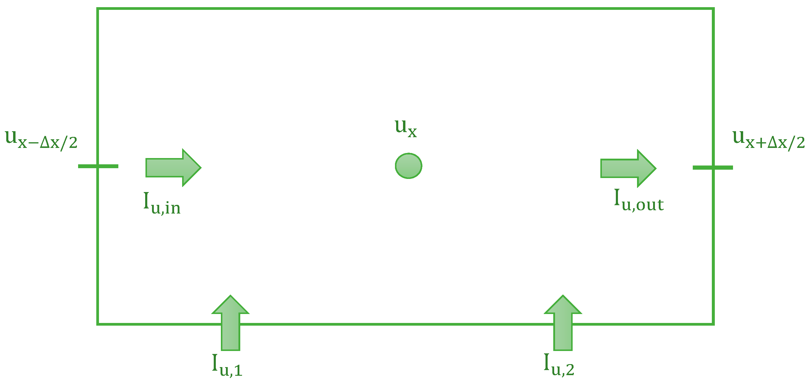
  • Secondly, the space is discretised in volume elements.
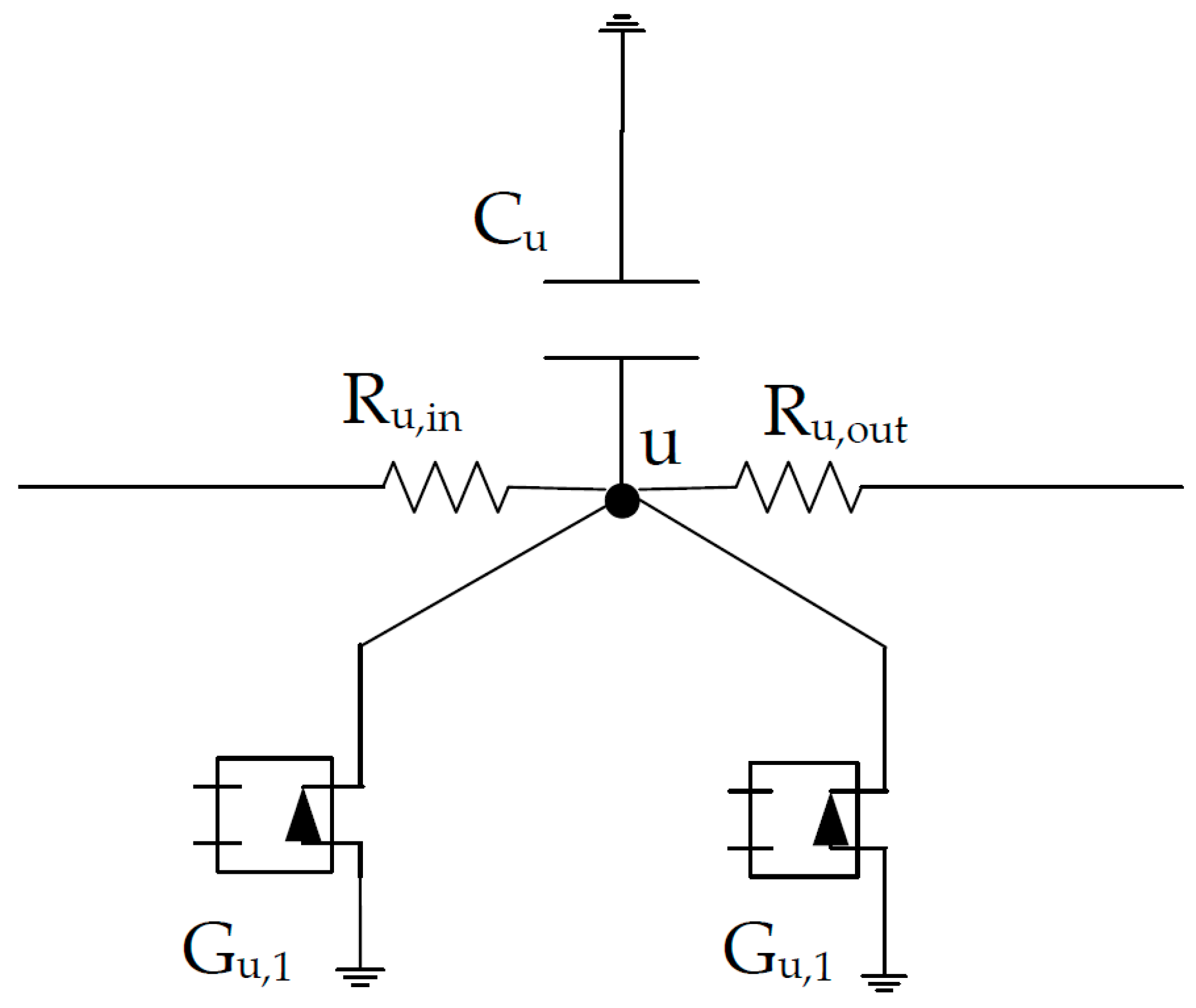
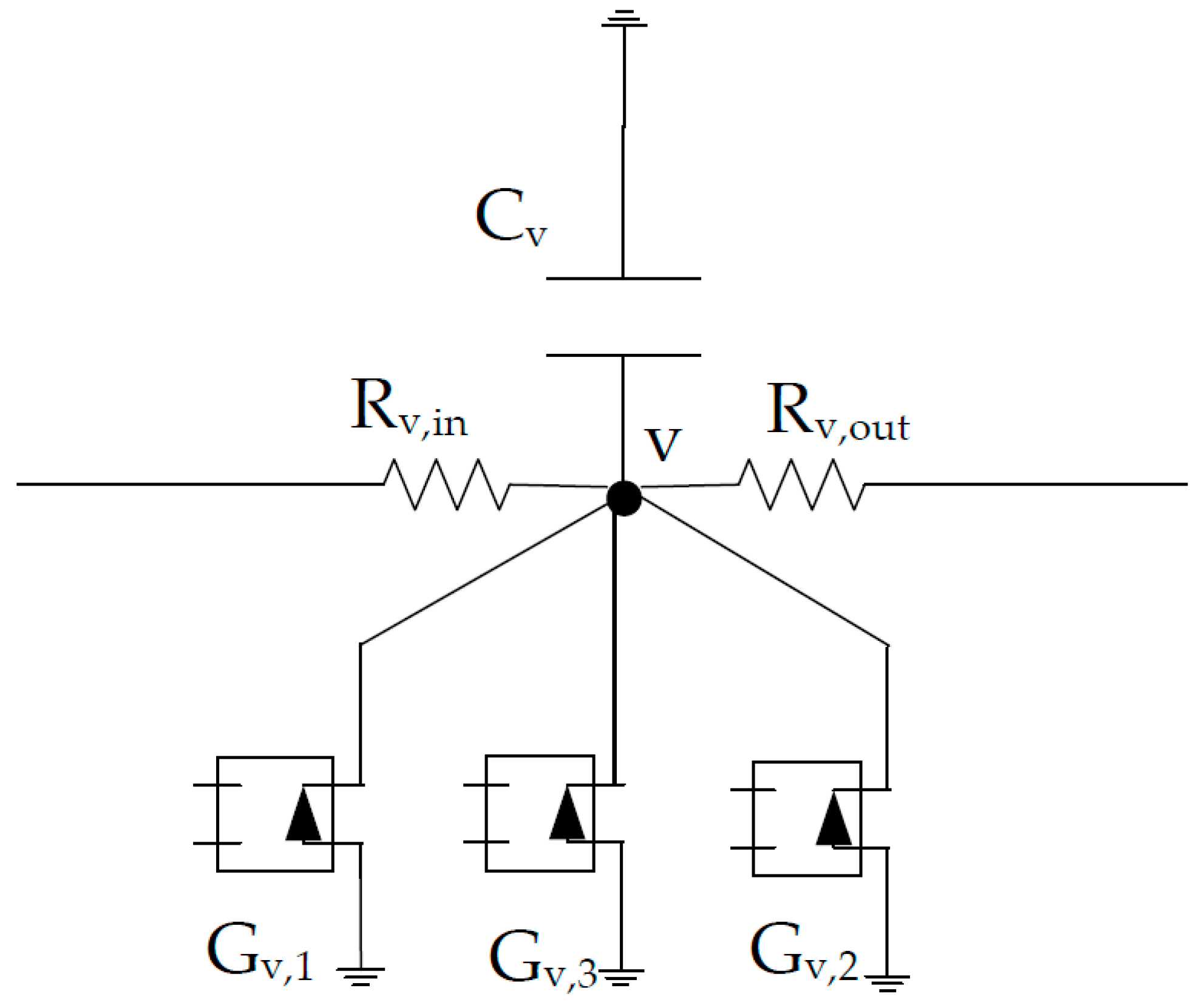
  • Finally, the addends of the previous equations are implemented as electrical elements, such as resistors, voltage sources, etc.
Focusing on the last point, we now propose a series of equivalences between the mathematical operation and the corresponding electrical device, which, although other devices could be used, can serve as an application guide. Once the equivalent circuit has been created, it is solved with circuit simulation software, such as NgSpice. The manual for that software provides detailed explanations as to how each element of the circuit should be implemented, as well as functions (sine, cosine, logarithm, etc.), conditionals, etc. [44].

2.1. The Concept of the Time Derivative

The rate at which a variable changes with respect to time is referred to as the time derivative in NgSpice. It is very important to understand this time derivative to analyse the behaviour of circuits over time using the software program NgSpice v36 [44]. Variables that change dynamically over time, such as voltages and currents, are frequently encountered when simulating circuits using NgSpice. The correct circuit components and functions in NgSpice simulations to account for the time derivative must be employed, for example, by using time-varying voltage sources, such as pulse or sinusoidal sources, and studying the behaviour of currents or voltages at various locations in the circuit. Overall, the time derivative concept in NgSpice enables us to study how circuit variables change over time and aids comprehension of the transient response of the circuit under different circumstances.

2.2. The Concept of the First Spatial Derivative

The rate at which a physical quantity changes in relation to spatial coordinates is referred to as the first spatial derivative in NgSpice. The first spatial derivative tells us how the quantity modifies as we move along the spatial coordinate. The user typically defines the required elements and specifies the appropriate boundary conditions or sources that affect the spatial variations in order to include the first spatial derivative in NgSpice simulations. Once the circuit equations and the specified spatial dependencies have been determined, NgSpice will calculate the first spatial derivative [44]. The way in which different quantities in a circuit or system change and behave spatially can be understood by looking at their first spatial derivative. This knowledge is essential for researching processes affected by spatial variations, such as heat transfer and signal propagation.

2.3. The Concept of the Second Spatial Derivative

The second spatial derivative of a physical quantity with respect to space or distance is the rate at which the first spatial derivative of that quantity changes. This derivative is important for understanding the curvature or change in a physical quantity within a circuit layout in the software program, which is used to simulate electronic circuits. It sheds light on the spatial gradients and variations of that quantity. The rate of change in the current gradient along the circuit path can be determined using NgSpice by calculating the second spatial derivative of the current with respect to the spatial coordinate. These insights are helpful in locating potential signal distortion, voltage drops, or circuit design inefficiencies. In summary, the second spatial derivative in NgSpice measures the rate at which a physical quantity, like current, changes its gradient with respect to a spatial coordinate inside an electronic circuit.
When studying mechanical problems, the fundamental variable is the position, usually defined by the letter “x”, just as the fundamental variable in circuit theory is the electric charge, defined as “q”. The next step is to establish a relationship between the variables of the mechanical problems and circuit theory. Starting with the capacitor, it is established that the constitutive equation of the capacitor is as follows:
i t = C · d u C ( t ) d t
by clearing the voltage across the capacitor, the following can be seen:
u C t = 1 C · t i t · d t
Since the variation of the charge with time is the current itself, as follows:
i t = d q ( t ) / d t
Then
d q t = i t · d t
and
d q t = i t · d t
Then
q t = i t · d t
This leads us to the conclusion that the voltage across the capacitor gives us the position since:
u C t = q ( t )
So
q t = x t
By studying the resistor, we obtain the velocity, as follows:
v t = d x ( t ) d t
and the variation of the charge with time is the current, as follows:
u R t = R · i t = R · d q ( t ) d t
Thus, the voltage in the resistor can be defined as the variable equivalent to the velocity.
For the acceleration, we study the coil or inductance. Acceleration is the variation of velocity with respect to time, as follows:
a t = d v ( t ) d t = d 2 x ( t ) d t 2
Therefore, following the reasoning for the velocity, we must derive twice the load, or the current only once, which is the same, as follows:
d 2 q ( t ) d t 2 = d i ( t ) d t
And the voltage across the coil is defined as follows:
u L t = L · d i ( t ) d t
Thus, the voltage in the coil is the acceleration multiplied by L.
In the above equations, the following terms appear: “C”, which is the capacitance of the capacitor whose unit is the farad (F), “R”, which is the value of the resistance in ohms (Ω), and “L”, which is the self-induction coefficient of the coil, whose unit of measurement is the Henry (H). These three terms must be established in accordance with the problem to be analysed for the multiplying coefficients that carry in each case, i.e., the position, velocity, and acceleration.

2.4. Remaining Addends

The incorporation of other terms of the equation which are not derivatives can be carried out, in most cases, by adding current sources. In an electrical circuit, a current source provides a current to a certain node which, due to Kirchhoff’s law of current, is added to the rest of the currents supplied by other branches or elements. Therefore, the incorporation of a current source to a node of the network is equivalent to the addition of a term in the equation. By defining the value of the current source as being equal to the term equation, it is incorporated into the volume element of the network model.

2.5. Boundary Conditions

The boundary conditions of the problem are incorporated into the network model by implementing them into the volume elements of the boundary. This implementation depends on the type of conditions and always implies the modification of the volume element of the network model in the boundary by changing one of its electric components or adding a new one.

2.5.1. Dirichlet’s Boundary Condition

A Dirichlet boundary condition means that the value of the variable in the boundary is fixed or depends on a function, which can be time- and/or spatially dependant. It can be expressed mathematically as follows:
u s = f ( s , t )
where s indicates the points of the boundary and t indicates the time.
As the value of u in a node of the network model can be fixed by a voltage source, a Dirichlet boundary condition is implemented by the connection of a voltage source to the node corresponding to the boundary. The value of the voltage source is determined by the function f(s, t), so the voltage source can have a constant value, if u is constant, or it can be a time-dependent source if u changes with time.
However, as there are no volume elements outside the boundary, the resistor of the boundary element that is not connected with any other volume element must be eliminated.

2.5.2. Neumann’s Boundary Condition

A Neumann’s boundary condition means that the value of the spatial derivative is fixed or depends on a function. It can be expressed mathematically as follows:
u x s = f ( s , t )
As the spatial derivative is the equivalent of the current in the NSM, a Neumann’s boundary condition can be implemented in the resistor that is not connected with another volume element in the volume element of the boundary. In the case of u x s = 0 , it means that there is no current going outside the system, so it can be implemented using a resistor with a very high resistance (theoretically infinite). In all other cases, the resistor is substituted by a current source with a value determined by f(s, t), or f(s), if it is time-independent.

2.5.3. Symmetry Boundary Condition

The symmetry condition is implemented as a Neumann condition, since introducing a resistance of theoretically infinite value does not allow the current, and, therefore, the flow of the variable under study, to leave the system. In this way, the spatial representation of the variable shows us half of its behaviour in the medium, with the other part’s behaviour being symmetrical to the half represented. This condition is particularly important since it saves computing time and reduces study space.

2.5.4. Displacement-Type Boundary Conditions

Displacement-type boundary conditions specify the behaviour of the displacement field of a physical system at the boundaries. They describe how the system responds to external forces or constraints applied at its boundaries. These conditions are expressed in terms of displacements or deformation components, as follows:
u ( s ,   t ) = f ( s , t )
where u(s, t) represents the displacement as a function of position s and time t, and f(s, t) is the function describing the displacement boundary condition at the boundary of the domain. In most cases the displacement condition applies to the extremes and usually has constant values over time, u ( 0 ,   t ) = u ( L ,   t ) = u 0 , or a value of zero, u ( 0 ,   t ) = u ( L ,   t ) = 0 . These displacement conditions are applied in NSM through a controlled voltage source connected to the edge node [45,46,47,48].

2.5.5. General Boundary Conditions

It is possible to have more general boundary conditions. In such cases, it is necessary to study the problem and determine the best way to implement the boundary conditions using the equivalence between the variables of the problem and the voltage and current of the network model. As the boundary conditions are imposed over the variable or its spatial derivatives at the boundary, it requires the use of current or voltage sources, or a mix of them. The addition of more electrical elements is sometimes necessary to obtain the values that must be introduced in the current or voltage source, for instance, in the simulation of longitudinal or transversal vibrations of a rod with an attached mass at one of its ends. In this case, it is necessary to add two auxiliary circuits to calculate the value of the boundary current source because it depends on the second temporal derivative of the position of the attached mass [49].

2.6. Initial Conditions

The initial conditions are implemented in the capacitor value of the first time derivative. Thus, as will be shown later, a different initial value can be assigned to each volume element of the spatial discretisation. Therefore, different initial conditions can be implemented, such as the Riemann problem, where the problem presents constant initial values that have a single discontinuity, as follows [50]:
u ( x ,   0 ) = u L                   x < a u R                   x a
where uL and uR are the initial values and a is the position where the discontinuity occurs. On the other hand, this methodology also allows the implementation of other types of initial variables, such as a distribution through a trigonometric or logarithmic function. Finally, when the network model does not include a capacitor, the initial conditions are implemented with the NgSpice “.ic” command [44].

2.7. Auxiliary Circuits

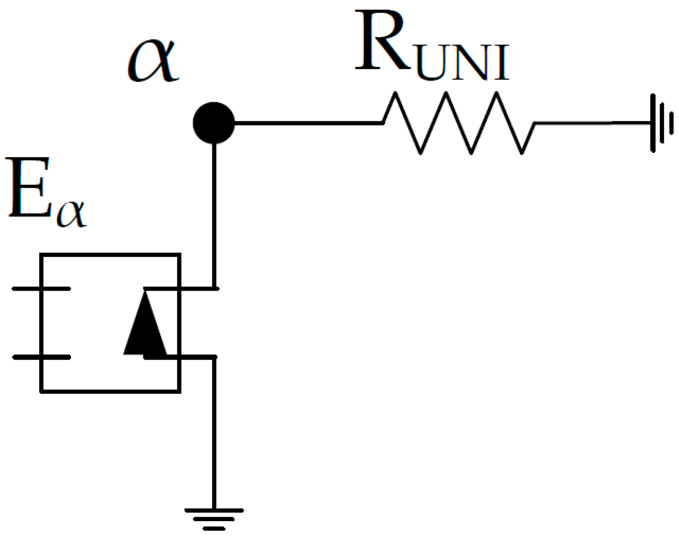
2.7.1. Time Generators

In some engineering problems it is necessary to operate with a variable, as will be seen in Section 5. In these cases, a time generator is implemented by means of an auxiliary circuit consisting of a unit value resistor and a voltage source that includes the “Piecewise Linear Function”, where it is indicated how the voltage should follow the time.

2.7.2. Other Equations

When we encounter equations, such as T = ax + b or T = ax2 + bsin(x), they are implemented as a circuit composed of a unity value resistor and non-linear dependent voltage sources, which is where the equation is implemented.

3. Mathematical Model

The mathematical model for the Burgers–Huxley equation, as well as that of a system of coupled equations formed by a variant of the Burger equation, will be shown below.

3.1. Burgers–Huxley Equation

The Burgers–Huxley equation is widely used in biology, physics, economics, etc., as it describes the propagation of an impulse, such as that of a muscle. In its general form it includes an accumulation term, a drag term, a diffusion term, and a generation or decay term, as follows [1,2]:
d u d t + α u δ d u d x ζ d 2 u d x 2 β u 1 u δ ε u δ γ = 0                 t 0
where u is the variable, such as concentration, temperature, etc., x is the distance, t is the time, and, finally, the coefficients α, β, γ, δ, ε, and ζ can be constants or variables.

3.2. System of Coupled Differential Equations

For the example of a system of coupled non-linear partial differential equations, variations of the Burgers–Huxley equation are proposed where the generation or decay terms have been modified so that the system is coupled. Such a system is typical, for example, in chemical reactors where one species is transformed into two other species, as follows:
d u d t + α u δ d u d x d 2 u d x 2 β u + α γ v w = 0
d v d t + β v δ d v d x α d 2 v d x 2 + β u γ v = 0
d w d t + γ w δ d w d x d 2 w d x 2 + β u α w = 0
where u, v, and w are the variables, such as the concentration of the different species, temperature, velocity, etc., x is the distance, t is the time, and, finally, α, β, γ, and δ can be constants or variables.

4. Network Model

In this section, the network model will be built following the indications in Section 2 for the different case studies.

4.1. Burgers–Huxley Equation with Constant Coefficients

First, the space is discretised into n elements or volume segments. Equation (1) is then expressed as a finite difference differential equation following the nomenclature in Figure 1. Depending on the study problem, this nomenclature can be adapted, being able to implement different mesh sizes [51] or different shapes of volume elements. Equation (5) is as follows:
d u d t + α u δ u x + x / 2 u x x / 2 x u x + x / 2 u x ζ x 2 2 u x u x x / 2 ζ x 2 2 β u 1 u δ ε u δ γ = 0  
As indicated above, each addend is a current that balances with the other summands at a central node. The first addend, or accumulation term, is implemented as a capacitor, where the time derivative is the current across the capacitor C u . Thus, the voltage across each capacitor, u u ( t ) = C u 1 d u d t d t , is simply the variable u when C u = 1 F . The third summand, i.e., the second spatial derivative, is implemented as simple resistors, since the constitutive equation of this electrical component is iR (t) = uR (t)/R, where the value of the resistance is Ru,in = Ru,out = ζ ∆x2/2. To finalise the network model, the second and last addends, i.e., the drag term and the decay or generation term, are implemented as controlled current sources, where i u , 1 ( t ) = α u δ u x + x / 2 u x x / 2 x ( G u , 1 ) and i u , 2 ( t ) = β u 1 u δ ε u δ γ ( G u , 2 ) . Analogously to the first spatial derivative, the second derivative and the third addend, can also be implemented as a controlled current source. Finally, u takes the value of the voltage at the centre of each cell in the network model, shown in Figure 2.
The initial condition is given in the capacitor value and the boundary conditions, i.e., Dirichlet, Neumann, etc., are implemented as specified in Section 2. The boundary conditions can be implemented as batteries when they have constant values, voltage sources when they have variable values, and finally as current sources when the boundary condition is a flow magnitude. On the other hand, the Neumann’s or symmetry boundary condition is implemented as a resistance of very high value, theoretically infinite. This last condition, that of symmetry, enables the study space to be halved, considerably reducing computing times.

4.2. Burgers–Huxley Equation with Variable Coefficients

In this subsection, the network model is the same for Equation (1) as the one shown in the previous subsection, but it would be necessary to add as many auxiliary circuits as there are variable coefficients. These coefficients are implemented with a voltage source, where an equation can be entered that defines the coefficient, or so that its value is changed by a condition, etc., and a resistor of unit value. As an illustrative example, it is presented that the α coefficient is variable, as in Figure 3.

4.3. System of Coupled Differential Equations with Constant Coefficients

The development of the network model is the same as in the previous cases, i.e., the space is divided into n volume segments, as in Figure 1, Equations (2)–(4) are developed in finite difference differential equations, as in Equations (6)–(8), and, finally, the analogy between the addend of the equation and the electrical device is established. In this way, the time variables are implemented as capacitors, the second spatial derivative as resistors, where the value of the resistance is Ru,in = Ru,out = ∆x2/2, Rv,in = Rv,out = αx2/2 and Rw,in = Rw,out = αx2/2, and the rest of the summands as current generators. Figure 4 shows the network model for the variable u, which is analogous for the variables v and w.
d u d t + α u δ u x + x / 2 u x x / 2 x u x + x / 2 u x x 2 2 u x u x x / 2 x 2 2 β u + α γ v w = 0
d v d t + β v δ v x + x / 2 v x x / 2 x 1 α v x + x / 2 v x x 2 2 1 α v x v x x / 2 x 2 2 + β u γ v = 0
d w d t + γ w δ w x + x / 2 w x x / 2 x w x + x / 2 w x x 2 2 w x w x x / 2 x 2 2 + β u α w = 0

4.4. System of Coupled Differential Equations with Variable Coefficients

To illustrate this subsection, it is assumed that the α coefficient is variable, implying that an auxiliary circuit must be added, as was the case in Section 4.2. Furthermore, in this case, as the α coefficient accompanies the second spatial derivative in the equation of the variable v, Equation (3) must be written as follows:
d v d t + β v δ d v d x α 1 d 2 v d x 2 d 2 v d x 2 + β u γ v = 0
whose finite difference differential equation is given as follows:
d v d t + β v δ v x + x / 2 v x x / 2 x α 1 v x + x / 2 + v x x / 2 2 v x x 2 2 v x + x / 2 v x x 2 2 v x v x x / 2 x 2 2 + β u γ v = 0
Thus, the first addend of the second time derivative is implemented as a current source, i v , 3 ( t ) = α 1 v x + x / 2 + v x x / 2 2 v x x 2 2 ( G v , 3 ) and the second as a resistor, Rv,in = Rv,out = ∆x2/2, as in Figure 5.

5. Results and Case Studies

Different examples will be presented below for both the solution of the Burgers–Huxley equation and the coupled system of equations, varying the boundary conditions or varying the coefficients. However, the boundary condition on the right-hand side will always be symmetrical for all examples.

5.1. Burgers–Huxley Equation

In the following, a series of illustrative cases will be shown in which the space takes a distance of 2, and thanks to the symmetry condition in the right boundary, a distance of 1 will be indicated. On the other hand, the space will be divided into 1000 cells, a time of 0.05 s will be used, and the initial value will be zero. In the first illustrative case, Table 1, which will be taken as the reference, both the coefficients and the boundary conditions remain constant. Figure 6a shows the spatial distribution of the variable u at the final time, 0.05 s, and Figure 6b shows the evolution of the variable u at a distance of 0.5. In the second case, the value of δ, which is an exponent in the equation, is modified with respect to case 1. If we compare the results obtained with the previous case, Figure 7, a slight increase in the variable u is shown in both the distribution and evolution figures. The value of the boundary condition in the third case, which takes different values for different times, is modified. In that case, the effect of varying the boundary condition modifies the behaviour of the variable u with respect to the first case in Figure 8. In the fourth case, the boundary condition takes different values when at a distance of 0.3, and the variable u takes values lower or higher than 0.2. Clearly, this boundary condition shows a substantial change in the behaviour of u with respect to the first case in Figure 9. In the fifth case, the boundary condition varies sinusoidally over time, the behaviour of which can be clearly seen both in the distribution figure of the u variable and in the evolution figure in Figure 10. Finally, in the sixth case, the α coefficient takes different values at different times. Once again, it shows a noticeable effect on the variable u in Figure 11. However, in all the cases it is clear that the diffusion phenomenon predominates, as occurs, for example, in chloride diffusion problems in reinforced concrete. In addition, if we continue with the analogy in the chloride diffusion, it can be observed how the variation of the boundary conditions drastically modifies the chloride concentration in the concrete.
Two more case studies will be presented below, in which the Riemann condition for initial conditions involving discontinuous values will be implemented. These types of problems are known as shock waves that propagate with the initial condition and where the boundary conditions are a function of the solution to the problem [50,52]. In these cases, the symmetry condition clearly cannot be applied; a space of unit length will be taken and will be divided into 1000 cells. In the first of the examples, Case 7, the shock wave is studied only for the Burgers equation, as in Table 2, which implies only accumulation and drag effects. Thus, Figure 12 clearly shows the advance of the shock front for different times. The results obtained are similar to those of other authors using other numerical methods [50]. For the second example, Case 8, the shock wave is studied by the Burgers–Huxley equation, where the shock wave can be less clearly seen due to phenomena of diffusion and generation and decay of species, as in Figure 13.

5.2. System of Coupled Differential Equations

A number of illustrative cases of a coupled system of equations formed by variants of the Burgers–Huxley equation will be provided in this subsection. This case could be typical for a chemical reactor consisting of three species. For all cases the space takes a distance of 2 which, due to the symmetry condition of the right-hand boundary, is implemented as a distance of 1. The space will be divided into 1000 cells and a time of 0.05s the results will be taken. In the ninth illustrative case, Table 3, which will be taken as a reference, both the coefficients and the boundary condition remain constant. Figure 14a shows the spatial distribution of the variables u, v, and w at the final time, 0.05 s, and Figure 14b shows the evolution of the three variables at a distance of 0.5. In the tenth case, the value of δ, which is an exponent in the equation, is modified with respect to Case 9. Upon comparing the results obtained with the previous case, as in Figure 15, a slight increase is shown, mainly in the variable u, both in the distribution as well as in the evolution. In the eleventh case, the value of the boundary condition, which takes different values for different times, is modified. In that case, the effect of varying the boundary condition modifies the variables’ behaviour with respect to Case 9 in Figure 16. In the twelfth case, the boundary condition takes different values when at a distance of 0.3, and the variable u takes values lower or higher than 0.2. Clearly, this boundary condition shows a substantial change in the behaviour of u with respect to Case 9, whilst the rest of the variables retained similar values, as in Figure 17. In the thirteenth case, the boundary condition varies sinusoidally with time; its behaviour can be seen both in the distribution figure of the three variables, mainly in the variable u, and in the evolution figure, as in Figure 18. Finally, in the fourteenth case, the α coefficient takes different values at different times. Once again, its effect on the three variables can be seen, as in Figure 19. On the other hand, as in the previous section, the phenomenon of diffusion predominates. When the results are transferred to the diffusion of atmospheric pollutants or to a chemical reactor, it can be observed how the phenomenon of generation or decay of species favours the formation of one of them to the detriment of the others.

6. Conclusions

In this work we have presented a methodology to solve the Burgers–Huxley equation, or a coupled system of equations formed by variants of it, using the network simulation method. The importance of this equation is that it is common to many processes as it includes accumulation, diffusion, drag, and species sink or generation terms, involving most of the physical–chemical phenomena that occur in many science and engineering problems. In addition, the way in which the main boundary conditions that can be encountered should be implemented is also indicated. Among them, the symmetry condition stands out, which is applicable in many engineering problems, such as cylindrical structures, since it enables the study medium to be reduced and, therefore, to reduce simulation times. In this way, following the protocol outlined in this work, any problem involving the phenomena indicated above can be solved.
Furthermore, a series of illustrative cases have been presented, following the protocol presented in this paper, both for the Burgers–Huxley equation and for a system of equations formed by it where the boundary conditions have been varied or variable coefficients have been used, where we can highlight the resolution of the shock wave problem with the Riemann initial condition.
Finally, as future lines of the work presented, we intend to apply the proposed methodology to new geometries in chloride diffusion problems in reinforced concrete and sedimentation problems, among others.

Author Contributions

Conceptualization, J.F.S.-P.; methodology, J.F.S.-P., F.M.-G., E.C., M.C., G.G.-R. and J.S.-R.; software, J.F.S.-P. and G.G.-R.; validation J.F.S.-P., F.M.-G. and G.G.-R.; formal analysis, J.F.S.-P., F.M-G., E.C., M.C., G.G-R. and J.S-R.; investigation, J.F.S.-P., F.M.-G., E.C., M.C., G.G.-R. and J.S.-R.; writing—original draft preparation, J.F.S.-P., F.M.-G., E.C., M.C., G.G.-R. and J.S.-R.; writing—review and editing, J.F.S.-P., F.M.-G., E.C., M.C., G.G.-R. and J.S.-R. All authors have read and agreed to the published version of the manuscript.

Funding

This research received no external funding.

Data Availability Statement

Data sharing is not applicable.

Conflicts of Interest

The authors declare no conflict of interest.

Nomenclature

aPosition where the discontinuity occurs
a(t)Acceleration
CCapacitor, capacitance (F)
ELinear voltage-controlled voltage sources
GLinear voltage-controlled current sources
iElectric current (A)
LSelf-induction coefficient (H)
qElectric charge (C)
RResistance (Ω)
tTime (s)
uVariable
uLInitial value
uRInitial value
u(t)Voltage (V)
vVariable
v(t)Velocity
wVariable
xSpatial coordinate
αCoefficient
βCoefficient
γCoefficient
δCoefficient
εCoefficient
ζCoefficient
Subscripts:
0 Initial value
C Related to capacitor
LRelated to coil
RRelated to resistance
sPoints of the boundary

References

  1. Wen, Y.; Chaolu, T. Study of Burgers–Huxley Equation Using Neural Network Method. Axioms 2023, 12, 429. [Google Scholar] [CrossRef]
  2. Hashim, I.; Noorani, M.; Al-Hadidi, M.S. Solving the generalized Burgers–Huxley equation using the Adomian decomposition method. Math. Comput. Model. 2006, 43, 1404–1411. [Google Scholar] [CrossRef]
  3. Rodriguez, J.N.; Omel’yanov, G. General Degasperis-Procesi equation and its solitary wave solutions. Chaos Solitons Fractals 2018, 118, 41–46. [Google Scholar] [CrossRef]
  4. Gao, B.; Tian, K.; Liu, Q.P. A super Degasperis–Procesi equation and related integrable systems. Proc. R. Soc. A. 2021, 477, 20200780. [Google Scholar] [CrossRef]
  5. Zhang, K.; Alshehry, A.S.; Aljahdaly, N.H.; Shah, R.; Shah, N.A.; Ali, M.R. Efficient computational approaches for fractional-order Degasperis-Procesi and Camassa–Holm equations. Results Phys. 2023, 50, 106549. [Google Scholar] [CrossRef]
  6. Ganji, D.D.; Sadeghi, E.M.M.; Rahmat, M.G. Modified Camassa–Holm and Degasperis–Procesi Equations Solved by Adomian’s Decomposition Method and Comparison with HPM and Exact Solutions. Acta Appl. Math. 2008, 104, 303–311. [Google Scholar] [CrossRef]
  7. López, F.A.; García, C.N.M. Análisis Dimensional Discriminado en Mecánica de Fluidos y Transferencia de Calor; Reverté: Dacula, GA, USA, 2012. [Google Scholar]
  8. Cengel, Y.A.; Cimbala, J.M. Fluid Mechanics, Fundamentals and Applications, 4th ed.; Education, McGraw Hill: New York, NY, USA, 2018; Volume 91. [Google Scholar]
  9. Bejan, A.; Kraus, A.D. Heat Transfer Handbook; John Wiley & Sons: Hoboken, NJ, USA, 2003. [Google Scholar]
  10. Bejan, A. Convection Heat Transfer; Wiley-Interscience: New York, NY, USA, 1984. [Google Scholar]
  11. Kreith, F.; Bohn, M.; Kirkpatrick, A. Principles of Heat Transfer; Cengage Learning: Boston, MA, USA, 2011. [Google Scholar]
  12. Beck, J.V.; Blackwell, B.; Clair, C.R.S. Inverse Heat Conduction: Ill-Posed Problems; Wiley-Interscience: New York, NY, USA, 1985; p. 308. [Google Scholar]
  13. Fernández, C.F.G.; Alhama, F.; Sánchez, J.F.L.; Horno, J. Application of the Network Method to Heat Conduction Processes with Polynomial and Potential-Exponentially Varying Thermal Properties. Numer. Heat Transf. Part A Appl. 1998, 33, 549–559. [Google Scholar] [CrossRef]
  14. Nigri, M.R.; Pedrosa-Filho, J.J.; Gama, R.M. An exact solution for the heat transfer process in infinite cylindrical fins with any temperature-dependent thermal conductivity. Therm. Sci. Eng. Prog. 2022, 32, 101333. [Google Scholar] [CrossRef]
  15. Albani, R.A.; Duda, F.P.; Pimentel, L.C.G. On the modeling of atmospheric pollutant dispersion during a diurnal cycle: A finite element study. Atmos. Environ. 2015, 118, 19–27. [Google Scholar] [CrossRef]
  16. Ku, J.-Y.; Rao, S.; Rao, K. Numerical simulation of air pollution in urban areas: Model development. Atmos. Environ. (1967) 1987, 21, 201–212. [Google Scholar] [CrossRef]
  17. Moradpour, M.; Afshin, H.; Farhanieh, B. A numerical investigation of reactive air pollutant dispersion in urban street canyons with tree planting. Atmos. Pollut. Res. 2017, 8, 253–266. [Google Scholar] [CrossRef]
  18. Fenaux, M. Modelling of Chloride Transport in Non-Saturated Concrete: From Microscale to Macroscale. Doctoral Dissertation, Universidad Politécnica de Madrid, Madrid, Spain, 2022. [Google Scholar] [CrossRef]
  19. Fenaux, M.M.C.; Reyes, E.; Moragues, A.; Gálvez, J.C. Modelling of chloride transport in non-saturated concrete. From microscale tomacroscale. In Proceedings of the 8th International Conference on Fracture Mechanics of Concrete and Concrete Structures, FraMCoS 2013, Toledo, Spain, 10–14 March 2013. [Google Scholar]
  20. Pradelle, S.; Thiéry, M.; Baroghel-Bouny, V. Comparison of existing chloride ingress models within concretes exposed to seawater. Mater. Struct. 2016, 49, 4497–4516. [Google Scholar] [CrossRef]
  21. Guimarães, A.; Climent, M.; de Vera, G.; Vicente, F.; Rodrigues, F.; Andrade, C. Determination of chloride diffusivity through partially saturated Portland cement concrete by a simplified procedure. Constr. Build. Mater. 2011, 25, 785–790. [Google Scholar] [CrossRef]
  22. Meijers, S.J.H. Computational results of a model for chloride ingress in concrete including convection, drying-wetting cycles and carbonation. Mater. Struct. 2005, 38, 145–154. [Google Scholar] [CrossRef]
  23. Nielsen, E.P.; Geiker, M.R. Chloride diffusion in partially saturated cementitious material. Cem. Concr. Res. 2003, 33, 133–138. [Google Scholar] [CrossRef]
  24. Martín-Pérez, B.; Pantazopoulou, S.; Thomas, M. Numerical solution of mass transport equations in concrete structures. Comput. Struct. 2001, 79, 1251–1264. [Google Scholar] [CrossRef]
  25. Fang, X.; Wen, J.; Bonello, B.; Yin, J.; Yu, D. Wave propagation in one-dimensional nonlinear acoustic metamaterials. New J. Phys. 2017, 19, 053007. [Google Scholar] [CrossRef]
  26. Sheng, P.; Fang, X.; Wen, J.; Yu, D. Vibration properties and optimized design of a nonlinear acoustic metamaterial beam. J. Sound Vib. 2020, 492, 115739. [Google Scholar] [CrossRef]
  27. Fu, L.; Li, J.; Yang, H.; Dong, H.; Han, X. Optical solitons in birefringent fibers with the generalized coupled space–time fractional non-linear Schrödinger equations. Front. Phys. 2023, 11, 1108505. [Google Scholar] [CrossRef]
  28. Yasmin, H.; Aljahdaly, N.H.; Saeed, A.M.; Shah, R. Investigating Families of Soliton Solutions for the Complex Structured Coupled Fractional Biswas–Arshed Model in Birefringent Fibers Using a Novel Analytical Technique. Fractal Fract. 2023, 7, 491. [Google Scholar] [CrossRef]
  29. Ghanbari, B.; Baleanu, D. Applications of two novel techniques in finding optical soliton solutions of modified nonlinear Schrödinger equations. Results Phys. 2023, 44, 106171. [Google Scholar] [CrossRef]
  30. Yasmin, H.; Aljahdaly, N.H.; Saeed, A.M.; Shah, R. Probing Families of Optical Soliton Solutions in Fractional Perturbed Radhakrishnan–Kundu–Lakshmanan Model with Improved Versions of Extended Direct Algebraic Method. Fractal Fract. 2023, 7, 512. [Google Scholar] [CrossRef]
  31. Mohammed, W.W.; Cesarano, C.; Elsayed, E.M.; Al-Askar, F.M. The Analytical Fractional Solutions for Coupled Fokas System in Fiber Optics Using Different Methods. Fractal Fract. 2023, 7, 556. [Google Scholar] [CrossRef]
  32. Kudryashov, N.A. Construction of nonlinear differential equations for description of propagation pulses in optical fiber. Optik 2019, 192, 162964. [Google Scholar] [CrossRef]
  33. Sánchez, J.; Alhama, F.; Moreno, J. An efficient and reliable model based on network method to simulate CO2 corrosion with protective iron carbonate films. Comput. Chem. Eng. 2012, 39, 57–64. [Google Scholar] [CrossRef]
  34. Huang, L.; Sun, Z.; Yang, X.-G.; Miranville, A. Global behavior for the classical solution of compressible viscous micropolar fluid with cylinder symmetry. Commun. Pure Appl. Anal. 2022, 21, 1595. [Google Scholar] [CrossRef]
  35. Zhang, M.; Wang, X.; Øiseth, O. Torsional vibration of a circular cylinder with an attached splitter plate in laminar flow. Ocean Eng. 2021, 236, 109514. [Google Scholar] [CrossRef]
  36. Huang, L.; Lian, R. Regularity for compressible isentropic Navier-Stokes equations with cylinder symmetry. J. Inequalities Appl. 2016, 2016, 1. [Google Scholar] [CrossRef]
  37. Zueco, J.; Alhama, F.; González-Fernández, C. Inverse determination of temperature dependent thermal conductivity using network simulation method. J. Mater. Process. Technol. 2006, 174, 137–144. [Google Scholar] [CrossRef]
  38. Zueco, J.; Alhama, F. Simultaneous inverse determination of temperature-dependent thermophysical properties in fluids using the network simulation method. Int. J. Heat Mass Transf. 2007, 50, 3234–3243. [Google Scholar] [CrossRef]
  39. Alarcón, M.; Alhama, F.; González-Fernández, C.F. Transient Conduction in a Fin-Wall Assembly with Harmonic Excitation--Network Thermal Admittance. Heat Transf. Eng. 2002, 23, 31–43. [Google Scholar] [CrossRef]
  40. Sánchez-Pérez, J.F.; Hidalgo, P.; Alhama, F. Concrelife: A Software to Solve the Chloride Penetration in Saturated and Unsaturated Reinforced Concrete. Mathematics 2022, 10, 4810. [Google Scholar] [CrossRef]
  41. Manteca, I.A.; García-Ros, G.; López, F.A. Universal solution for the characteristic time and the degree of settlement in nonlinear soil consolidation scenarios. A deduction based on nondimensionalization. Commun. Nonlinear Sci. Numer. Simul. 2018, 57, 186–201. [Google Scholar] [CrossRef]
  42. Sánchez-Pérez, J.F.; Marín, F.; Morales, J.L.; Cánovas, M.; Alhama, F. Modeling and simulation of different and representative engineering problems using Network Simulation Method. PLoS ONE 2018, 13, e0193828. [Google Scholar] [CrossRef] [PubMed]
  43. Solano, J.; Balibrea, F.; Moreno, J.A. Applications of the Network Simulation Method to Differential Equations with Singularities and Chaotic Behaviour. Mathematics 2021, 9, 1442. [Google Scholar] [CrossRef]
  44. Vogt, H.; Atkinson, G.; Nenzi, P.; Warning, D.; Ngspice Contributors Team. NgSpice. 2023. Available online: https://ngspice.sourceforge.io/docs/ngspice-html-manual/manual.xhtml (accessed on 26 May 2023).
  45. Morales, J.; Moreno, J.; Alhama, F. Numerical solution of 2D elastostatic problems formulated by potential functions. Appl. Math. Model. 2013, 37, 6339–6353. [Google Scholar] [CrossRef]
  46. Morales, J.L.; Moreno, J.A.; Alhama, F. Numerical solutions of 2-D linear elastostatic problems by network method. CMES—Comput. Model. Eng. Sci. 2011, 76, 1. [Google Scholar]
  47. Guerrero, J.L.M.; Vidal, M.C.; Nicolás, J.A.M.; López, F.A. A note on the uniqueness of 2D elastostatic problems formulated by different types of potential functions. Open Phys. 2018, 16, 201–210. [Google Scholar] [CrossRef]
  48. Morales, J.L.; Moreno, J.A.; Alhama, F. New additional conditions for the numerical uniqueness of the Boussinesq and Timpe solutions of elasticity problems. Int. J. Comput. Math. 2012, 89, 1794–1807. [Google Scholar] [CrossRef]
  49. Castro, E.; García-Hernández, M.; Gallego, A. Transversal waves in beams via the network simulation method. J. Sound Vib. 2005, 283, 997–1013. [Google Scholar] [CrossRef]
  50. Hemel, R.; Azam, M.T.; Alam, M.S. Numerical Method for Non-Linear Conservation Laws: Inviscid Burgers Equation. J. Appl. Math. Phys. 2021, 9, 1351–1363. [Google Scholar] [CrossRef]
  51. Sánchez-Pérez, J.F.; Mena-Requena, M.R.; Cánovas, M. Mathematical Modeling and Simulation of a Gas Emission Source Using the Network Simulation Method. Mathematics 2020, 8, 1996. [Google Scholar] [CrossRef]
  52. Appadu, A.R.; Tijani, Y.O. 1D Generalised Burgers-Huxley: Proposed Solutions Revisited and Numerical Solution Using FTCS and NSFD Methods. Front. Appl. Math. Stat. 2022, 7, 773733. [Google Scholar] [CrossRef]
Figure 1. Volume element nomenclature.
Symmetry 15 01740 g001
Figure 2. Network model of a volume element.
Symmetry 15 01740 g002
Figure 3. Network model for auxiliary circuit.
Symmetry 15 01740 g003
Figure 4. Network model for the coupled system of equations. Only the variable u is represented, since the model is analogous for the variables v and w.
Symmetry 15 01740 g004
Figure 5. Network model for the v variable with variable α coefficient.
Symmetry 15 01740 g005
Figure 6. Case 1. (a) Spatial distribution of the variable u at 0.05 s. (b) Evolution of the variable u at a distance of 0.5.
Symmetry 15 01740 g006
Figure 7. Case 2. (a) Spatial distribution of the variable u at 0.05 s. (b) Evolution of the variable u at a distance of 0.5.
Symmetry 15 01740 g007
Figure 8. Case 3. (a) Spatial distribution of the variable u at 0.05 s. (b) Evolution of the variable u at a distance of 0.5.
Symmetry 15 01740 g008
Figure 9. Case 4. (a) Spatial distribution of the variable u at 0.05 s. (b) Evolution of the variable u at a distance of 0.5.
Symmetry 15 01740 g009
Figure 10. Case 5. (a) Spatial distribution of the variable u at 0.05 s (b) Evolution of the variable u at a distance of 0.5.
Symmetry 15 01740 g010
Figure 11. Case 6. (a) Spatial distribution of the variable u at 0.05 s. (b) Evolution of the variable u at a distance of 0.5.
Symmetry 15 01740 g011
Figure 12. Spatial distribution of the variable u at different times for Case 7.
Symmetry 15 01740 g012
Figure 13. Spatial distribution of the variable u at different times for Case 8.
Symmetry 15 01740 g013
Figure 14. Case 9. (a) Spatial distribution of the variables u, v, and w at 0.05 s. (b) Evolution of the variables u, v, and w at a distance of 0.5.
Symmetry 15 01740 g014
Figure 15. Case 10. (a) Spatial distribution of the variables u, v, and w at 0.05 s. (b) Evolution of the variables u, v, and w at a distance of 0.5.
Symmetry 15 01740 g015
Figure 16. Case 11. (a) Spatial distribution of the variables u, v, and w at 0.05 s. (b) Evolution of the variables u, v, and w at a distance of 0.5.
Symmetry 15 01740 g016
Figure 17. Case 12. (a) Spatial distribution of the variables u, v, and w at 0.05 s. (b) Evolution of the variables u, v, and w at a distance of 0.5.
Symmetry 15 01740 g017
Figure 18. Case 13. (a) Spatial distribution of the variables u, v, and w at 0.05 s. (b) Evolution of the variables u, v, and w at a distance of 0.5.
Symmetry 15 01740 g018
Figure 19. Case 14. (a) Spatial distribution of the variables u, v, and w at 0.05 s. (b) Evolution of the variables u, v, and w at a distance of 0.5.
Symmetry 15 01740 g019
Table 1. Case studies for the Burgers–Huxley equation.
CaseAβγδεζuext
1110.0011111
2110.0014111
3110.0011111 (t < 0.025)0 (t ≥ 0.025)
4110.0011111 (ux=0.3 < 0.2)0 (ux=0.3 ≥ 0.2)
5110.001111100sin(3.5t)
61 (t < 0.025)100 (t ≥ 0.025)10.0011111
Table 2. Case studies for the Riemann initial condition.
CaseαβγδΕΖInitial Value
71001000.6 x < 0.5
0.1 x ≥ 0.5
8110.0011110.6 x < 0.5
0.1 x ≥ 0.5
Table 3. Case studies for the system of coupled differential Burgers–Huxley equations.
CaseAβγδuext
911111
1011141
1111111 (t < 0.025)0 (t ≥ 0.025)
1211111 (ux=0.3 < 0.2)0 (ux=0.3 ≥ 0.2)
131111100sin(62t)
141 (t < 0.025)100 (t ≥ 0.025)1111
Disclaimer/Publisher’s Note: The statements, opinions and data contained in all publications are solely those of the individual author(s) and contributor(s) and not of MDPI and/or the editor(s). MDPI and/or the editor(s) disclaim responsibility for any injury to people or property resulting from any ideas, methods, instructions or products referred to in the content.

