Data-Driven Predictive Modelling of Mineral Prospectivity Using Machine Learning and Deep Learning Methods: A Case Study from Southern Jiangxi Province, China

Abstract

Predictive modelling of mineral prospectivity, a critical, but challenging procedure for delineation of undiscovered prospective targets in mineral exploration, has been spurred by recent advancements of spatial modelling techniques and machine learning algorithms. In this study, a set of machine learning methods, including random forest (RF), support vector machine (SVM), artificial neural network (ANN), and a deep learning convolutional neural network (CNN), were employed to conduct a data-driven W prospectivity modelling of the southern Jiangxi Province, China. A total of 118 known W occurrences derived from long-term exploration of this brownfield area and eight evidential layers of multi-source geoscience information related to W mineralization constituted the input datasets. This provided a data-rich foundation for training machine learning models. The optimal configuration of model parameters was trained by a grid search procedure and validated by 10-fold cross-validation. The resulting predictive models were comprehensively assessed by a confusion matrix, receiver operating characteristic curve, and success-rate curve. The modelling results indicate that the CNN model achieves the best classification performance with an accuracy of 92.38%, followed by the RF model (87.62%). In contrast, the RF model outperforms the rest of ML models in overall predictive performance and predictive efficiency. This is characterized by the highest value of area under the curve and the steepest slope of success-rate curve. The RF model was chosen as the optimal model for mineral prospectivity in this region as it is the best predictor. The prospective zones delineated by the prospectivity map occupy 9% of the study area and capture 66.95% of the known mineral occurrences. The geological interpretation of the model reveals that previously neglected Mn anomalies are significant indicators. This implies that enrichment of ore-forming material in the host rocks may play an important role in the formation process of wolframite and can represent an innovative exploration criterion for further exploration in this area.

1. Introduction

Mineral prospectivity modelling (MPM), also known as mineral prospectivity mapping, aims to outline and prioritize prospective areas for exploring undiscovered mineral deposits of a particular type [1,2]. Essentially, prospectivity modelling is a process of establishing an integration function relating a series of geological features (input variables) to the presence of the targeted mineral deposits (output variables) [3]. This process involves two key steps: (i) Generation of reasonable evidential maps that represent spatial proxies of the ore-forming processes based on the conceptual model of the deposit-type sought and available multi-source exploration dataset (e.g., geological, geophysical, geochemical, and remoting sensing data) [4], and (ii) integrating and weighting evidential maps using diverse mathematical algorithms to create a function that approximate the occurrence of mineral deposits. Two basic categories of MPM models are defined based on assigning evidential weights in the second step: (i) Knowledge-driven models that weight evidential maps heuristically based on experts’ knowledge, and (ii) data-driven models which assign evidential weights empirically based on the spatial relationship between the evidential maps and known mineral deposits [3,5,6]. Hybrid models considering both experts’ judgement and existing mineral deposits have also been proposed and applied by some researchers [7,8]. In general, knowledge-driven MPM models are appropriate for under-explored (or greenfield) areas, where MPM is conducted to delineate new exploration targets. Whereas data-driven MPM models are suitable for well-explored (or brownfield) areas, where MPM is implemented to outline further exploration targets [6].

In the past few decades, a variety of data-driven modelling methods have led to advancements in the field of MPM [9,10,11,12,13,14,15]. Probabilistic methods such as weights of evidence and logistic regression have gained great popularity and remain widely used algorithms due to their lucid expression of models and simplicity of interpretation [3,11,16,17]. Over the past decade, machine learning (ML) methods, which are developed mostly by a computer scientist for solving multi-field issues of classification and pattern recognition [18,19,20,21], have emerged as promising tools for generating predictive models of mineral prospectivity [1,3,4,5,22,23,24,25]. Some of the most commonly used machine learning methods include artificial neural network (ANN), support vector machine (SVM), and random forest (RF). Many previous studies demonstrate that these ML methods outperform the traditional statistical techniques and empirical explorative models in predictive performance, especially when the input evidential features are complexly distributed and their associations with mineralization are expected to be nonlinear [5,26,27,28]. More recently, deep learning methods, an important branch of machine learning algorithms, have achieved great success in many domains of science [29,30,31]. Deep learning allows models to learn hierarchical representations of input data with multiple levels of abstracting. Thus, it can discover an intricate structure in targeted datasets and power the capability of pattern recognition and classification [29]. Many researchers have introduced this advantageous tool to the geoscience field for tackling various modelling problems, such as landslide susceptibility mapping [32,33], geochemical mapping [34], and meteorological modeling [35]. However, few applications of this method can be found in the domain of MPM [36]. It is worth noting that although numerous innovative and robust algorithms have been proposed for MPM, no single model proves to be superior in all situations [3]. A comparative study of multiple predictive models is necessarily needed in an effective data-driven MPM [37].

The southern Jiangxi Province is one of the most important global W production bases. Dozens of W occurrences, including eight large-scale (> 50,000 t), 18 medium-scale deposits (10,000–50,000 t), as well as numerous small-scale deposits (< 10,000 t) and prospects, have been discovered in this area, with an accumulative proved W reserve of 1.7 Mt [38]. This region is a good example of the brownfield area that provides sufficient geological data to train prospectivity models. Two primary contributions of this work can be summarized below: First, to the best of our knowledge, this paper reports regional prospectivity modelling in this important ore district for the first time, with application and comparison of various machine learning and deep learning algorithms based on integration of multi-source explorative information. In particular, the deep learning CNN model has seldom been used in MPM and its predictive performance has been evaluated in this study. Second, some innovative exploration criteria are revealed by the modelling results, which can facilitate future W prospecting and provide insights into the genetic model of tungsten mineralization in this area.

2. Regional Geology and Tungsten Mineralization

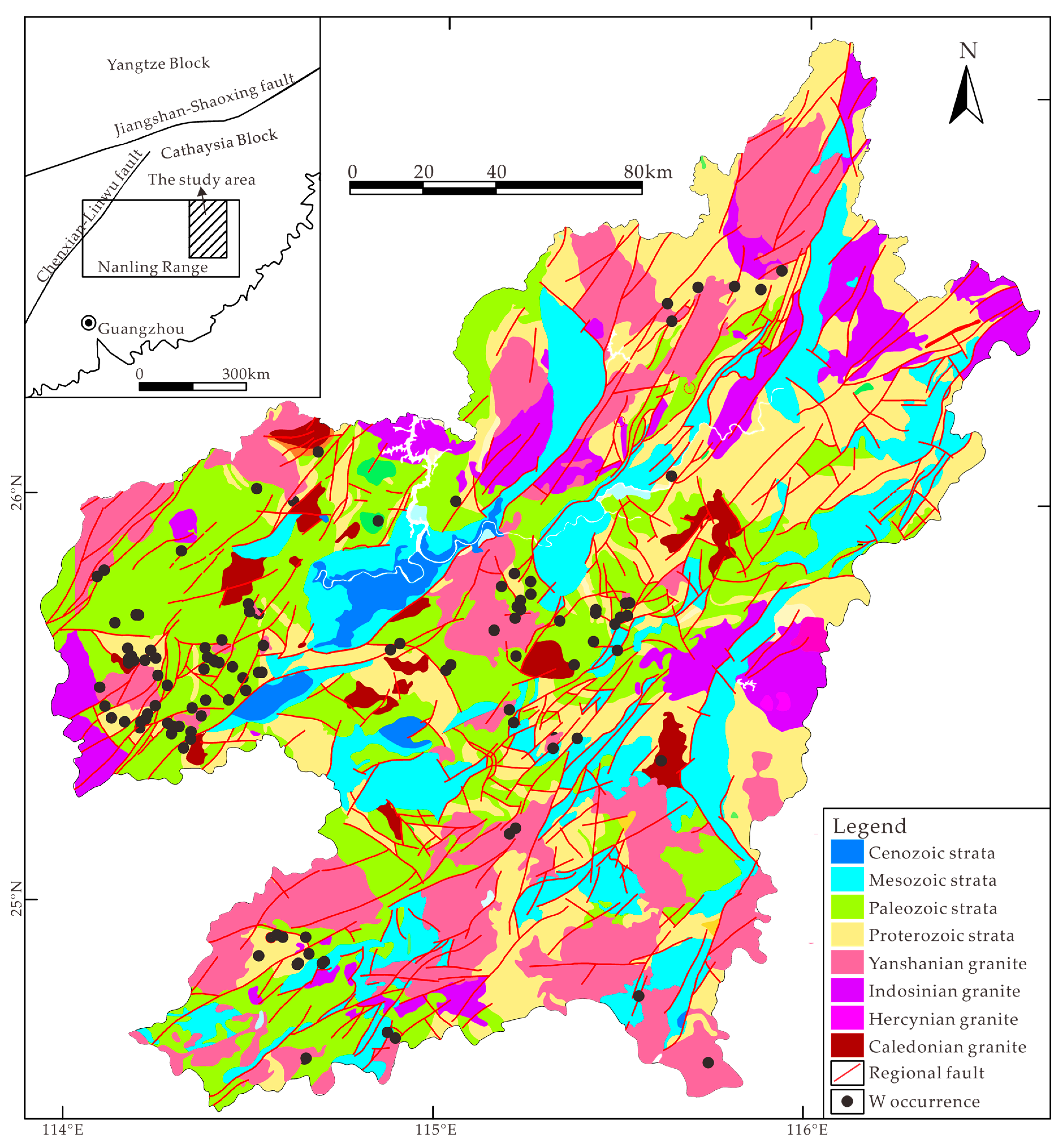
The southern Jiangxi Province, located in the central part of the Cathaysia block, pertains to the eastern segment of the giant Nanling metallogenic belt (Figure 1). The exposed sedimentary successions in this region include Neoproterozoic lower-greenschist facies clastic rocks, Paleozoic shallow marine carbonate and siliclastic rocks, Mesozoic strata consisting of volcaniclastics and terrigenous red-bed sandstone, and Cenozoic cover [39] (Figure 1). The tectonic framework of the study area is mainly controlled by three fault systems, trending approximately NE, EW, and NW, respectively (Figure 1). The study area has experienced four episodes of granitic magmatism, including Caledonian (Early to Middle Paleozoic), Hercynian (Late Paleozoic), Indosinian (Early Mesozoic), and Yanshanian (Late Mesozoic) [40], resulting in numerous intrusions with an outcropped area of approximately 14,000 km² (Figure 1). The granites exposed in this area are mainly biotite monzogranite, monzonite, and porphyritic monzogranite [38].

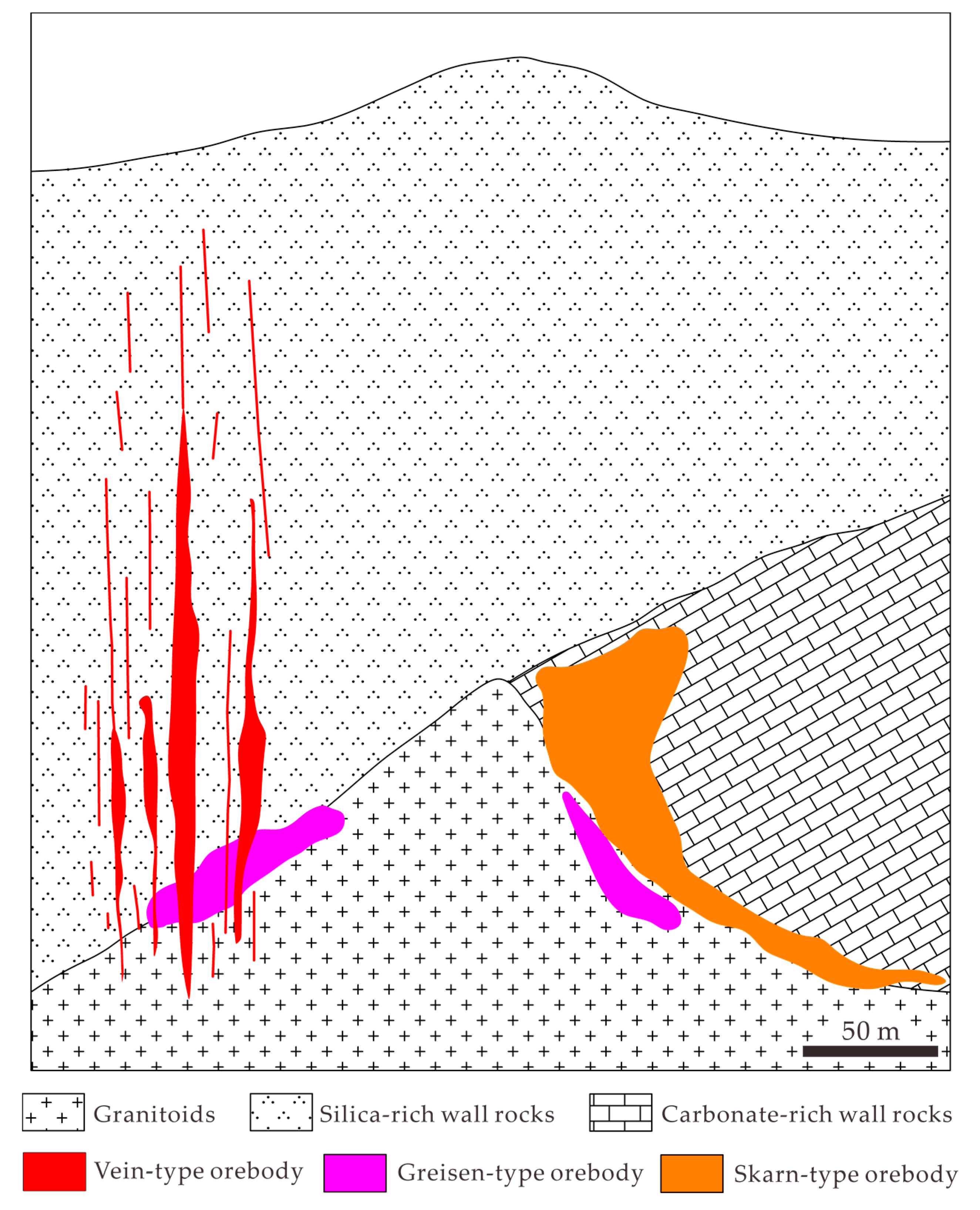
The densely distributed W deposits in this area are dominated by a quartz vein-type, with lesser amounts of skarn- and greisen-types [41]. The thickness of the mineralized veins ranges from millimeter-width veinlets to meter-width lodes [42] (Figure 2). The W mineralization of various types is spatially, temporally, and genetically related to Yanshanian granitic intrusions. All of the W deposits occur at the contacts between the intrusions and sedimentary wall rocks [42,43] (Figure 2). The detailed chronological studies show that the W deposits in this area formed in the late Jurassic (mainly 170–150 Ma), and there is no significant time difference (1–6 Ma) between the W orebodies and their proximal granitic intrusions [38,44]. The genetic models for W deposits in this area emphasize the close relationship of W mineralization and the evolution of Yanshanian granites [42,45,46]. The granitic magmas were derived from partial melting of the crust with the input of mafic materials, and then underwent significant differentiation and enrichment in W with abundant volatiles in the apical parts of magma chambers. The metalliferous fluids were exsolved from the melts as the magma was emplaced at a shallow level [42]. The greisen-, quartz vein-, and skarn-type mineralization were likely to form when the fluids successively encountered the granitic intrusions, clastic, and carbonate country rocks (Figure 2). These types of W mineralization belong to an integrated hydrothermal mineral system, and thus share the ore-forming components such as metal source and fluids pathways. W mineralization of these types can be predicted by the similar combination of evidential maps representing the above components. The regional fault systems are believed to exert a significant control on the Yanshanian tectono-magmatic activity and associated W mineralization. The emplacement of ore-related granitic magma was controlled by deep faults, especially those faults pertaining to the NE-NNE trending tectonic system which is interpreted to be formed in Yanshanian epoch. These provided pathways for the ascent of ore-related magma [47]. Secondary faults in the caprocks formed the transport networks for the metalliferous fluids, and intersections of these faults provided permeable space for trapping and focusing the fluids [47].

3. Methods

3.1. Random Forest (RF)

Random forest is an ensemble learning algorithm. This aggregates multiple decision trees to perform repeated predictions of the phenomenon represented by the training dataset [50]. Decision trees are used as base classifiers that constitute the “forest”. These trees are generated based on diverse training subsets. A sampling procedure known as “bootstrap aggregating” (also called “bagging” for short) is employed to generate training subsets by randomly sampling the original training dataset with a replacement (i.e., the chosen samples used for creating a tree are not deleted from the input dataset and can be selected again for the generation of the next tree) [5,51].

The trees grow by iteratively splitting the root nodes into binary leaf nodes. Such data splitting process in each internal node is repeated until a pre-specified stop condition is reached [28,51]. Unlike a standard decision tree, a subset of variables randomly selected from the input predictor variables are utilized as discriminative conditions at each node of the tree in the forest. The RF algorithm then searches through all the splits to find the optimal node which maximizes the purity of the resulting trees. The purity is a measurement of how often a randomly chosen sample from the input dataset would be correctly labelled if it was randomly labelled according to the distribution of labels in the subsets. The widely used Gini index (I_G) is employed in this study to calculate the information purity of leaf nodes when compared with that of their root nodes, which can be formulized as [52]:

$$I_G\left(f\right)={\displaystyle {\displaystyle \sum }_{i=1}^n}{f}_i\left(1-f_i\right)$$

(1)

where f_i is the probability of class i at node n. This is defined as:

$$f_i=\frac{m_j}{m}$$

(2)

where m_j is the number of samples belonging to class j, and m denotes the total number of samples in a specific node. The final predictive output of RF depends on the majority-voting of all the predictions of the decision trees.

The random scenarios of both sample selection and variable selection reduce the correlation among the individual trees and increase the diversity of the forest, which can effectively enhance the algorithm robustness and avoid overfitting [5,50].

3.2. Support Vector Machine (SVM)

The support vector machine was developed based on statistical learning and structural risk minimization [53]. This algorithm seeks to create a classifier that separates different classes using the widest decision boundaries, which was achieved by the generation of a hyperplane with maximum margins [54,55]. As this study focuses on binary classification (mineral occurrence or non-occurrence) based on integrated geological features that have complex nonlinear relationships, the nonlinear SVM algorithm used for binary classification is employed. This algorithm is described below.

Given a training dataset of ${\left\{x_i\right\}}_{i=1}^n$ with n predictor vectors, each vector is assigned with a label y_i. In this case, y_i = 1 represents mineral occurrence and y_i = −1 denotes non-occurrence. The input data are firstly mapped into a higher-dimensional space H through a mapping function Φ, where a hyperplane for separating two classes can be generated by the following equation [56]:

$$\{\begin{array}{c}\mathbf{w}\mathbf{\Phi }\left(x_i\right)+b\ge 1-{\xi }_i \mathrm{for} y_i=1 \\ \mathbf{w}\mathbf{\Phi }\left(x_i\right)+b\le -1+{\xi }_i \mathrm{for} y_i=-1 \\ {\xi }_i\ge 0, i=1,2,\dots ,\mathrm{n}\end{array}$$

(3)

where w and b are the weight vector and the bias term of the hyperplane; and ξ_i is the positive slack variable. According to the optimization theory, the problem of finding the optimal hyperplane is transformed into the problem of solving the following convex quadratic equation [26,56]:

$$\{\begin{array}{c}\mathrm{Minimize}: \frac{1}{2}{\Vert \mathbf{w}\Vert }^2\\ \mathrm{Subjected} \mathrm{to}: y_i\left(\mathbf{w}\mathbf{\Phi }\left(x_i\right)+b\right)\ge 1, i=1, 2, \dots , \mathrm{n}\end{array}$$

(4)

This optimization problem can be solved by the construction of a Lagrange function [26,57]:

$$L\left(\mathbf{w},\mathsf{\alpha }, b\right)=\frac{1}{2}{\Vert \mathbf{w}\Vert }^2-{\displaystyle {\displaystyle \sum }_{i=1}^n}{\alpha }_i{y}_i\left(\mathbf{w}\mathbf{\Phi }\left(x_i\right)+b\right)+{\displaystyle {\displaystyle \sum }_{i = 1}^n}{\alpha }_i$$

(5)

where α_i (i = 1, 2, …, n) is the Lagrange multiplier that is obtained by an optimization function [26,56,58]:

$$\{\begin{array}{l}\mathrm{Maximize}: {\displaystyle {\displaystyle \sum }_{i=1}^n}{\alpha }_i-\frac{1}{2}{\displaystyle {\displaystyle \sum }_{i=1}^n}{\displaystyle {\displaystyle \sum }_{j=1}^n}{\alpha }_i{\alpha }_j{y}_i{y}_j\mathbf{\Phi }\left(x_i\right)\mathbf{\Phi }\left(x_j\right)\\ \mathrm{Subjected} \mathrm{to}: {\displaystyle {\displaystyle \sum }_{i=0}^n}{\alpha }_i{y}_i=0, 0\le {\alpha }_i\le C, i=1,2,\dots ,\mathrm{n}\end{array}$$

(6)

where C is the penalty factor for misclassification error. A kernel function K can be defined here [57]:

$$K\left(x_i, x_j\right)=\mathbf{\Phi }\left(x_i\right)·\mathbf{\Phi }\left(x_j\right)$$

(7)

Some commonly used kernel functions include radial basis, linear, polynomial, and sigmoid. The radial basis function was employed in this study due to its low errors and simplicity of parameters in the practical application [58]:

$$K\left(x_i,x_j\right)=\exp \left(-\gamma \Vert x_i-x_j\Vert {}^2\right),\hspace{1em}\gamma >0$$

(8)

where γ is the width of radial basis function.

3.3. Artificial Neural Network (ANN)

ANN is a modelling method that is inspired by biological neural systems and simulates the pattern recognition ability of the human brain [59,60]. An artificial neuron is the functional unit that processes the received information. This is performed by using an activation function [61]. The sigmoid activation function employed in this study can be expressed as follows [62]:

$$f\left(x\right)=\frac{1}{1+Exp\left(-x\right)}$$

(9)

where x is the input data. The neurons are parallelly arranged in a group called “layer”. ANN have a typical multi-layered configuration consisting of an input layer, one or more hidden layers, and an output layer. The most commonly used neural network is feed-forward network and is employed in this paper. In this neural network, the neurons of different layers are fully interconnected to each other, but the information is unidirectional starting from the input layer through hidden layers to the output layer [5,60]. The information propagation is performed by assigning initialized weights to the connections of different neurons, which can be formulized as [5]:

$$y_j=f({\displaystyle \sum }_i{w}_{ji}{x}_i+b_j)$$

(10)

where w_ji is the weight that connects neuron i in the previous layer to neuron j, and b_j is the bias term of neuron j, while f is the activation function.

The back-propagation procedure is utilized to enhance the learning capability of ANN. This procedure computes the output error between the predicted value and real target value, then feeds it back to the ANN, and then the ANN tunes the weights and biases in the network to minimize the output error [60]. The extent of weight update is controlled by a learning rate. Such back-propagation processes are repeated until a pre-specified accuracy or the maximum number of iterations is reached.

3.4. Convolutional Neural Network (CNN)

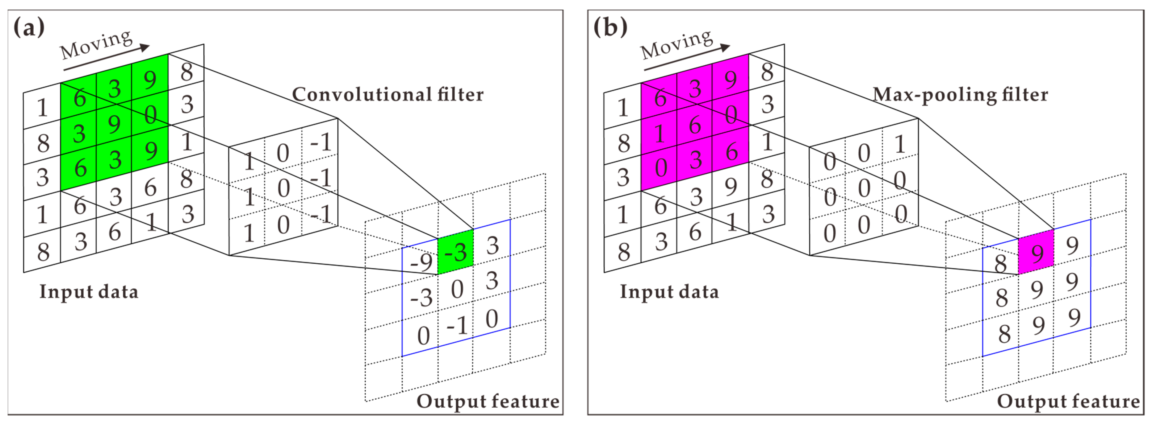
CNN is a class of deep learning neural network that basically consists of an input layer, one or more convolutional layers, pooling layers and fully connected layers, and an output layer. The input data, denoted as X = (x₁, x₂, …, x_n), are firstly given to a convolutional layer. The convolutional layer employs a randomly initialized filter (also called kernel) to perform a convolutional operation. Figure 3a shows an example of a convolution, where a convolutional filter is moved across the whole input dataset, and the dot products between the entries of the filter and the input data are calculated, resulting in a new feature dataset (referred to as a feature map). The use of different kernels (denoted as Σ_i) produces multiple convolutional results, based on which set of new feature maps is generated to provide different representations of the input vectors in a hierarchical manner, which can be expressed as [63]:

$$F_i=\left(f_1,f_2,\dots ,f_n\right)=g\left(X·{\mathsf{\Sigma }}_i\right)$$

(11)

where g is an activation function used for nonlinear amplification of convolutional results [64]. The rectified linear unit (ReLU) function is the most commonly used in CNN, which can be formulized as:

$$g\left(x\right)=\max \left(0,x\right)$$

(12)

The feature maps generated by one or more convolutional layers are then sent to a pooling layer. Pooling is also a filter-based operation that uses a moving filter to extract the maximum (max-pooling) or average (average-pooling) value of the data overlapped by the filter, as shown in Figure 3b. The max-pooling is employed in this study. The pooling layers are used for a down-sampling process to reduce the dimensions of the network that assist in reducing computational cost and controlling overfitting problems [63]. In this way, the input data are propagated through successive convolutional and pooling layers to extract features [63]. The extracted feature maps are sent to several fully connected layers, which can be considered as the dependent ANN described above. The output of the fully connected layers is sent to the last layer which utilizes a softmax activation function to calculate the predictive probability of all classes by the following formula [63]:

$$P\left(y=j|x\right)=\frac{\exp \left(w_{j}x+b_j\right)}{{{\displaystyle \sum }}_{i=1}^2\exp \left(w_{i}x+b_i\right)}$$

(13)

where y denotes the predicted class, and w and b are weight and bias terms for the corresponding class, respectively.

In MPM, the input data of machine learning can be considered as a picture where each pixel represents a measurement of a specific feature. Therefore, each grid cell is represented by a column vector with a length determined by the number of evidential features. In this regard, the CNN with one-dimensional data representation that has a typical architecture illustrated in Figure 4, was employed in this study. Assuming that there are n evidential features in the input dataset, a convolutional layer employing N filter with a size of (n × 1) results in N new feature vectors with a length of (m − n + 1). The output of the convolutional layer is then set a pooling layer using a filter of (a × 1), resulting in N feature maps with a size of [(m − n − a + 2) × 1]. After one or more convolution-pooling operations, the output feature maps are input into a fully connected neural network with x neurons. Finally, the last fully connected layer uses a softmax function to yield the predictive probability and outputs a binary prediction.

4. Datasets and Application

Preparation of input data (including predictor and target variables) is the first and an important step of MPM. The integration of multi-source predictor variables and generation of input datasets were implemented by using ESRI’s ArcGIS software (Version 10.2, Environmental Systems Research Institute, Redlands, CA, USA). The application of ML-based modelling, including model training and assessment, was carried out in a RapidMiner Studio (Version 9.3, RapidMiner, Inc., Boston, MA, USA). This software provides numerous practical modelling toolkits and embeds an abundant source of machine learning algorithms.

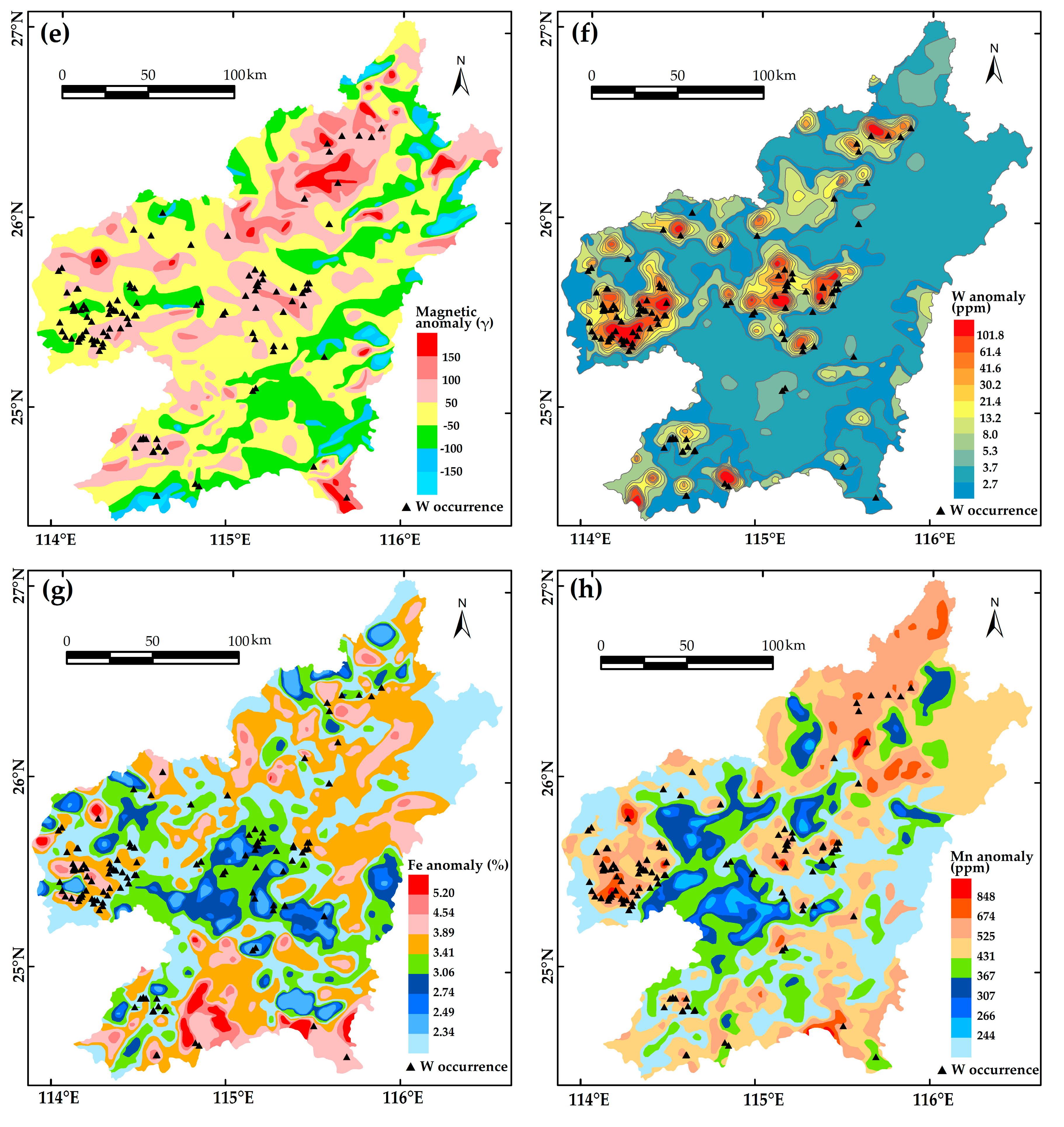
4.1. Predictor Variables

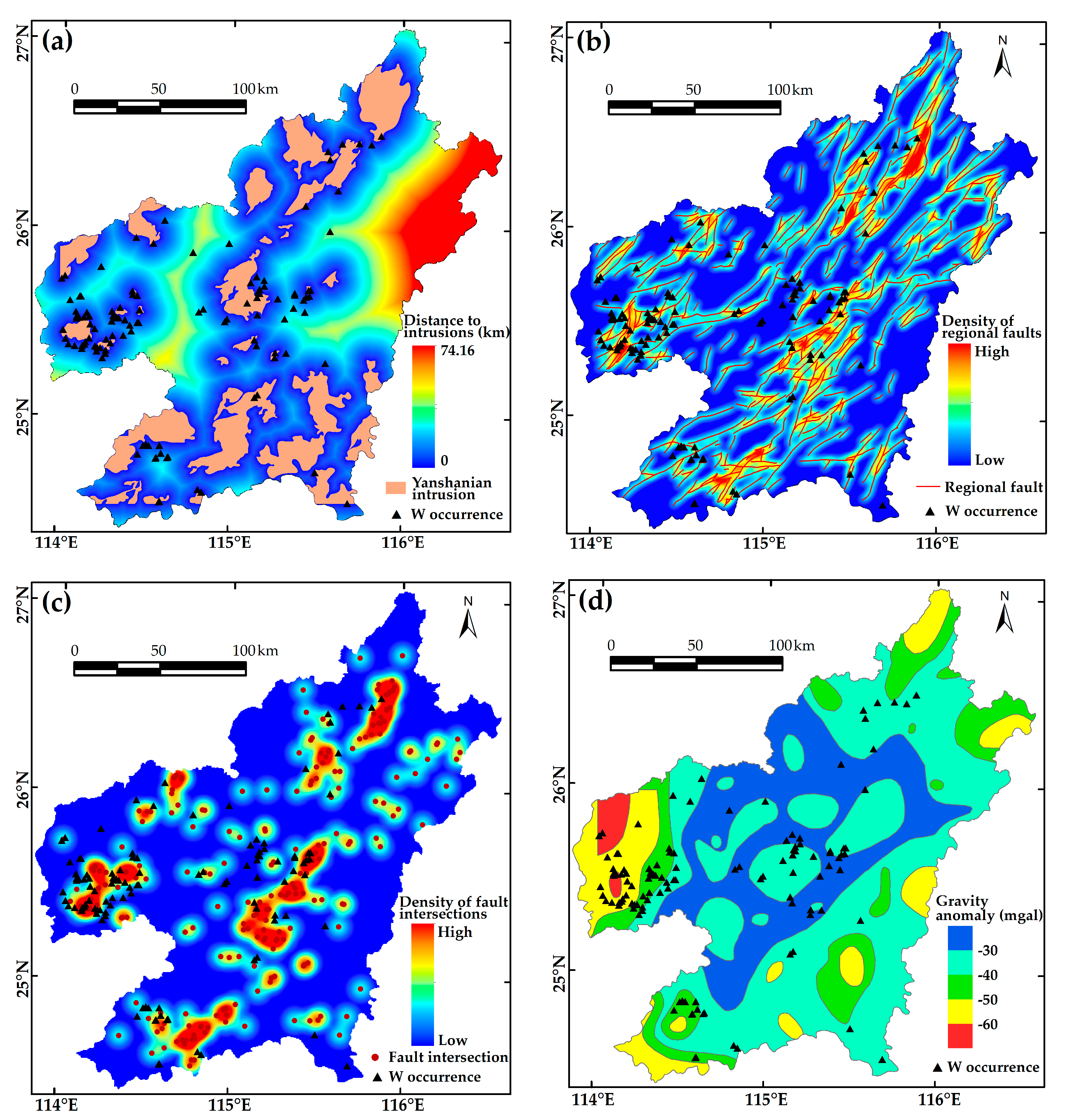
Predictor variables are used as decisive conditions for predicting mineral potential. The reliable variables should be guided by the understanding of W mineral system. According to the genetic model and controlling factors of W mineralization described in Section 2, and based on the collection of publicly accessible data, we utilized eight evidential maps as predictor variables involving geological, geophysical, and geochemical information.

Geological data originated from an online database of the China Geological Survey based on decades of regional investigations [49]. Proximity to outcropped Yanshanian intrusions was employed as an evidential map representing the source component of the ore-forming system (Figure 5a). According to a spatial analysis conducted in this area [65], NE- and EW- trending regional faults exhibit a positive relationship with W occurrences, whereas NW-trending faults were likely formed post-mineralization, and, show no obvious spatial association with mineral occurrences. Therefore, density maps of NE- and EW- trending faults and their intersections were used as evidences to represent structural controls on mineralization (Figure 5b,c). Geophysical anomalies can provide information about subsurface bodies, such as the intrusive rocks in the area. Thus, geophysical data, including gravity and magnetic [66], were utilized to recognize the occurrence of ore-related intrusive rocks at depth (Figure 5d,e). Geochemical anomalies of mineralized elements are direction indications for the targeted deposits. As W, Mn, and Fe are the most important constituents of wolframite ((Fe,Mn)WO₄) that dominates the ores in this area, geochemical anomalies in these elements, extracted from stream sediment geochemical data of Nanling Range [67], were employed as evidential maps (Figure 5f–h). The data were derived from China’s National Geochemical Mapping Project with sampling density of one sample per km² [68]. W was analyzed by the polarography method, and Mn and Fe were analyzed by the X-ray fluorescence method [69].

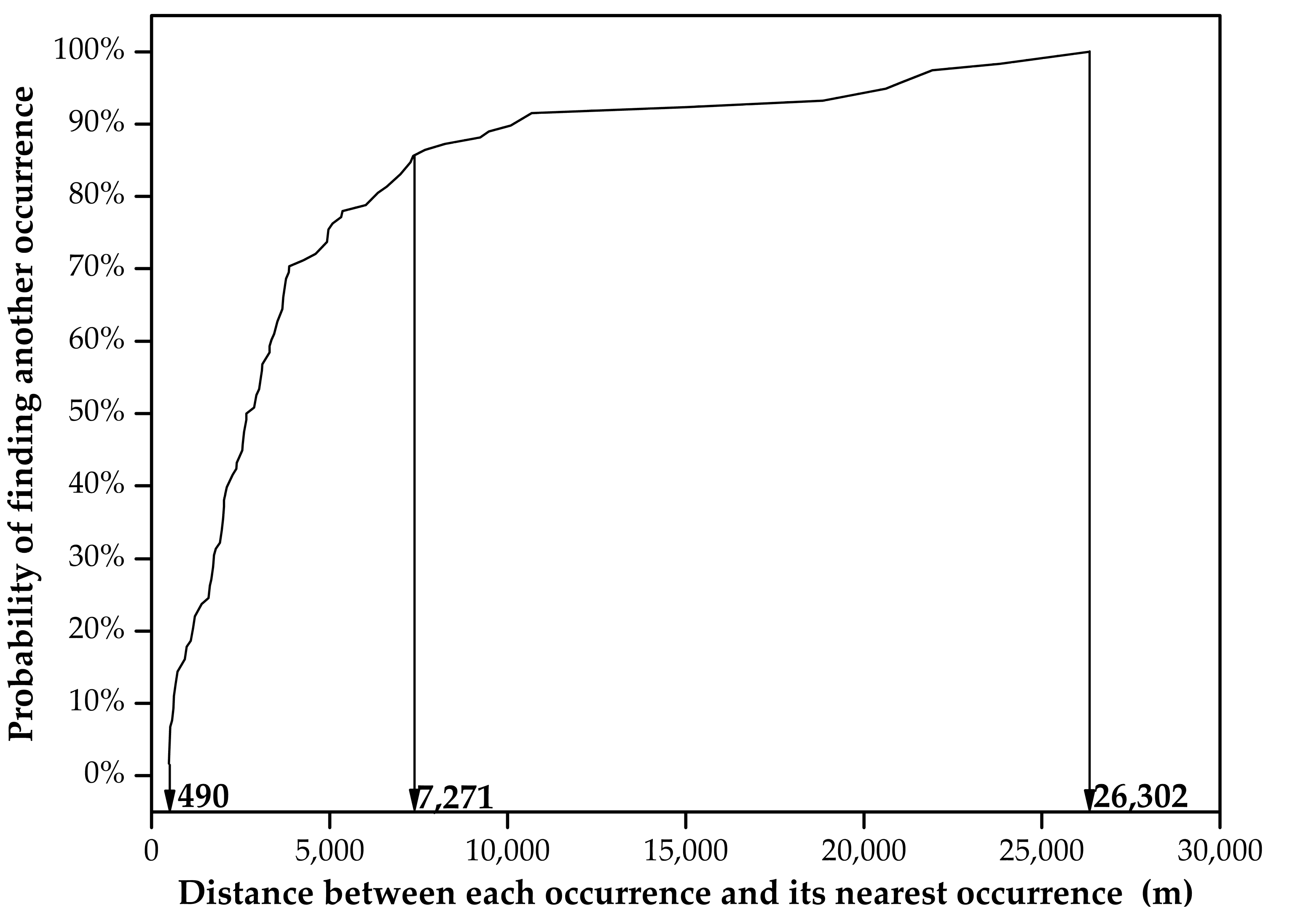
After preparation of the evidential maps, they were transformed into raster maps where each cell has a numerical representation of the evidential features. The cell size was determined based on an objective scenario proposed by Carranza [70]. Considering the scarcity of mineral occurrences, the cell grid should ensure that any single cell contains only one mineral occurrence. The neighboring distance analysis can help provide a reference range of cell size. The distances between each known occurrence and its nearest neighboring occurrence were calculated and statistically plotted (Figure 6). It can be observed that the minimum distance of any two nearest occurrences is 490 m. This sets an upper limit of the cell size. The lower limit of cell size R_s can be calculated by an empirical formula [71]:

$$R_s=M_s\times 0.00025$$

(14)

where M_s denotes the map scale. The largest scale of the evidential maps employed in this study is 1:300,000. This indicates that the lower limit of the cell size should be 75 m. A cell size of 450 m was selected to generate a raster gird containing 195,174 cells. Each cell has a combination of eight feature values indicative of geological, geophysical, and geochemical evidence.

4.2. Target Variable

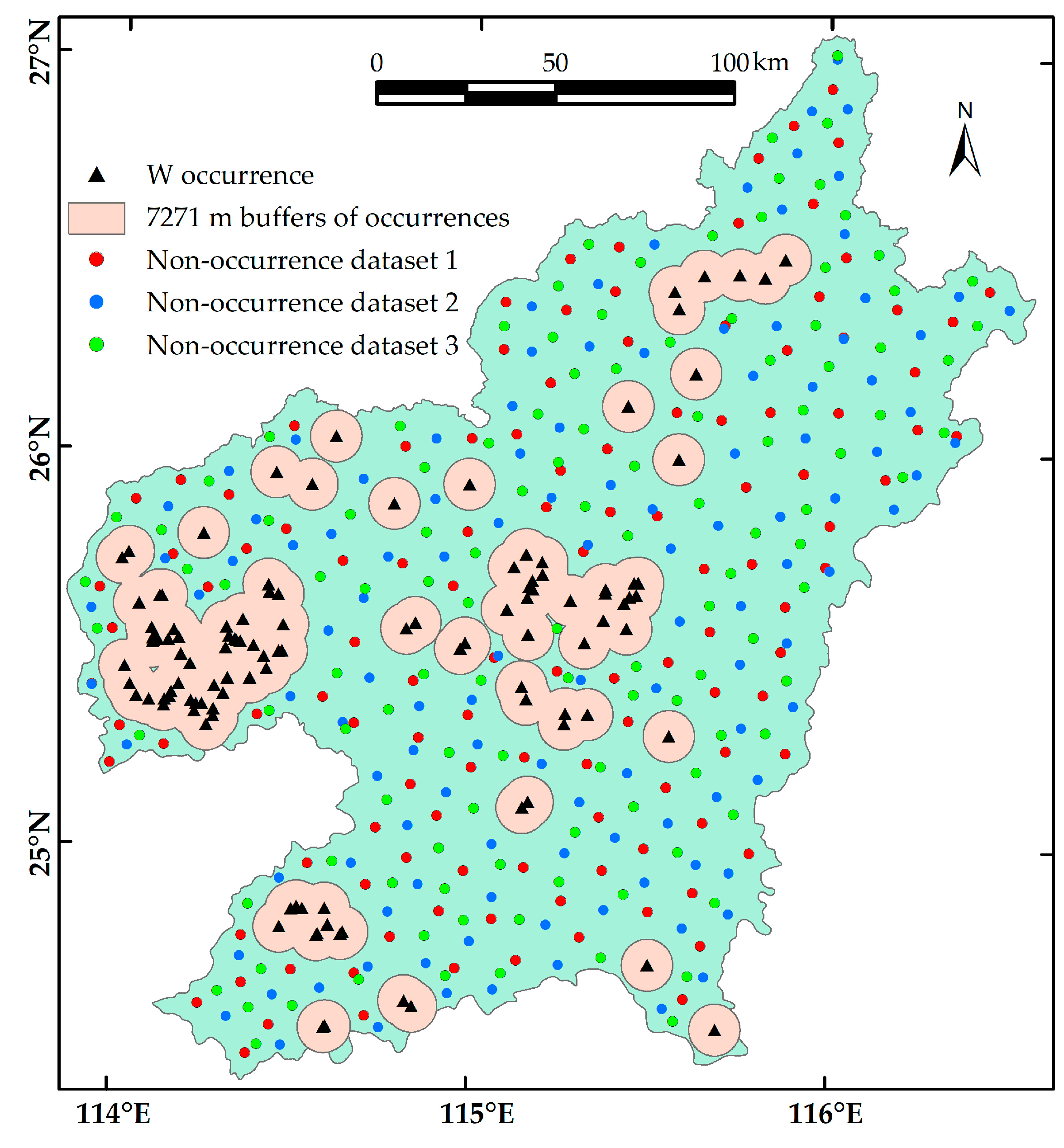
The target variables, including mineral occurrences and non-occurrence locations, are used as training and validation samples for a supervised predictive modelling. The mineral occurrences were derived from the online database of China Geological Survey [49]. The non-occurrence locations were selected according to the scenario proposed by Carranza and Zuo [58,72]: (i) The quantity of non-occurrence samples should be equal to that of mineral occurrences, so that the ratio of positive and negative samples in the training and validation datasets would be balanced. (ii) The non-occurrence locations should be distal enough to any known occurrence. Regions proximal to the existing mineral occurrences are likely to have similar ore-forming conditions. The neighboring distance analysis of mineral occurrences can be used to define the distance beyond which the non-occurrence locations should be selected (Figure 6). It can be observed that the maximum distance between any two occurrences is 26,302 m. There is 100% probability to find another occurrence within 26,302 m of any occurrence. Non-occurrence locations should be selected beyond the 26,302 m buffered range of mineral occurrences. However, few locations can be selected in this range. Instead, 7271 m was selected as a buffered range where there is 85% probability to find a neighboring occurrence next to any existing occurrence, and the non-occurrence samples should be selected outside the buffered areas (Figure 7). (iii) Mineral occurrences in a specific area generally have a spatially clustered distribution (Figure 7), because they are products of rare events and non-random ore-forming processes. In contrary, non-occurrence locations should be spatially randomly distributed as they resulted from common geological processes.

Although the above criteria used for selecting non-occurrence locations are objective based on statistical data and distribution of mineral occurrences, manual selection may still result in some uncertainty in non-occurrence datasets with respect to the mixture of some concealed mineral occurrences. This would greatly influence the reliability of modelling results [58]. To reduce the effect of falsely negative samples, three non-occurrence datasets were generated. Each consists of 118 non-occurrence samples that were selected according to the random scenario mentioned above (Figure 7), resulting in three datasets of target variables. The three labelled datasets were then randomly divided into two parts, including 70% of labelled samples serving as training dataset and the other labelled samples then used as validation dataset.

4.3. Model Training

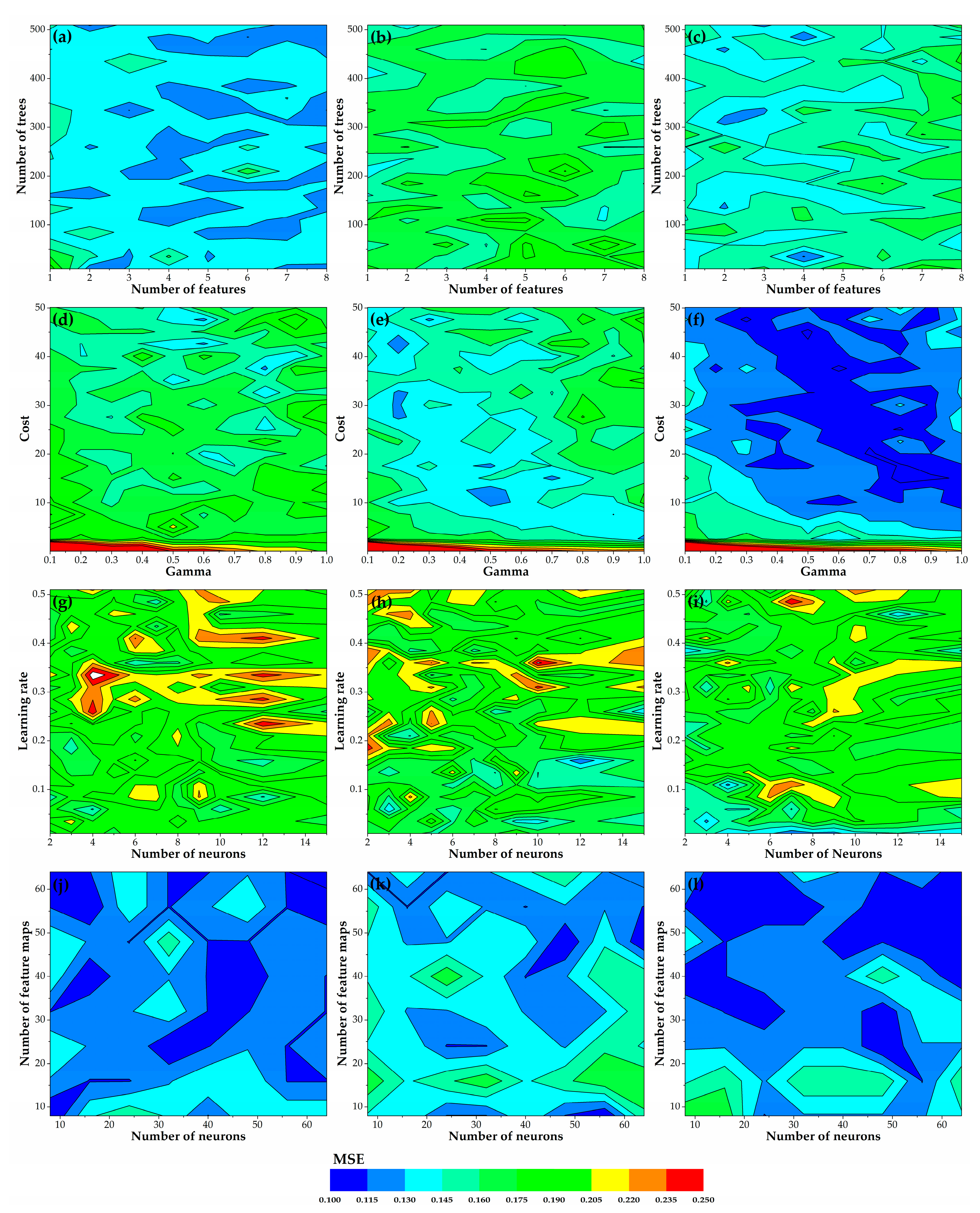
After the preparation of input data, ML models were generated by training processes. These mainly involved the determination of key parameters used for the ML models. It is difficult to specify a priori suitable configuration of parameters in data-driven modelling. The optimal parameters for individual ML models vary with specific input datasets and different application backgrounds. There is no universally empirical rule for determining these parameters. In this regard, a highly objective trial-and-error procedure is invariably needed to obtain the optimal parameters. A grid search method was employed to conduct this procedure.

Table 1. Parameters used for training machine learning models.

Model	Parameter	Description	Reference Range
RF	Number of trees	Number of trees in the random forest	10–500
	Number of features	Number of features used for developing each tree	1–8
SVM	Gamma	A width parameter of RBF that determines the influencing range of each support vector	0.1–1
	Cost	Penalty factor for misclassification error	0.1–50
ANN	Number of neurons	Number of neurons in the hidden layer	2–15
	Learning rate	Change rate of weight in the training process	0.1–0.5
CNN	Number of feature maps	Number of convolutional filters used for generating new feature maps	8–64
	Number of neurons	Number of neurons used in the fully connected layers	8–64

lists the key ML parameters and their reference ranges of values suggested by previous studies [5,28,32,55,62,73,74]. The possible combinations of parameters used for training individual ML models were obtained by searching the reference ranges of values with a specified step length. A 10-fold cross-validation procedure was then implemented to assess the classification performance of the trained ML models using the possible combinations of parameters. In this procedure, the input training datasets were randomly divided into 10 subsets with equal size of these, nine subsets were utilized to train predictive models and the remaining one was employed as a test dataset to calculate the classification errors. This procedure was repeated 10 times until each subset had been used once as the test dataset (c.f., [75]). The mean square error (MSE) was utilized to assess the classification performance of trained models. This can be calculated by the following formula:

$$MSE=\frac{1}{N}{\displaystyle {\displaystyle \sum }_{i=1}^N}{\left(\widehat{y_i}-y_i\right)}^2$$

(15)

where N is the number of samples in the test dataset; $\widehat{y_i}$ denotes the predicted result of each sample (i.e., 1 for mineral occurrence and 0 for non-occurrence); y_i denotes the true value of each sample. The combination of parameters that trains the best model with the lowest MSE was determined as the optimum model configuration.

4.4. Model Assessment

The comprehensive performance of trained ML models, including classification accuracy, predictive capability, and geological interpretability, was assessed by a series of quantitative measurements.

The classification accuracy of a predictive model can be evaluated by the confusion matrix, in which the classification result of a sample can be categorized into the following four situations: (i) A mineral occurrence is correctly classified as an occurrence, referred to as true positive sample or TP; (ii) a mineral occurrence is incorrectly classified as a non-occurrence, referred to as false negative sample or FN; (iii) a non-occurrence sample is correctly classified into non-occurrence class, referred to as true negative sample or TN; and (iv) a non-occurrence sample is incorrectly classified as a mineral occurrence, referred to as false positive sample or FP. Based on the confusion matrix, a set of statistical indices can be calculated to assess the classification performance of the ML models, which can be formulized as [76,77]:

$$Sensitivity=\frac{TP}{TP+FN}$$

(16)

$$Specificity=\frac{TN}{TN+FP}$$

(17)

$$Positive predictive value=\frac{TP}{TP+FP}$$

(18)

$$Negative predictive value=\frac{TN}{TN+FN}$$

(19)

$$Accuracy=\frac{TP+TN}{TP+TN+FP+FN}$$

(20)

The overall predictive performance of ML models was assessed by the receiver operating characteristic (ROC) curve and success-rate curve. These curves are graphical representations of model precision with respect to the variation of discrimination thresholds that define the predictive results of a binary classification system [78,79]. More specifically, a cell with a probability value greater or lower than the discrimination threshold was predicted as “mineral occurrence” or “non-occurrence”, based on which the sensitivity and specificity were calculated. The prospective regions were delimited by those cells classified as mineral occurrence. By gradually decreasing the discrimination thresholds, the ROC curve was generated by plotting the corresponding true positive rate (also known as sensitivity that denotes the ratio of correctly classified positive samples) on the y-axis against false positive rate (the ratio of incorrectly classified negative samples, given by (1-specificity)) on the x-axis, while the success-rate curve was created by plotting the percentage of mineral occurrences included in the prospective regions against the area percentage of prospective regions. In addition, the area under the ROC curve (AUC) was utilized as a quantitative measurement of the predictive performance of ML models.

Information gain (IG) was used in this contribution to estimate the influence of input predictor variables on the predictive models. This helps to interpret the relative importance of the related geological features and thus can validate the reliability of the predictions. The information gain for a specific predictor variable corresponding to the output classification result Y can be obtained by [80]:

$$IG\left(Y,F_i\right)=H\left(Y\right)-H\left(Y|F_i\right)$$

(21)

where H(Y) is the entropy value of Y that used to describe unpredictability of being classified into Y, and H(Y|F_i) is the modified entropy value of Y after being associated with a given evidential feature F_i (see [80] for detail).

5. Results and Discussion

5.1. Model Configulartion and Its Influence on Classification Precision

For a data-driven predictive modelling, model configuration greatly influences the accuracy of predictions. MSE obtained from the 10-fold cross-validation is employed in this study to assess the classification precision in the training process. Figure 8 shows the variations of MSE with varying combinations of ML parameters and different datasets. Although individual ML models trained by the three datasets achieve different levels of classification precision, they exhibit similar variation patterns of MSE with respect to changes of the specific parameter. In general, RF and CNN models present a more accurate and stable performance than the other two models, yielding predictions with MSE lower than 0.19 and responding less sensitively to parameter changes. The SVM models produce poor classification results with low cost value (<2.5), and the ANN models yield the most complex and inaccurate predictions in the training process according to variation patterns of MSE, especially when the learning rate is greater than 0.2.

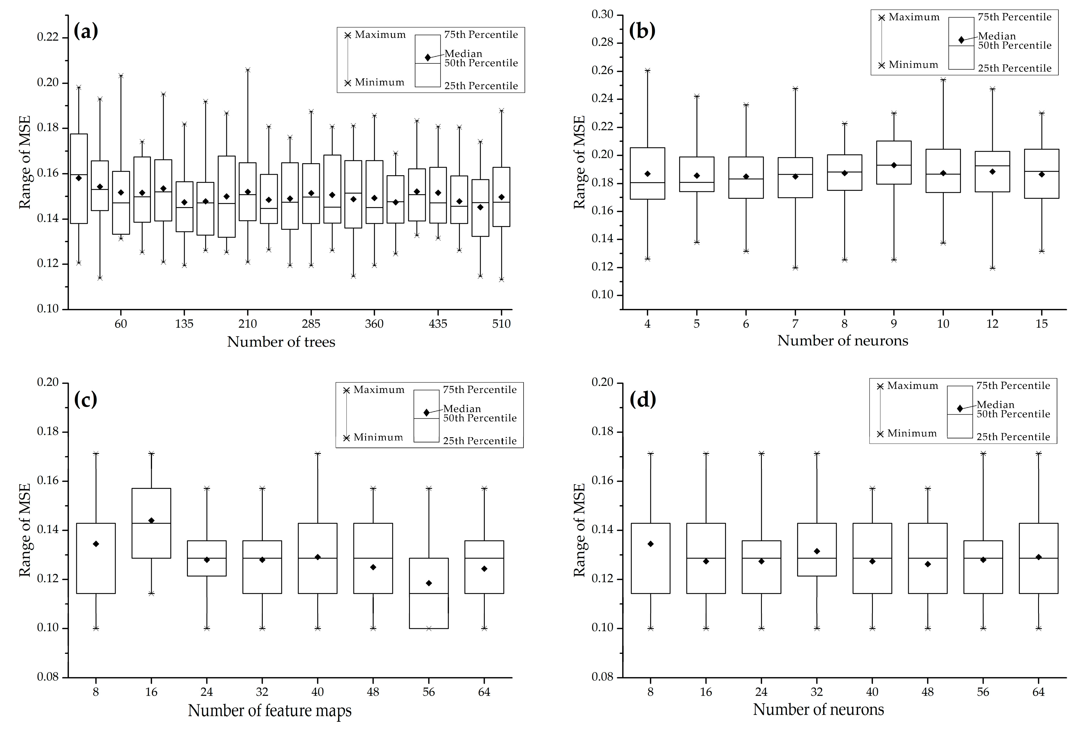
Among all the ML parameters, some are related to model architecture, including number of trees in RF, number of neurons in ANN, as well as number of feature maps and number of neurons in CNN, define the complexity of the corresponding models. It is commonly recognized in many research fields that elaborate ML models tend to yield more accurate predictions [29,32,81]. However, in this study regarding prospectivity modelling, a statistical analysis of MSE results with an increment of architecture-related parameters was conducted. The results indicate that complex architectures of models do not lead to better performance in the prospectivity modelling of the study area, as shown in Figure 9. As the relevant parameters increase, all statistical indices, especially the lowest MSE and average MSE used for evaluating the classification error, do not exhibit an obvious decreasing trend. Conversely, the increasing number of trees, neurons, and feature maps remarkably increase the computing cost. It is implied that elaborate architectures of ML models are not necessarily needed in the modelling processes presented here. This implication is in accord with some previous studies [5,24] that also reveal complex models did not necessarily result in more accurate predictions. These results may be attributed to the small size of training datasets that usually consist of dozens of mineral deposit and non-deposit locations. Training models with such limited datasets may easily achieve the desired precision, whereas complex architectures and excessive training may produce over-fitting errors.

5.2. Model Assessment and Selection of Prospectivity Map

The ML models trained by the optimal combinations of parameters output the prediction at each cell that is represented by a floating probability value ranging from 0 to 1 (Figure 10). The ML algorithms label those cells with probability values greater than 0.5 as prospective areas that potentially contain a mineral occurrence. Other cells are marked as barren regions without sufficient prospecting potential. According to such classification scenario, the confusion matrices of validation datasets for the four ML methods are generated and listed in

Table 2. Confusion matrices of machine learning models in different validation datasets.

Model	Predictive Class	Dataset 1		Dataset 2		Dataset 3
		True Deposit	True Non-Deposit	True Deposit	True Non-Deposit	True Deposit	True Non-Deposit
RF	Predicted deposit	30	3	28	2	29	3
	Predicted non-deposit	5	32	7	33	6	32
SVM	Predicted deposit	28	2	28	3	26	2
	Predicted non-deposit	7	33	7	32	9	33
ANN	Predicted deposit	27	3	28	3	27	2
	Predicted non-deposit	8	32	7	32	8	33
CNN	Predicted deposit	30	0	31	2	31	1
	Predicted non-deposit	5	35	4	33	4	34

, based on which the accuracy of binary classification is quantitatively measured by various statistical indices, as listed in

Table 3. Classification performance of machine learning models.

Model	Dataset	Sensitivity	Specificity	Positive Predictive Rate	Negative Predictive Rate	Accuracy
RF	Dataset 1	85.71%	91.43%	90.91%	86.49%	88.57%
	Dataset 2	80.00%	94.29%	93.33%	82.50%	87.14%
	Dataset 3	82.86%	91.43%	90.63%	84.21%	87.14%
	Average	82.86%	92.38%	91.62%	84.40%	87.62%
SVM	Dataset 1	80.00%	94.29%	93.33%	82.50%	87.14%
	Dataset 2	80.00%	91.43%	90.32%	82.05%	85.71%
	Dataset 3	74.29%	94.29%	92.86%	78.57%	84.29%
	Average	78.10%	93.34%	92.17%	81.04%	85.71%
ANN	Dataset 1	77.14%	91.43%	90.00%	80.00%	84.29%
	Dataset 2	80.00%	91.43%	90.32%	82.05%	85.71%
	Dataset 3	77.14%	94.29%	93.10%	80.49%	85.71%
	Average	78.09%	92.38%	91.14%	80.85%	85.24%
CNN	Dataset 1	85.71%	100.00%	100.00%	87.50%	92.86%
	Dataset 2	88.57%	94.29%	93.94%	89.19%	91.43%
	Dataset 3	88.57%	97.14%	96.88%	89.47%	92.86%
	Average	87.62%	97.14%	96.94%	88.72%	92.38%

. It can be seen that individual models exhibit different performances in different datasets and in different indices. In general, the CNN model achieves the greatest performance both in the overall accuracy and in predicting positive and negative samples, followed by the RF and SVM models, whereas the ANN model produces relatively worse predictions. Specifically, the CNN model is the most sensitive that correctly identifies 87.62% of deposit locations in all the three datasets, followed by the RF model (82.86%). The sensitivity values of the SVM and ANN models are both lower than 80%. The CNN model has a specificity of 97.14%, indicating that 97.14% of non-occurrence cells are correctly classified as barren regions. The rest of the models also achieve very high values of specificity: 93.34%, 92.38%, and 92.38% for the SVM, RF, and ANN models, respectively. All four models have high positive predictive values greater than 91%, meaning that more than 91% of the predicted prospective cells actually contain W occurrences. The ANN model yields the lowest negative predictive rate (80.85%), indicating that 80.85% of predicted non-occurrence cells are true non-occurrence locations. In contrast, the CNN model achieves the highest negative predictive rate (88.72%), followed by the RF (84.40%) and SVM (81.04%) models. The CNN model achieves the highest overall accuracy of 92.38%, indicating 92.38% of all samples are correctly classified, followed by the RF model (87.62%), whereas the SVM (85.71%) and ANN (85.24%) models produce relatively low values of classification accuracy.

All the ML models can correctly identify most known occurrences (>78%) in the prospective areas defined by the default classification scenario (i.e., probability > 0.5). However, for “real world” mineral exploration, it is unrealistic to explore all these “prospective areas” due to the expense of exploration. Therefore, target regions ideally possess the highest confidence over the smallest area. The delineation of high-confidence zones and predictive efficiency of the models are essential for exploration applications and thus need to be effectively assessed.

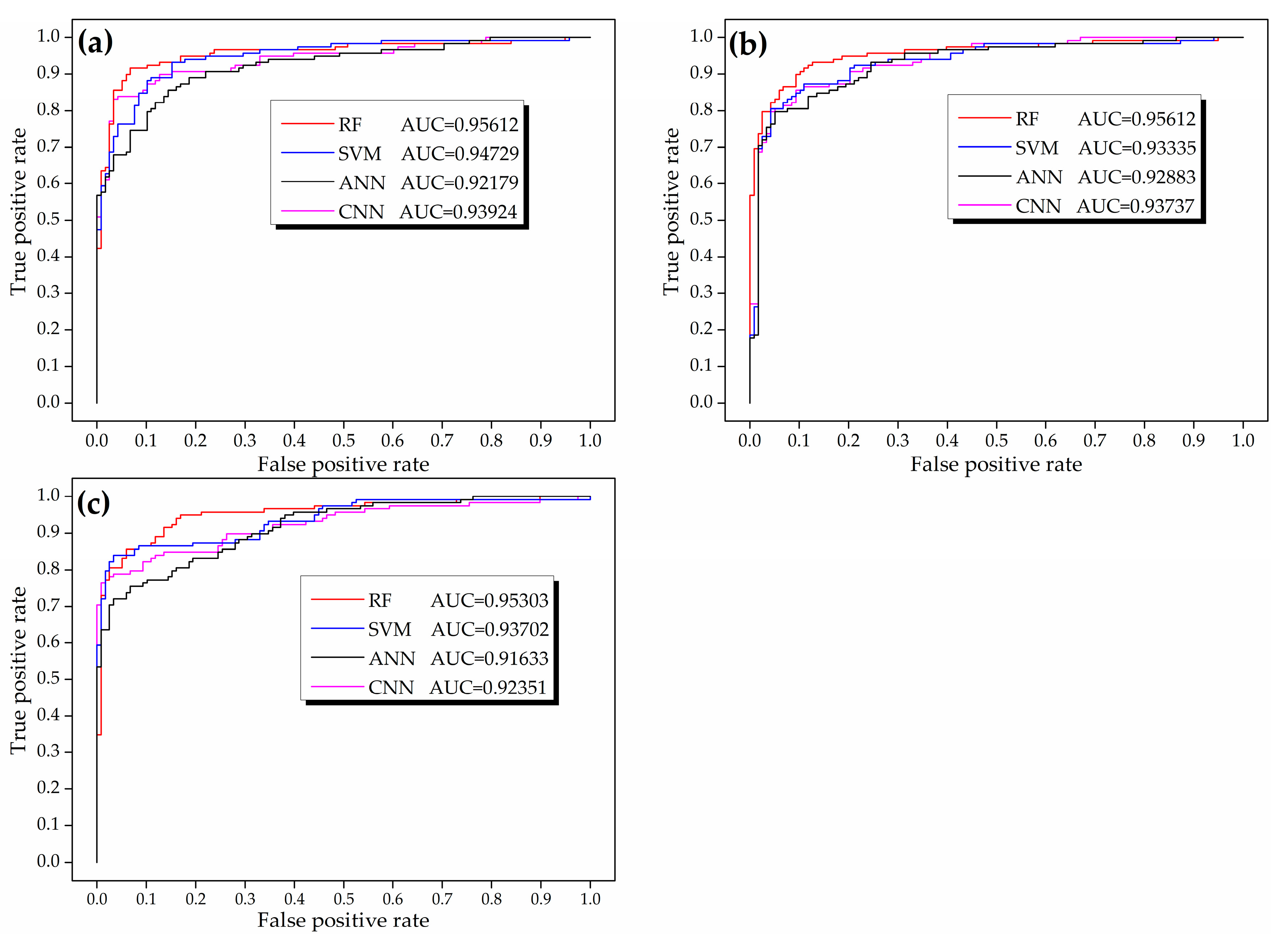
The predictive performance of high-probability zones can be evaluated by the ROC curve. Classification results of predictions are judged by varying discriminative thresholds from high to low probability values. In the ideal situation that all the occurrence samples have higher probability than the non-occurrence ones, the ROC curve is a y = 1 straight line with the highest AUC of 1. A non-occurrence cell with high probability or an occurrence cell with low probability would make the ROC curve deviate from the y = 1 curve and decrease the AUC value. The ROC curves of the four ML models trained by different input datasets are exhibited in Figure 11. It is suggested that the closer a ROC curve is towards the upper left corner, the closer it is towards the y = 1 curve, and the better the model performs. The ROC curve of the RF model is the closest to the top left corner in all cases, having the highest AUC values that are greater than 0.95. The SVM and CNN models show comparable performance with secondary highest AUC values, whereas the ANN model performs the weakest predictive capability in the assessment of ROC curves.

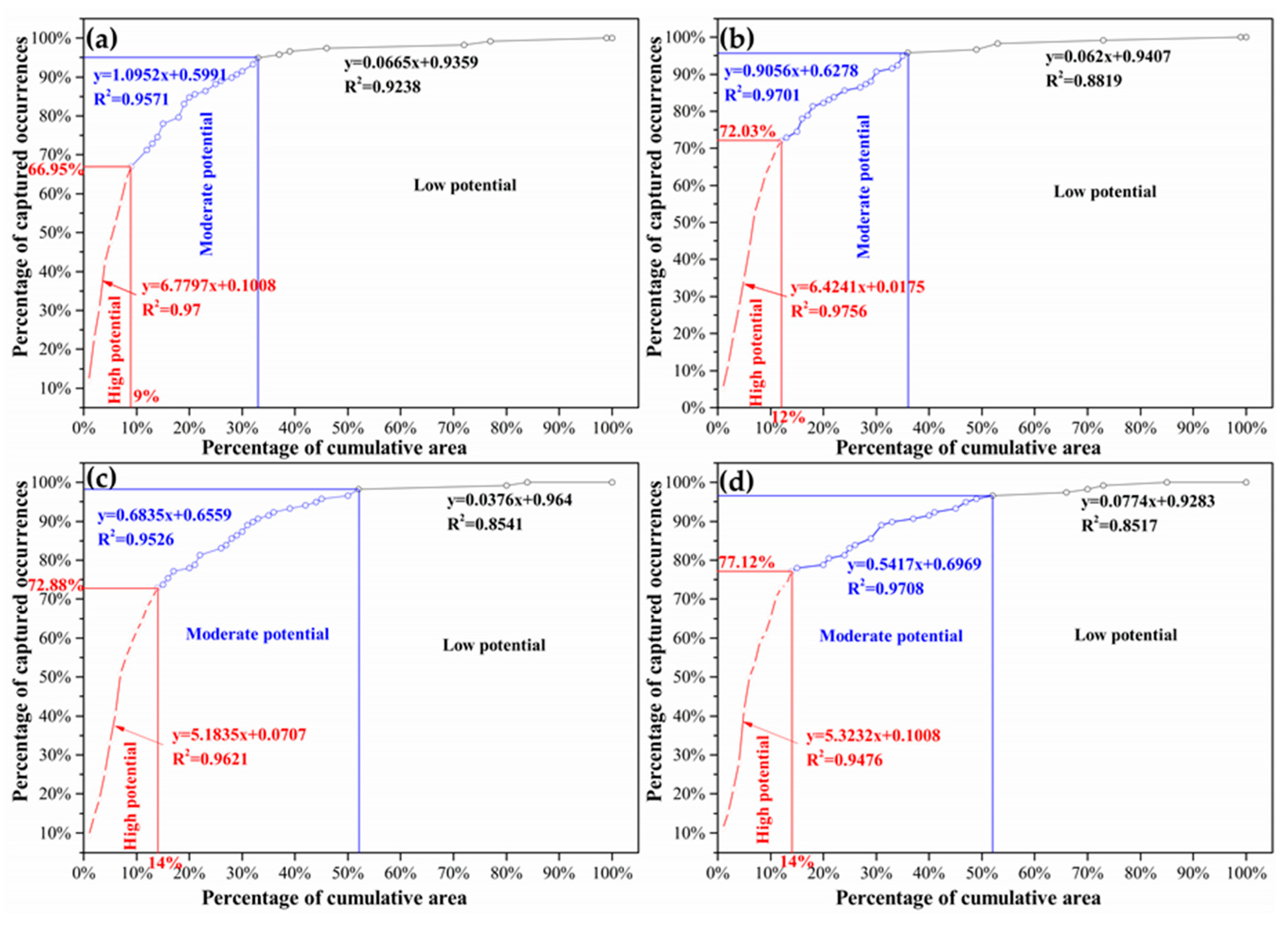
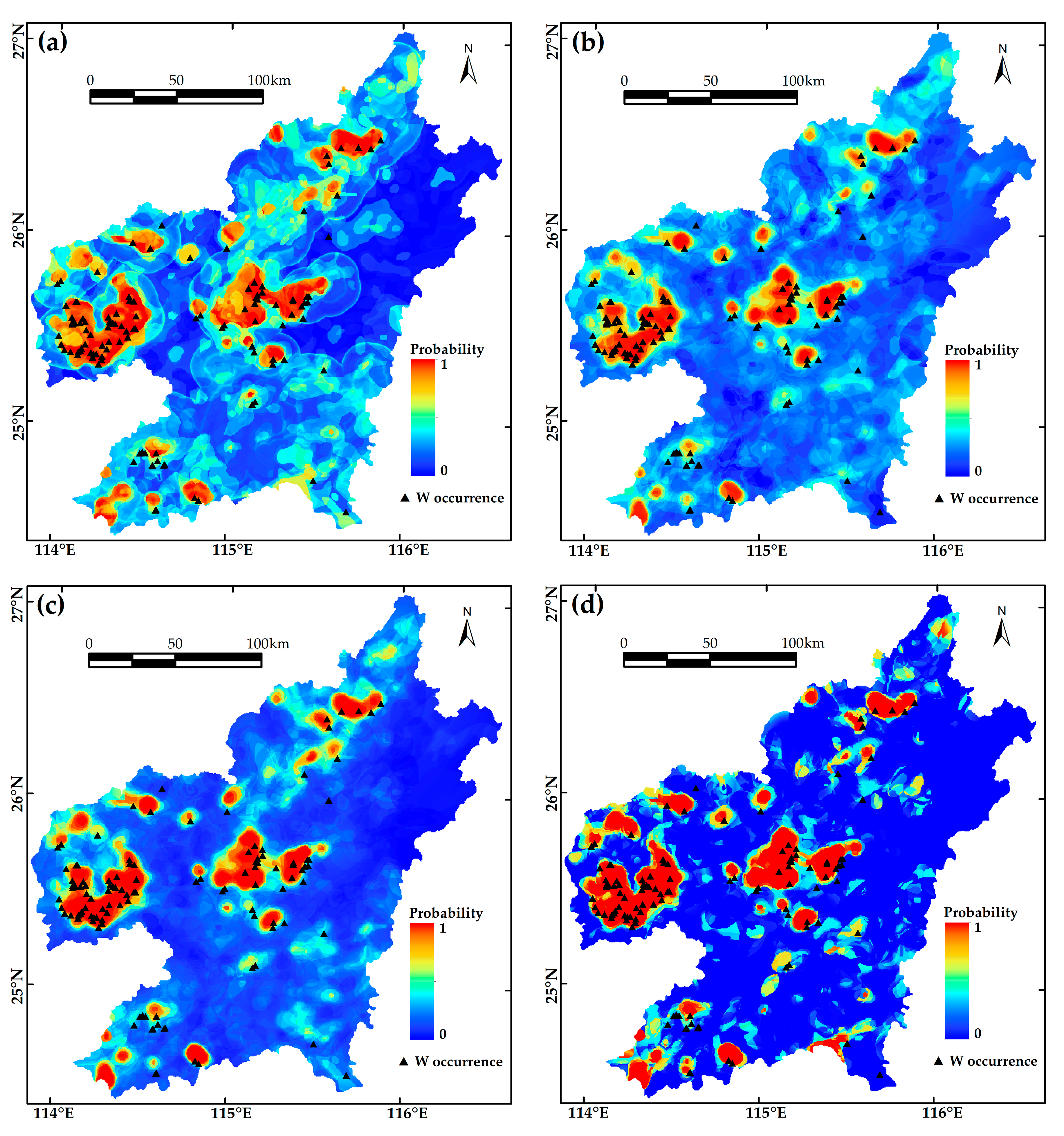
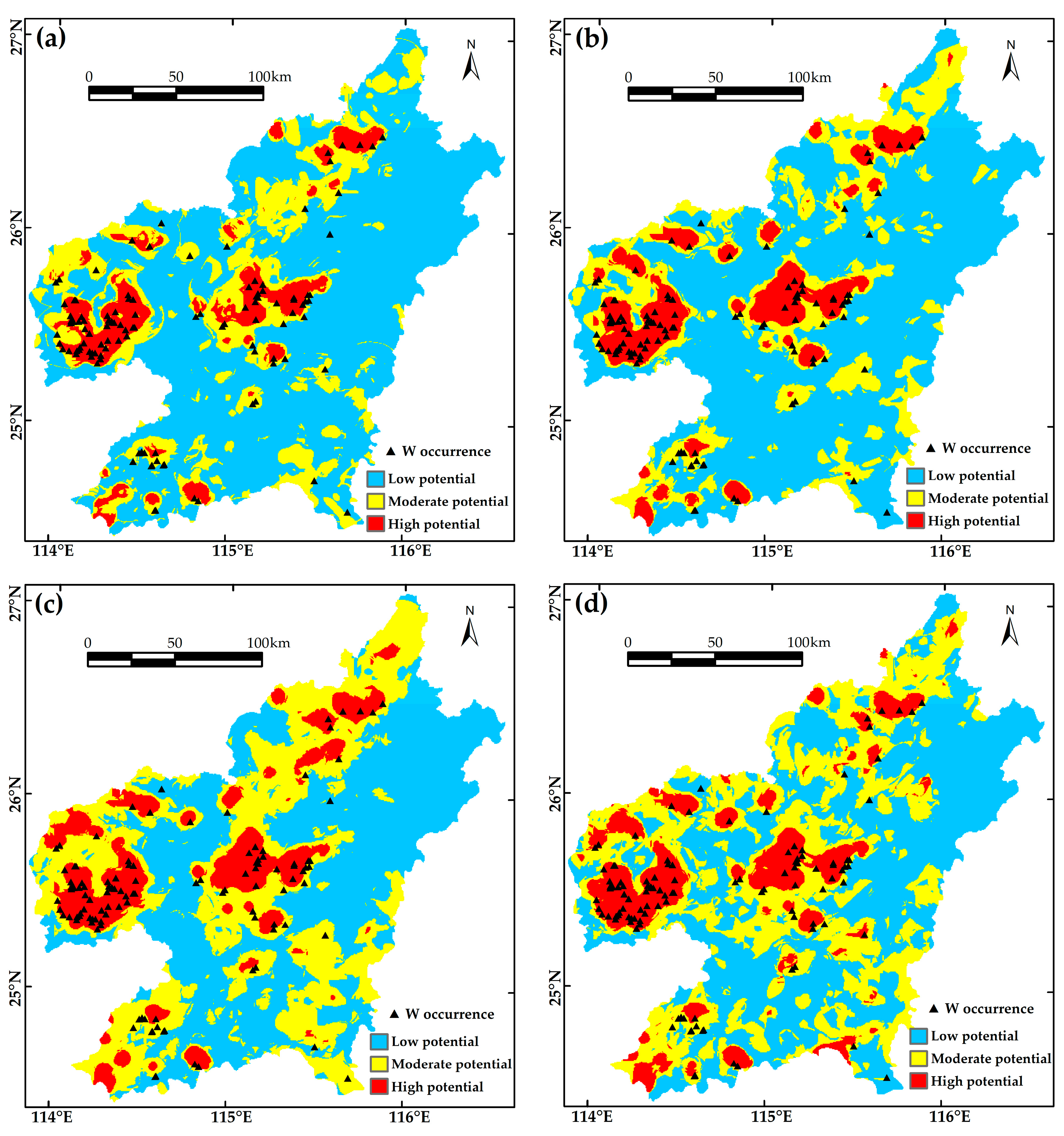
The success-rate curve is straightforward in revealing the predictive efficiency of models. As shown in Figure 12, the success-rate curve of each model can be fit by three regression lines with different slopes. A steeper slope is indicative of higher predictive efficiency. The identified prospective zones capture more known occurrences within smaller delineated areas. In this sense, prospectivity zoning can be conducted based on the thresholds identified by the intersection of the neighboring regression lines that reveal high, moderate and low potential for discovering new W occurrences (Figure 13). It is worth noting that only the zones of high potential, commonly with a success-rate curve slope greater than 5, are prospective areas suitable for further exploration. Other areas have a slope equal to or lower than 1, equivalent to, or lower than the natural distributed density (i.e., every 1% of the area contains 1% of the mineral occurrences). Therefore, the predictive efficiency of ML models depends on the slope of the first segment of the success-rate curve. The RF model achieves the most efficient predictive performance with the highest slope of 6.7797, delineating the high potential areas that cover only 9% of the total area, but capture 66.95% of existing occurrences. The SVM (6.4241), CNN (5.3232), and ANN (5.1835) models perform less efficiently according to their lower slopes. The priority rank of the models revealed by the success-rate curves is consistent ranking based on ROC curves (Figure 12 and Figure 13).

Considering both classification accuracy and predictive capability, it can be concluded that the CNN model is the best recognition engine, but not a good predictor for the MPM application of the study area, whereas the RF model is a good recognition engine and the best predictor. The RF model is selected as the optimal model for exploration targeting since the predictive efficiency should be ranked first in the decision-making process of further mineral exploration. Thus, the predictive map generated by the RF model is utilized as the final prospectivity map (Figure 13a).

In this study, the RF model achieves the most excellent predictive performance. The RF model also outperformed the other models in almost all ML-based MPM studies (e.g., [5,24,27,28,82]). This may be attributed to the random sampling scenarios used in RF training processes providing great diversity derived from limited original data, and thus effectively avoid over-fitting.

5.3. Geological Interpretation of Predictive Models and Implications for Future Mineral Exploration

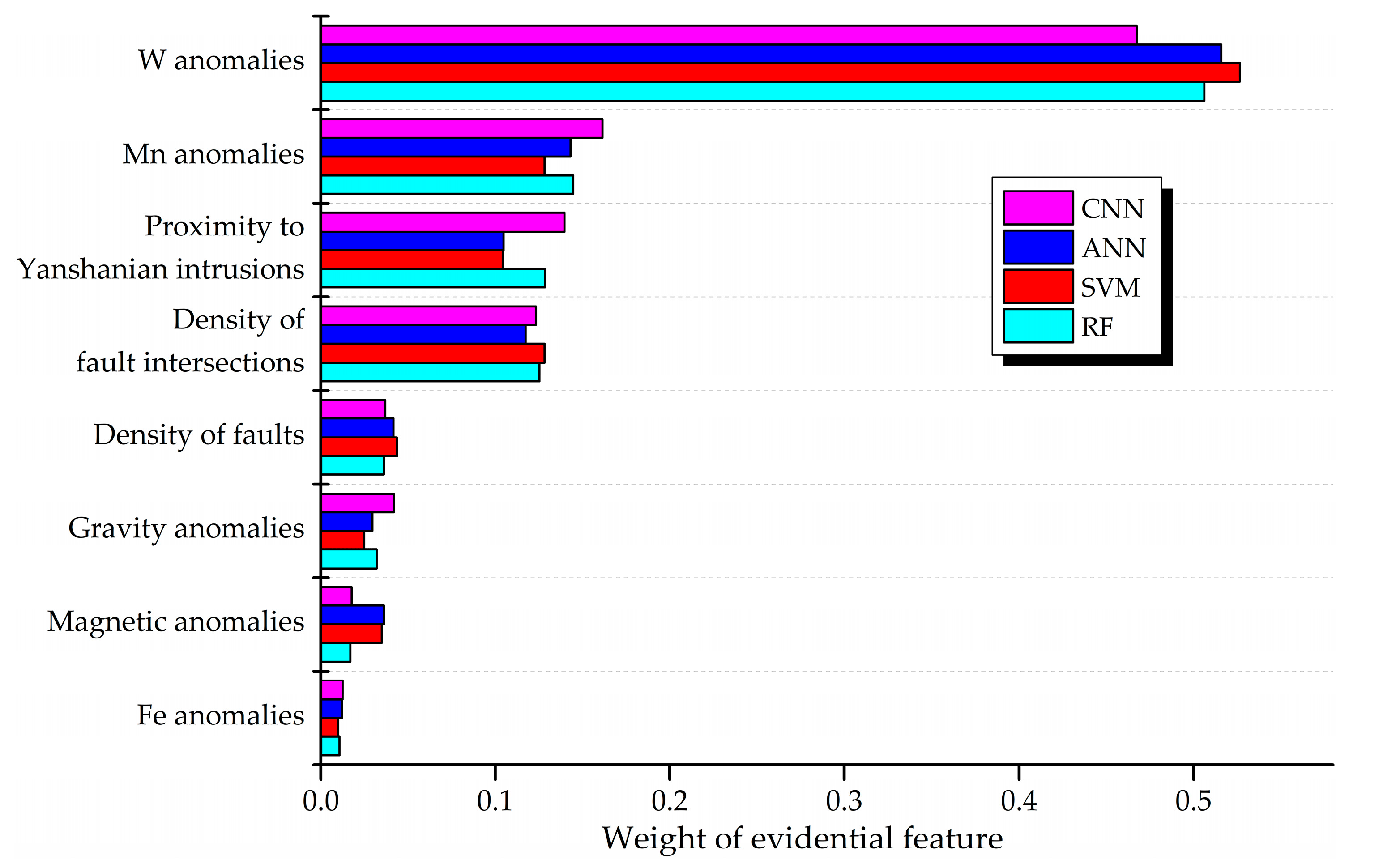
The interpretation of modelling results was conducted by quantifying the relative importance of each evidential feature contributing to the final predictive models (Figure 14). W anomaly makes the most important contribution to the four predictive models, followed by Mn anomaly, proximity to Yanshanian intrusions, and density of fault intersections. Other features do not contribute significantly as predictor variables in the MPM modelling. Among the important predictor variables, W anomaly is the direct indication for the targeted mineralization in the study area, thus exerting the greatest influence on the predictive modelling. It is worth pointing out that Mn anomaly imposes a significant influence on predictive models. Such influence is even greater than the influences exerted by proximity to Yanshanian intrusions and regional structures that are well-recognized ore-controlling factors. Although W, Mn, and Fe are critical components of wolframite that dominates the tungstate of the ores in the study area, and geochemical anomalies have long been emphasized in the practical mineral exploration, Mn and Fe anomalies were previously neglected, because it was assumed all ore-forming elements of wolframite originated from magmatic fluids [83,84,85]. However, a recent study demonstrates that Fe and Mn contributed by host rocks exerts a decisive control on wolframite precipitation in the Panasqueira region (Portugal), and infers that Fe enrichment in the host rocks leads to the predominance of ferberite (FeWO₄) in the wolframite ores [86]. The fluid–rock interaction may also play a crucial role in the formation of wolframite in the southern Jiangxi Province, and Mn/Fe enrichment in the wall rocks may be a prerequisite for wolframite formation. Some evidences are summarized below. (i) In a recent work conducted on the Xihuashan deposit in the study area [46], the LA-ICP-MS analyses of fluid inclusion indicate that mineralized fluid is depleted in Fe and Mn. The occurrences of siderite and pyrophanite in the wall rocks are evidences of Fe and Mn release during wall rock alteration. (ii) In an unpublished work conducted by Wu (one of the co-authors of this paper), intensive alteration was observed in the wall rocks adjacent to wolframite-bearing ore veins in the Piaotang deposit in the study area. Chlorite and biotite were replaced by muscovite and pyrophanite. The pyrophanite and residual chlorite widely distributed in the wall rocks formed a zone enriched in Mn/Fe. The proximal wall rocks can provide sufficient Mn/Fe source for wolframite precipitation when W-enriched fluids encountered these rocks. The metal source of Mn/Fe from the wall rocks can explain why Mn anomalies exert a significant influence on W prospectivity modelling in this study. The spatial correlation of Mn anomalies and W mineralization in the study area is also revealed by a weights-of-evidence analysis [65]. It is also noted that Fe anomaly provides little evidential information for predicting W mineralization, which may be ascribed to (i) majority of hubnerite (MnWO₄) in the wolframite ores from W-Sn deposits that dominate the W-polymetallic mineralization in the study area [87], and (ii) interference from widely distributed Fe-enriched Cretaceous red beds formed after W mineralization in the study area. Ore-forming materials of wall rocks played an important role in the formation of wolframite ores, and the Mn anomaly should be regarded as an important exploration criterion. This criterion may facilitate the future tungsten prospecting and provide insights into the genetic model of tungsten mineralization in this area.

6. Conclusions and Future Work

Predictive modelling of mineral prospectivity was carried out in the southern Jiangxi Province. Based on abundant exploration data and publicly accessible multi-source geo-information, three input datasets including 118 known occurrences, 118 randomly selected non-occurrences, and eight evidential features related to W mineralization were prepared. A set of ML models including RF, SVM, and ANN, as well as the deep learning CNN model were trained by using different input datasets, and the performances of the resulting models were assessed by the confusion matrix, ROC curve, and success-rate curve.

In the training process, CNN and RF models present great accuracy and stability against variations of model parameters. The sensitivity analysis reveals that elaborate models with complex architecture do not necessarily improve predictive performance in the MPM of the study area. Predictive performance of trained models was comprehensively assessed and compared in order to select the optimal one to generate the prospectivity map. With respect to classification accuracy, the CNN model achieves the most accurate performance that correctly classifies 92.38% of labelled samples, and leads to other statistical indices derived from confusion matrices, followed by RF, SVM, and ANN models. The overall predictive performance of ML models was evaluated by the ROC curves, which reveals that the RF model outperforms the rest of ML models. The success-rate curves indicate that the prospective zones identified by the RF model capture more known W occurrences in smaller delineated areas, suggesting the most efficient predictive performance. Regarding the above measurements of model assessment, the RF model was chosen as the best model to generate the prospectivity model for further exploration in the study area. The high potential areas capture 66.95% existing occurrences within 9% of the total area of this region. The modelling results rank the relative importance of evidential features contributing to the predictions. It is revealed that W anomalies, Mn anomalies, proximity to Yanshanian intrusions, and density of fault intersections are the most significant features for predicting W mineralization. Mn anomalies in the host rocks represent an innovative exploration criterion that has been long neglected in the practical mineral exploration in the study area, and can provide insights into the genetic model of W mineralization in this region.

There are some limitations in the MPM of this study, and further work needs to be carried out in the future. Firstly, although the spatial and genetic associations of Mn anomalies and W mineralization have been demonstrated in this study, it is worth noting that Mn is coprecipitated in steam sediments and is sensitive to oxidation–reduction reaction in the water. More reliable data, such as rock and soil geochemical data, should be collected and analyzed when applying the prospectivity model and targeting Mn anomalies as an indicator of W mineralization in the future prospecting work. Secondly, the applicability of ML models can be enhanced. There are two main factors that undermine the advantageous performances of artificial intelligence models in MPM field: (i) The mineral occurrences used for training ML models are scarce when compared to thousands of samples employed in the image recognition field, and (ii) the mineralization pattern under recognition are too complex to be efficiently captured by limited training data, because mineralization is an end-product of complex interplays of ore-forming processes that leave behind its signatures of patterns in the form of various nonlinear-correlated geological features. In this regard, more efforts, including imbed of knowledge-driven engine and use of effectively lucid expression of evidential layers, have to be made to “help” ML models learn the complex mineral systems in future work, given that the problem of scarce input data cannot be solved at this stage.

References

- Carranza, E.J.M.; Laborte, A.G. Data-driven predictive mapping of gold prospectivity, Baguio district, Philippines: Application of random forests algorithm. Ore. Geol. Rev. 2015, 71, 777–787. [Google Scholar] [CrossRef]
- Yousefi, M.; Carranza, E.J.M. Geometric average of spatial evidence data layers: A GIS-based multi-criteria decision-making approach to mineral prospectivity mapping. Comput. Geosci. 2015, 83, 72–79. [Google Scholar] [CrossRef]
- Porwal, A.; Carranza, E.J.M. Introduction to the special issue: GIS-based mineral potential modelling and geological data analyses for mineral exploration. Ore. Geol. Rev. 2015, 71, 477–483. [Google Scholar] [CrossRef]
- Yousefi, M.; Nykänen, V. Introduction to the special issue: GIS-based mineral potential targeting. J. Afr. Earth. Sci. 2017, 128, 1–4. [Google Scholar] [CrossRef]
- Rodriguez-Galiano, V.; Sanchez-Castillo, M.; Chica-Olmo, M.; Chica-Rivas, M. Machine learning predictive models for mineral prospectivity: An evaluation of neural networks, random forest, regression trees and support vector machines. Ore. Geol. Rev. 2015, 71, 804–818. [Google Scholar] [CrossRef]
- Carranza, E.J.M. Geocomputation of mineral exploration targets. Comput. Geosci. 2011, 37, 1907–1916. [Google Scholar] [CrossRef]
- Cheng, Q.; Agterberg, F.P. Fuzzy weights of evidence method and its application in mineral potential mapping. Nat. Resour. Res. 1999, 8, 27–35. [Google Scholar] [CrossRef]
- Zuo, R.; Cheng, Q.; Agterberg, F.P. Application of a hybrid method combining multilevel fuzzy comprehensive evaluation with asymmetric fuzzy relation analysis to mapping prospectivity. Ore. Geol. Rev. 2009, 35, 101–108. [Google Scholar] [CrossRef]
- Yousefi, M.; Nykänen, V. Data-driven logistic-based weighting of geochemical and geological evidence layers in mineral prospectivity mapping. J. Geochem. Explor. 2016, 164, 94–106. [Google Scholar] [CrossRef]
- Li, B.; Liu, B.; Guo, K.; Li, C.; Wang, B. Application of a maximum entropy model for mineral prospectivity maps. Minerals 2019, 9, 556. [Google Scholar] [CrossRef] [Green Version]
- Li, X.; Yuan, F.; Zhang, M.; Jia, C.; Jowitt, S.M.; Ord, A.; Zheng, T.; Hu, X.; Li, Y. Three-dimensional mineral prospectivity modeling for targeting of concealed mineralization within the Zhonggu iron orefield, Ningwu basin, China. Ore. Geol. Rev. 2015, 71, 633–654. [Google Scholar] [CrossRef]
- Leite, E.P.; de Souza Filho, C.R. Probabilistic neural networks applied to mineral potential mapping for platinum group elements in the Serra Leste region, Carajás Mineral Province, Brazil. Comput. Geosci. 2009, 35, 675–687. [Google Scholar] [CrossRef]
- Porwal, A.; Carranza, E.J.M.; Hale, M. Bayesian network classifiers for mineral potential mapping. Comput. Geosci. 2006, 32, 1–16. [Google Scholar] [CrossRef]
- Singer, D.A.; Kouda, R. Classification of mineral deposits into types using mineralogy with a probabilistic neural network. Nonrenew. Resour. 1997, 6, 27–32. [Google Scholar] [CrossRef]
- Carranza, E.J.M.; Hale, M. Logistic regression for geologically constrained mapping of gold potential, Baguio district, Philippines. Explor. Min. Geol. 2001, 10, 165–175. [Google Scholar] [CrossRef]
- Li, X.; Yuan, F.; Zhang, M.; Jowitt, S.M.; Ord, A.; Zhou, T.; Dai, W. 3D computational simulation-based mineral prospectivity modeling for exploration for concealed Fe–Cu skarn-type mineralization within the Yueshan orefield, Anqing district, Anhui province, China. Ore. Geol. Rev. 2019, 105, 1–17. [Google Scholar] [CrossRef]
- Qin, Y.; Liu, L. Quantitative 3D association of geological factors and geophysical fields with mineralization and its significance for ore prediction: An example from Anqing orefield, China. Minerals 2018, 8, 300. [Google Scholar] [CrossRef] [Green Version]
- Zuo, R. Machine learning of mineralization-related geochemical anomalies: A review of potential methods. Nat. Resour. Res. 2017, 26, 457–464. [Google Scholar] [CrossRef]
- Lary, D.J.; Alavi, A.H.; Gandomi, A.H.; Walker, A.L. Machine learning in geosciences and remote sensing. Geosci. Front. 2016, 7, 3–10. [Google Scholar] [CrossRef] [Green Version]
- Wegner, J.; Roscher, R.; Volpi, M.; Veronesi, F. Foreword to the special issue on machine learning for geospatial data analysis. Isprs. Int. J. Geo-Inf. 2018, 7, 147. [Google Scholar]
- Lee, J.; Jang, H.; Yang, J.; Yu, K. Machine learning classification of buildings for map generalization. Isprs. Int. J. Geo-Inf. 2017, 6, 309. [Google Scholar] [CrossRef] [Green Version]
- Saljoughi, B.S.; Hezarkhani, A. A comparative analysis of artificial neural network (ANN), wavelet neural network (WNN), and support vector machine (SVM) data-driven models to mineral potential mapping for copper mineralizations in the Shahr-e-Babak region, Kerman, Iran. Appl. Geomat. 2018, 10, 229–256. [Google Scholar] [CrossRef]
- Chen, Y.; Wu, W.; Zhao, Q. A bat-optimized one-class support vector machine for mineral prospectivity mapping. Minerals 2019, 9, 317. [Google Scholar] [CrossRef] [Green Version]
- Sun, T.; Chen, F.; Zhong, L.; Liu, W.; Wang, Y. Gis-based mineral prospectivity mapping using machine learning methods: A case study from Tongling ore district, eastern China. Ore. Geol. Rev. 2019, 109, 26–49. [Google Scholar] [CrossRef]
- Li, T.; Xia, Q.; Zhao, M.; Gui, Z.; Leng, S. Prospectivity mapping for tungsten polymetallic mineral resources, Nanling metallogenic belt, south China: Use of random forest algorithm from a perspective of data imbalance. Nat. Resour. Res. 2019. [Google Scholar] [CrossRef]
- Zhang, N.; Zhou, K.; Li, D. Back-propagation neural network and support vector machines for gold mineral prospectivity mapping in the Hatu region, Xinjiang, China. Earth. Sci. Inform. 2018, 11, 553–566. [Google Scholar] [CrossRef]
- Zhang, Z.; Zuo, R.; Xiong, Y. A comparative study of fuzzy weights of evidence and random forests for mapping mineral prospectivity for skarn-type fe deposits in the southwestern Fujian metallogenic belt, China. Sci. China. Earth. Sci. 2015, 59, 556–572. [Google Scholar] [CrossRef]
- Carranza, E.J.M.; Laborte, A.G. Random forest predictive modeling of mineral prospectivity with small number of prospects and data with missing values in Abra (Philippines). Comput. Geosci. 2015, 74, 60–70. [Google Scholar] [CrossRef]
- LeCun, Y.; Bengio, Y.; Hinton, G. Deep learning. Nature 2015, 521, 436–444. [Google Scholar] [CrossRef]
- Young, T.; Hazarika, D.; Poria, S.; Cambria, E. Recent trends in deep learning based natural language processing. IEEE Comput. Intell. M. 2018, 13, 55–75. [Google Scholar] [CrossRef]
- Dekhtiar, J.; Durupt, A.; Bricogne, M.; Eynard, B.; Rowson, H.; Kiritsis, D. Deep learning for big data applications in CAD and PLM–Research review, opportunities and case study. Comput. Ind. 2018, 100, 227–243. [Google Scholar] [CrossRef]
- Wang, Y.; Fang, Z.; Hong, H. Comparison of convolutional neural networks for landslide susceptibility mapping in Yanshan County, China. Sci. Total. Environ. 2019, 666, 975–993. [Google Scholar] [CrossRef] [PubMed]
- Xiao, L.; Zhang, Y.; Peng, G. Landslide susceptibility assessment using integrated deep learning algorithm along the China-Nepal highway. Sensors 2018, 18, 4436. [Google Scholar] [CrossRef] [PubMed] [Green Version]
- Zuo, R.; Xiong, Y.; Wang, J.; Carranza, E.J.M. Deep learning and its application in geochemical mapping. Earth-Sci. Rev. 2019, 192, 1–14. [Google Scholar] [CrossRef]
- Miller, J.; Nair, U.; Ramachandran, R.; Maskey, M. Detection of transverse cirrus bands in satellite imagery using deep learning. Comput. Geosci. 2018, 118, 79–85. [Google Scholar] [CrossRef]
- Xiong, Y.; Zuo, R.; Carranza, E.J.M. Mapping mineral prospectivity through big data analytics and a deep learning algorithm. Ore. Geol. Rev. 2018, 102, 811–817. [Google Scholar] [CrossRef]
- Carranza, E.J.M.; van Ruitenbeek, F.J.A.; Hecker, C.; van der Meijde, M.; van der Meer, F.D. Knowledge-guided data-driven evidential belief modeling of mineral prospectivity in Cabo de Gata, SE Spain. Int. J. Appl. Earth. Obs. 2008, 10, 374–387. [Google Scholar] [CrossRef]
- Feng, C.; Zhang, D.; Zeng, Z.; Wang, S. Chronology of the tungsten deposits in southern Jiangxi Province, and episodes and zonation of the regional W-Sn mineralization-evidence from high-precision zircon U-Pb, molybdenite Re-Os and muscovite Ar-Ar ages. Acta. Geol. Sin-Engl. 2012, 86, 555–567. [Google Scholar]
- Feng, C.; Zeng, Z.; Zhang, D.; Qu, W.; Du, A.; Li, D.; She, H. Shrimp zircon U–Pb and molybdenite Re–Os isotopic dating of the tungsten deposits in the Tianmenshan–Hongtaoling W–Sn orefield, southern Jiangxi Province, China, and geological implications. Ore. Geol. Rev. 2011, 43, 8–25. [Google Scholar] [CrossRef]
- Jingwen, M.; Yanbo, C.; Maohong, C.; Pirajno, F. Major types and time–space distribution of Mesozoic ore deposits in south China and their geodynamic settings. Miner. Depos. 2013, 48, 267–294. [Google Scholar] [CrossRef]
- Mao, J.; Xie, G.; Guo, C.; Chen, Y. Large-scale tungsten-tin mineralization in the Nanling Region, south China: Metallogenic ages and corresponding geodynamic processes. Acta Petrol. Sin. 2007, 23, 2329–2338. [Google Scholar]
- Zhao, W.W.; Zhou, M.F.; Li, Y.H.M.; Zhao, Z.; Gao, J.F. Genetic types, mineralization styles, and geodynamic settings of Mesozoic tungsten deposits in south China. J. Asian. Earth. Sci. 2017, 137, 109–140. [Google Scholar] [CrossRef]
- Liang, X.; Dong, C.; Jiang, Y.; Wu, S.; Zhou, Y.; Zhu, H.; Fu, J.; Wang, C.; Shan, Y. Zircon U–Pb, molybdenite Re–Os and muscovite Ar–Ar isotopic dating of the Xitian W–Sn polymetallic deposit, eastern Hunan Province, south China and its geological significance. Ore. Geol. Rev. 2016, 78, 85–100. [Google Scholar] [CrossRef]
- Yang, J.H.; Kang, L.F.; Peng, J.T.; Zhong, H.; Gao, J.F.; Liu, L. In-situ elemental and isotopic compositions of apatite and zircon from the Shuikoushan and Xihuashan granitic plutons: Implication for Jurassic granitoid-related Cu-Pb-Zn and W mineralization in the Nanling Range, south China. Ore. Geol. Rev. 2018, 93, 382–403. [Google Scholar] [CrossRef]
- Yang, J.H.; Kang, L.F.; Liu, L.; Peng, J.T.; Qi, Y.Q. Tracing the origin of ore-forming fluids in the Piaotang tungsten deposit, south China: Constraints from in-situ analyses of wolframite and individual fluid inclusion. Ore. Geol. Rev. 2019, 111, 102939. [Google Scholar] [CrossRef]
- Yang, J.H.; Zhang, Z.; Peng, J.T.; Liu, L.; Leng, C.B. Metal source and wolframite precipitation process at the Xihuashan tungsten deposit, south China: Insights from mineralogy, fluid inclusion and stable isotope. Ore. Geol. Rev. 2019, 111, 102965. [Google Scholar] [CrossRef]
- Nanling Range Group of Ministry of Geology and Mineral Resources. Study on Regional Tectonic Characteristics and Ore-Forming Structures in the Nanling Range; Geology Publishing House: Beijing, China, 1988; p. 266. (In Chinese) [Google Scholar]
- Fang, G.; Chen, Z.; Chen, Y.; Li, J.; Zhao, B.; Zhou, X.; Zeng, Z.; Zhang, Y. Geophysical investigations of the geology and structure of the Pangushan-Tieshanlong tungsten ore field, South Jiangxi, China—Evidence for site-selection of the 2000-m nanling scientific drilling project (SP-NLSD-2). J. Asian. Earth. Sci. 2015, 110, 10–18. [Google Scholar] [CrossRef]
- GeoCloud Database of China Geological Survey. Available online: http://geocloud.cgs.gov.cn (accessed on 31 December 2019).
- Breiman, L. Random forests. Mach. Learn. 2001, 45, 5–32. [Google Scholar] [CrossRef] [Green Version]
- Rodriguez-Galiano, V.F.; Chica-Olmo, M.; Chica-Rivas, M. Predictive modelling of gold potential with the integration of multisource information based on random forest: A case study on the Rodalquilar area, Southern Spain. Int. J. Geogr. Inf. Sci. 2014, 28, 1336–1354. [Google Scholar] [CrossRef]
- Breiman, L.; Friedman, J.; Stone, C.J.; Olshen, R.A. Classification and Regression Trees; Chapman and Hall/CRC: London, UK, 1984; p. 368. [Google Scholar]
- Vapnik, V. The Nature of Statistical Learning Theory; Springer-Verlag: New York, NY, USA, 2000; p. 314. [Google Scholar]
- Asadi, H.H.; Hale, M. A predictive GIS model for mapping potential gold and base metal mineralization in Takab area, Iran. Comput. Geosci. 2001, 27, 901–912. [Google Scholar] [CrossRef]
- Mahvash Mohammadi, N.; Hezarkhani, A. Application of support vector machine for the separation of mineralised zones in the Takht-e-Gonbad porphyry deposit, SE Iran. J. Afr. Earth. Sci. 2018, 143, 301–308. [Google Scholar] [CrossRef]
- Huang, C.; Davis, L.S.; Townshend, J.R.G. An assessment of support vector machines for land cover classification. Int. J. Remote. Sens. 2002, 23, 725–749. [Google Scholar] [CrossRef]
- Burges, C.J.C. A tutorial on support vector machines for pattern recognition. Data. Min. Knowl. Disc. 1998, 2, 121–167. [Google Scholar] [CrossRef]
- Zuo, R.; Carranza, E.J.M. Support vector machine: A tool for mapping mineral prospectivity. Comput. Geosci. 2011, 37, 1967–1975. [Google Scholar] [CrossRef]
- Zaremotlagh, S.; Hezarkhani, A. The use of decision tree induction and artificial neural networks for recognizing the geochemical distribution patterns of LREE in the Choghart deposit, Central Iran. J. Afr. Earth. Sci. 2017, 128, 37–46. [Google Scholar] [CrossRef]
- Celik, U.; Basarir, C. The prediction of precious metal prices via artificial neural network by using RapidMiner. Alphan. J. 2017, 5, 45. [Google Scholar] [CrossRef]
- Brown, W.M.; Gedeon, T.D.; Groves, D.I.; Barnes, R.G. Artificial neural networks: A new method for mineral prospectivity mapping. Aust. J. Earth. Sci. 2000, 47, 757–770. [Google Scholar] [CrossRef]
- Panda, L.; Tripathy, S.K. Performance prediction of gravity concentrator by using artificial neural network-a case study. Int. J. Min. Sci. Technol. 2014, 24, 461–465. [Google Scholar] [CrossRef]
- Imamverdiyev, Y.; Sukhostat, L. Lithological facies classification using deep convolutional neural network. J. Petrol. Sci. Eng. 2019, 174, 216–228. [Google Scholar] [CrossRef]
- Ghorbanzadeh, O.; Blaschke, T.; Gholamnia, K.; Meena, S.; Tiede, D.; Aryal, J. Evaluation of different machine learning methods and deep-learning convolutional neural networks for landslide detection. Remote. Sens. 2019, 11, 196. [Google Scholar] [CrossRef] [Green Version]
- Sun, T.; Wu, K.; Chen, L.; Liu, W.; Wang, Y.; Zhang, C. Joint application of fractal analysis and weights-of-evidence method for revealing the geological controls on regional-scale tungsten mineralization in southern Jiangxi Province, China. Minerals 2017, 7, 243. [Google Scholar] [CrossRef] [Green Version]
- Jiangxi Bureau of Geology and Mineral Resources. Mineral Prospecting and Targeting of W-Sn-Pb-Zn Deposits in Southern Jiangxi Province; Jiangxi Bureau of Geology and Mineral Resources: Nanchang, China, 2002; p. 112. (In Chinese) [Google Scholar]
- Chen, X.; Fu, J. Geochemical Maps of Nanling Range; China University of Geoscience Press: Wuhan, China, 2012; p. 109. (In Chinese) [Google Scholar]
- Xie, X.J.; Mu, X.Z.; Ren, T.X. Geochemical mapping in China. J. Geochem. Explor. 1997, 60, 99–113. [Google Scholar]
- Xie, X.J.; Ren, T.X.; Xi, X.H.; Zhang, L.S. The Implementation of the regional geochemistry-National Reconnaissance Program (RGNR) in China in the past thirty years. Acta Geosci. Sin. 2009, 30, 700–716. (In Chinese) [Google Scholar]
- Carranza, E.J.M. Objective selection of suitable unit cell size in data-driven modeling of mineral prospectivity. Comput. Geosci. 2009, 35, 2032–2046. [Google Scholar] [CrossRef]
- Hengl, T. Finding the right pixel size. Comput. Geosci. 2006, 32, 1283–1298. [Google Scholar] [CrossRef]
- Carranza, E.J.M.; Hale, M.; Faassen, C. Selection of coherent deposit-type locations and their application in data-driven mineral prospectivity mapping. Ore. Geol. Rev. 2008, 33, 536–558. [Google Scholar] [CrossRef]
- Badel, M.; Angorani, S.; Shariat Panahi, M. The application of median indicator Kriging and neural network in modeling mixed population in an iron ore deposit. Comput. Geosci. 2011, 37, 530–540. [Google Scholar] [CrossRef]
- Porwal, A.; Carranza, E.J.M.; Hale, M. Artificial neural networks for mineral-potential mapping: A case study from Aravalli Province, western India. Nat. Resour. Res. 2003, 12, 155–171. [Google Scholar] [CrossRef]
- Xiong, Y.; Zuo, R. Effects of misclassification costs on mapping mineral prospectivity. Ore. Geol. Rev. 2017, 82, 1–9. [Google Scholar] [CrossRef]
- Liu, C.; Berry, P.M.; Dawson, T.P.; Pearson, R.G. Selecting thresholds of occurrence in the prediction of species distributions. Ecography 2005, 28, 385–393. [Google Scholar] [CrossRef]
- Tien Bui, D.; Tuan, T.A.; Klempe, H.; Pradhan, B.; Revhaug, I. Spatial prediction models for shallow landslide hazards: A comparative assessment of the efficacy of support vector machines, artificial neural networks, kernel logistic regression, and logistic model tree. Landslides 2015, 13, 361–378. [Google Scholar] [CrossRef]
- Nykänen, V.; Lahti, I.; Niiranen, T.; Korhonen, K. Receiver operating characteristics (ROC) as validation tool for prospectivity models—A magmatic Ni–Cu case study from the Central Lapland Greenstone Belt, Northern Finland. Ore. Geol. Rev. 2015, 71, 853–860. [Google Scholar] [CrossRef]
- Nykänen, V.; Niiranen, T.; Molnár, F.; Lahti, I.; Korhonen, K.; Cook, N.; Skyttä, P. Optimizing a knowledge-driven prospectivity model for gold deposits within Peräpohja Belt, Northern Finland. Nat. Resour. Res. 2017, 26, 571–584. [Google Scholar] [CrossRef]
- Tien Bui, D.; Ho, T.-C.; Pradhan, B.; Pham, B.-T.; Nhu, V.-H.; Revhaug, I. GIS-based modeling of rainfall-induced landslides using data mining-based functional trees classifier with adaboost, bagging, and multiboost ensemble frameworks. Environ. Earth Sci. 2016, 75, 1101. [Google Scholar] [CrossRef]
- Murphy, K.P. Machine Learning: A Probabilistic Perspective; The MIT Press: Londong, UK, 2012; p. 1096. [Google Scholar]
- McKay, G.; Harris, J.R. Comparison of the data-driven random forests model and a knowledge-driven method for mineral prospectivity mapping: A case study for gold deposits around the Huritz Group and Nueltin Suite, Nunavut, Canada. Nat. Resour. Res. 2015, 25, 125–143. [Google Scholar] [CrossRef]
- Group of Tungsten Deposits in Nanling Range of Ministry of Metallurgy. Tungsten Deposits in South China; Metallurgical Industry Press: Beijing, China, 1985; p. 496. (In Chinese) [Google Scholar]
- Fang, G.C.; Tong, Q.Q.; Sun, J.; Zhu, G.H.; Chen, Z.H.; Zeng, Z.L.; Liu, K.L. Stable isotope geochemical characteristics of Pangushan tungsten deposit in southern Jiangxi Province. Miner. Depo. 2014, 33, 1391–1399. (In Chinese) [Google Scholar]
- Xu, T.; Wang, Y. Sulfur and lead isotope composition on tracing ore-forming materials of the Xihuashan tungsten deposit in southern Jiangxi. Bull. Miner. Petrol. Geochem. 2014, 33, 342–347. (In Chinese) [Google Scholar]
- Lecumberri-Sanchez, P.; Vieira, R.; Heinrich, C.A.; Pinto, F.; Wӓlle, M. Fluid-rock interaction is decisive for the formation of tungsten deposits. Geology 2017, 45, 579–582. [Google Scholar] [CrossRef]
- Tan, Y.J. Composition characteristics and controlling factors of tungsten mineral of the endogenetic tungsten deposits in South China. China Tungsten Ind. 1999, 14, 84–89. (In Chinese) [Google Scholar]
Figure 1.
Simplified geological map of the study area, modified from [
39,
48,
49].
Figure 2.
Sketch showing positions of different types of W mineralization relative to Yanshanian intrusions, modified from [
42].
Figure 3.
Examples illustrating the operations of convolution (a) and max pooling (b).
Figure 4.
Typical architecture of one-dimensional CNNmodel.
Figure 5.
Evidential features used as predictor variables for prospectivity modelling: (a) Proximity to Yanshanian intrusions; (b) density of NE-EW trending faults; (c) density of intersections of NE-EW trending faults; (d) gravity anomaly; (e) magnetic anomaly; (f) W anomaly; (g) Fe anomaly; and (h) Mn anomaly.
Figure 6.
Plot of distances and corresponding probabilities that one W occurrence is situated next to another known W occurrence.
Figure 7.
Locations of known mineral occurrences and selected non-occurrences.
Figure 8.
Results of sensitivity analyses showing the classification errors (MSE) for possible combinations of parameters for training each machine learning model: Number of trees and number of features used for training RF models based on Dataset 1 (a), Dataset 2 (b), and Dataset 3 (c); gamma and cost used for training SVM models based on Dataset 1 (d), Dataset 2 (e), and Dataset 3 (f); number of neurons and learning rate used for training ANN models based on Dataset 1 (g), Dataset 2 (h), and Dataset 3 (i); number of feature maps and number of neurons used for training CNN models based on Dataset 1 (j), Dataset 2 (k), and Dataset 3 (l).
Figure 9.
Box plot showing the statistical results of MSE against the variations of parameters related to model complexity: (a) number of trees employed in RF; (b) number of neurons employed in ANN; (c) number of feature maps employed in CNN; and (d) number of neurons employed in CNN.
Figure 10.
Predictive maps showing average probability output by machine learning models based on three input datasets: (a) RF; (b) SVM; (c) ANN; and (d) CNN models.
Figure 11.
ROC curves and AUCs of ML models trained by Dataset 1 (a), Dataset 2 (b), and Dataset 3 (c).
Figure 12.
Success-rate curves of predictive models: (a) RF; (b) SVM; (c) ANN; and (d) CNN models.
Figure 13.
Prospectivity maps of (
a) RF, (
b) SVM, (
c) ANN, and (
d) CNN models showing different potential areas delineated by the thresholds identified from
Figure 14.
Weights obtained by information gain indicating the contribution of each evidential feature to predictions.