Novel Approach to Modeling the Seismic Waves in the Areas with Complex Fractured Geological Structures


Applied Computational Geophysics Lab, Moscow Institute of Physics and Technology, 141701 Dolgoprudny, Russia
*
Author to whom correspondence should be addressed.
Minerals 2020, 10(2), 122; https://0-doi-org.brum.beds.ac.uk/10.3390/min10020122
Submission received: 18 November 2019
/
Revised: 24 January 2020
/
Accepted: 28 January 2020
/
Published: 30 January 2020
(This article belongs to the Special Issue Geophysics for Mineral Exploration)
Abstract
:This paper presents a novel approach to modeling the propagation of seismic waves in a medium containing subvertical fractured inhomogeneities, typical for mineralization zones. The developed method allows us to perform calculations on a structural computational grid, which avoids the construction of unstructured grids. For the calculations, the grid-characteristic method is used. We also present a comparison of the proposed method with the one described at earlier works and discuss the areas of its practical application. As an example, the numerical results for a cluster of subvertical fractures are given. A new approach for modeling fractures makes it quite easy to incorporate fractured objects into the seismic models and perform calculations without using algorithms on unstructured and curved grids.
1. Introduction
Many mineral deposits are associated with fractures filled by fluids occurring in volcanic rocks. The seismic method can be effectively used for detection of the fractured zones. Interpretation of seismic data collected over a mineral deposit associated with the fracture fillings requires developing effective methods of modeling the seismic waves in places with micro- and macrocracks. This is one of the challenging areas of mathematical modeling in seismic exploration for mineral deposits. Fault zones and fractures are found in many ore deposits and are important targets in the inversion and interpretation of seismic data. In addition, faults and fractures can have a large impact on the inversion and migration of seismic data (for example, anisotropy caused by fracturing). A variety of fractured structures can also be developed within hydrocarbon deposits in rock formations. They basically form a system of subvertical equally oriented fractures. In order to construct an accurate model of a deposit and develop optimal methods of its exploitation, a good general model of surrounding materials should be created, which requires an accurate reconstruction of the properties and positions of fractures [1].
Over the past few decades, several studies have been conducted on this topic. In 1980, Schoenberg [2] proposed a linear slip model, in which he described a sliding surface with special boundary conditions using approaches based on averaged medium methods. An experimental verification of this model was made in [3]. Numerical simulation of wave propagation a is well-studied area in general, with many approaches proposed to date, such as the most popular finite-difference time-marching schemes [4,5], the spectral elements [6,7], discontinuous Galerkin [8], Helmholtz finite-difference [9,10] or integral-equation solvers [11,12], etc. Still, the development of the numerical methods for modeling the fractured heterogeneities is an area of active research. For example, in [13] the authors investigated the problem of modeling fractures and faults using the finite difference schemes (FDTD). However, this approach allows us to describe and model only those fractured structures which consist of parallel fractures directed along the axes of coordinates (vertical or horizontal). This drawback can be overcome by using non-structural grids for modeling the fractured media. Examples of such approaches can be found in [5,6,7] where the finite-volume methods [14,15] and a grid-characteristic method [16] are used. Unstructured meshes are suitable for calculating the wave propagation in a physical region of complex shape, but they require large additional memory for storing information about the relationships of the mesh’s cells. Recently, the discontinuous Galerkin (DG) method has also been widely used to solve the problems of modeling the propagation of seismic waves. For example, in [17,18], it is used to model the wave fields in the fractured media using an explicit fracture model. The method is also built on unstructured meshes. In [19], three methods were compared: The discontinuous Galerkin method [20,21], the grid-characteristic method on unstructured meshes [16], and the grid-characteristic method on structural grids [22,23,24]. In the work [19], it is shown that the method based on the structural grids has better performance in comparison to the unstructured meshes, in addition to a simpler implementation and operation with the grids. In the work, an anticlinar trap was used as a geological model with a large number of contact surfaces, which is a typical hydrocarbon deposit. Due to the trap structure, the seismogram involves multiple waves, which have to be separated from the useful signal, a task that can hardly be performed with low-order numerical schemes. It is shown, that three numerical methods and their software implementations are suitable for field data computations. Grid-characteristic method on structured grids is much more efficient, since it requires fewer operations per one degree of freedom and has a more efficient implementation on modern computers due to the density of data [19].
The structured grids, which are used in this paper, allow us to save the canonical structure of neighboring nodes for each grid node, which simplifies programming the method and performing the calculations. However, this formulation makes it difficult to model the inclined fractures or fractures that are not aligned with the axes of coordinates. In [25], the authors try to solve this problem using the overset grids method where a curvilinear structural grid is built around each fracture and then crosslinked with the main grid using interpolation. In this paper, we propose a novel approach to modeling the inclined fractured inhomogeneities using the grid-characteristic method on structural grids without constructing additional grids and without using the curved grids.
The approach proposed in this paper has already been briefly presented by authors at the 81st EAGE Conference and Exhibition 2019 [26]. The paper [26] gives only the idea of this approach and calculation for a cluster of subvertical fractures. In the current work, a more detailed description of the algorithm is given, verification tests on a single fracture are presented. We also investigate the effect of various positions of a single fracture with the fixed position of the source-receiver system on the resulting wave reflections. We propose rotating the source-receiver system relative to a fixed fracture to compare the results with the calculations when the source-receiver system is stationary relative to a rotatable fracture.
The results of seismic modeling for a stationary fracture in a homogeneous medium with different settings of the source-receiver system are presented. Similar results are given for a fixed source-receiver system with different fracture settings. The wave patterns of the responses for each of the series of calculations are presented. We also conduct a comparative analysis of the synthetic seismograms produced for each rotation and source-receiver system, the analysis of the influence of the frequency of the pulse of the source, as well as the step along the coordinate for these problem statements is conducted. The numerical study illustrates the effectiveness of the developed approach to modeling the seismic wave propagation in the medium with the fractured zones.
2. Mathematical Model and Method
We consider a model of ideal isotropic linear elastic material. The grid-characteristic method (GCM) uses the characteristic properties of the systems of hyperbolic equations, describing the elastic wave propagation [16]. The mathematical principles of the GCM approach are described in detail in [22]. It is based on representing the equations of motion of the linear elastic medium in the following form:
In the last equation, is a vector of unknown fields, having components and equal to
where is velocity, is the stress tensor, denotes the partial derivative of with respect to ; and denote the partial derivatives of vector with respect to and , respectively.
Matrices , are the matrices given by the following expression:
The product of matrix and vector can be calculated as follows:
where denotes the tensor product of two vectors.
In the last equation is a unit vector directed along the or directions for matrices or , respectively.
As we discussed above, the GCM approach is based on representing the solutions of the acoustic and/or elastic wave equations at later time as a linear combination of the displaced at a certain spatial step solution at some previous time moment. This representation can be used to construct a direct time-stepping iterative algorithm of computing the wave fields at any time moment from the initial and boundary conditions. In order to develop this time-stepping formula, we represent matrices using their spectral decomposition. For example, for matrix we have:
where is a 5 diagonal matrix, formed by the eigenvalues of matrix ; and is a 5 matrix formed by the corresponding eigenvectors. Note that, matrices and have the same set of eigenvalues:
In the last formula, is a P-wave velocity being equal to and is an S-wave velocity being equal to .
Let us consider some direction . We assume that the unit vector is directed along this direction, while the unit vectors form a Cartesian basis together with . We also introduce the following symmetric tensors of rank 2:
where indexes and vary from 0 to 1 in order to simplify the final formulas, and .
It is shown in [16] that, the solution of Equation (1), vector , along the x and y directions can be written as follows:
Here, is the time step of the solution, corresponds to the number of eigenvalues of the matrices, and and are the characteristic matrices expressed through the components of matrices and and their eigenvalues as follows:
where is the ’s column of matrix , and is the ’s row of matrix .
Expression (1) can be used to find the solution, vector , at any time moment, , from the given initial conditions, thus representing a direct time-stepping algorithm of numerical modeling the elastic wave propagation in heterogeneous media.
Note that matrices satisfy the following condition:
Let us assume that matrix has positive, negative, and zero eigenvalues, respectively. Therefore, the sum of matrices, , corresponding to zero eigenvalues, can be expressed as follows:
Considering Expression (3), Expression (2) will take the following form:
3. Boundary and Interface Conditions
In order to obtain a unique solution of the system of hyperbolic Equation (1), one should use the corresponding boundary conditions on the surface of the modeling domain, which, in general terms, can be written as follows [16]:
where and are some given matrix and vector, respectively. For example, in a case of elastic media, two types of boundary conditions can be used. One is based on the given traction, :
where is a unit vector of the outer normal to the boundary of the modeling domain. Another boundary condition can be based on a given velocity at the boundary:
The boundary conditions can be taken into account before calculating the difference scheme (using ghost nodes) or at the correction step. In this paper, we use the approach when the boundary conditions are applied after the step of the difference scheme.
At the boundary, only those characteristics that fall into the integration region are taken into account at first. We denote such a solution by the text index in. Then, for the case when the normal is directed to the left we get
and
when the normal is directed to the right. Similarly, we do this when calculating along a different spatial axis. Then, at the border, the boundary condition can be performed according to Formula (4).
A fracture can be modeled as a linear slip and contact conditions imposed independently for every fracture which allows us to avoid constructing the computational grid within the fracture itself. The double-coastal model described in [22] is used as a model of a fracture. It is a special case of the Schoenberg model [1] for a model of a fracture with zero openness. The system of equations, which models a fracture, can be written as follows:
Here, indexes refer to the left and right sides of the fracture, is the unit normal vector to the fracture, the superscripts and τ are the normal and tangential components, respectively, is the traction on the surface of the fracture.
4. Model of a Fracture
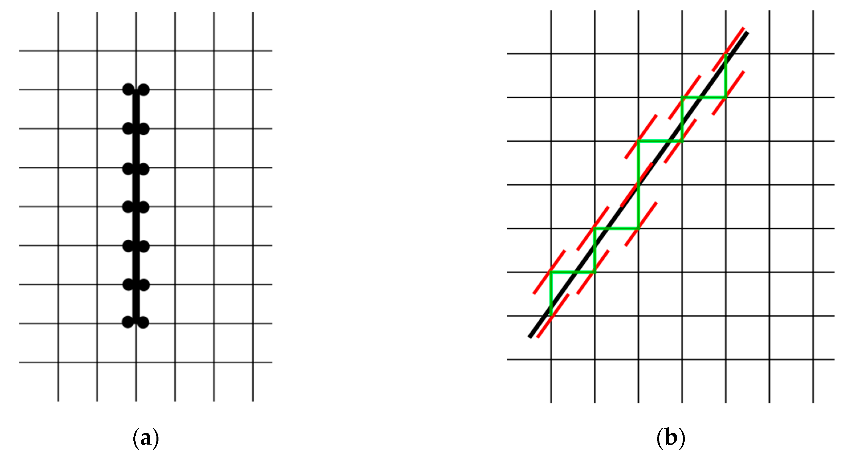
We propose a novel approach to modeling the inclined fractures on structural grids. The previously published methods [16,17] allow modeling in the case only, where the fracture boundary coincides with the cell boundaries (nodes) of the difference grid. In this work, we use two layers of nodes to explicitly define the fracture in order to correctly set the boundary conditions on the fracture [16].
The discretization scheme of such an algorithm is shown in Figure 1a. The fracture is indicated by a bold line, around it there is a fragmentation of the nodes of the computational grid used for the correct calculation of the boundary condition on Fracture (5). The novel approach assumes that the fracture does not coincide with the boundaries of the cells. Figure 1b schematically depicts an approach for identifying fractures in a grid. A fracture (thick black line) does not fall into the nodes of the grid. However, a discrete analogue of the fracture is considered (green line), which passes along the boundaries of the cells. Fracture is replaced by a bunch of tiny fractures scattering around it (red lines).
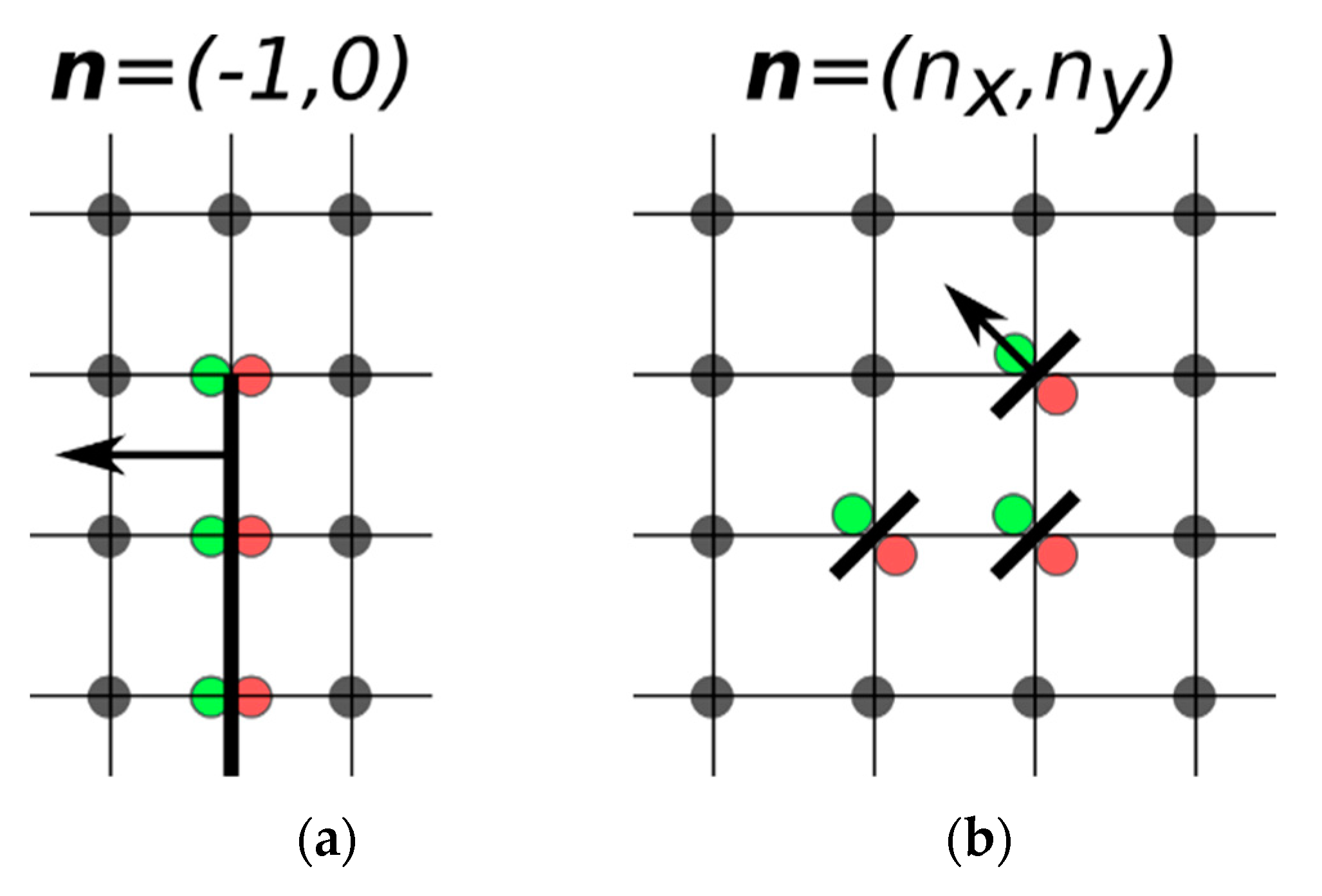
Figure 2 shows the calculation scheme of the boundary (contact) nodes near the fracture. In all cases, the nodes at the fracture boundary are duplicated.
In the case when the crack is aligned with the grid lines, the boundary conditions are calculated only along one axis (in the case in the figure along the x-axis). In the case of an inclined crack, the adjustment is made along two axes. In this case, information about the location of the fracture is lost, i.e., fracture turns out by a bunch of tiny fractures scattering around it and tied to grid points. This algorithm obviously has a drawback associated with the fact that the discretization of a fracture depends on the parameter of fineness of the mesh. However, it allows calculations on subvertical and inclined fractures, using the structural grids. Next, we compare these two methods.
5. Results
In this section, we present examples of calculations and a comparison of the proposed model with previously published results [16].
5.1. The Response from a Single Fracture: Fixed Fracture Position
The propagation of seismic waves from a source in a homogeneous medium with a fracture was simulated for the two-dimensional case. All calculations were carried out on rectangular structured grids. The source was located at a distance of 600 m from the center of the fracture. Five hundred receivers with a step of 1 m were located at a distance of 500 m from the center of the fracture. The homogeneous medium was a solid with a density of 2500 kg/m3, and the velocity of longitudinal and transverse waves were 3000 and 1400 m/s, respectively. A fracture 100 m long was located vertically in a homogeneous medium 2100 × 2100 m in size. At the top, bottom, and sides of the medium, the non-reflecting boundary conditions were set for the equivalence of the problem at different positions of the source-receiver system. The time step was 10−4 s. A 30 Hz Ricker pulse was used as a signal source. Grid size was 2100 × 2100, the computational time for one calculation was about 1200 s at a single core of modern Intel Core i7-7700K CPU (Intel, Santa Clara, CA, USA).
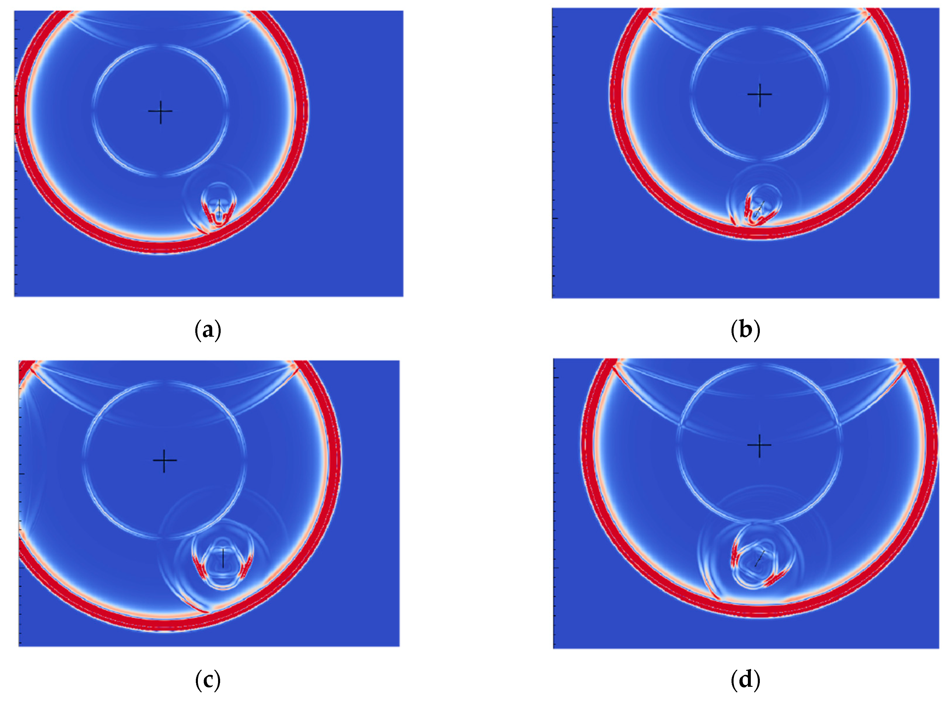
The calculation was carried out for two models: A vertical fracture directed along the grid axes and coordinate axes (Figure 3a) and an inclined fracture at an angle of 30°, modeled by the method proposed in this paper (Figure 3b). In the first case, the observation system was rotated relative to the fracture so that the models completely coincided when the coordinate system was rotated.
In all Figure 3a–d, the fracture is depicted in the center of the computational domain by a black line. The source is indicated by a black cross and is located directly above the source-receiver system (the black line is directly below the propagating wave). Figure 3a shows a wave for the initial setting of the source-receiver system relative to the fracture. In Figure 3b, the source-receiver system is located at an angle of 30° relative to its initial position (Figure 3a). In all wave patterns, wave reflections from the fracture are clearly visible.
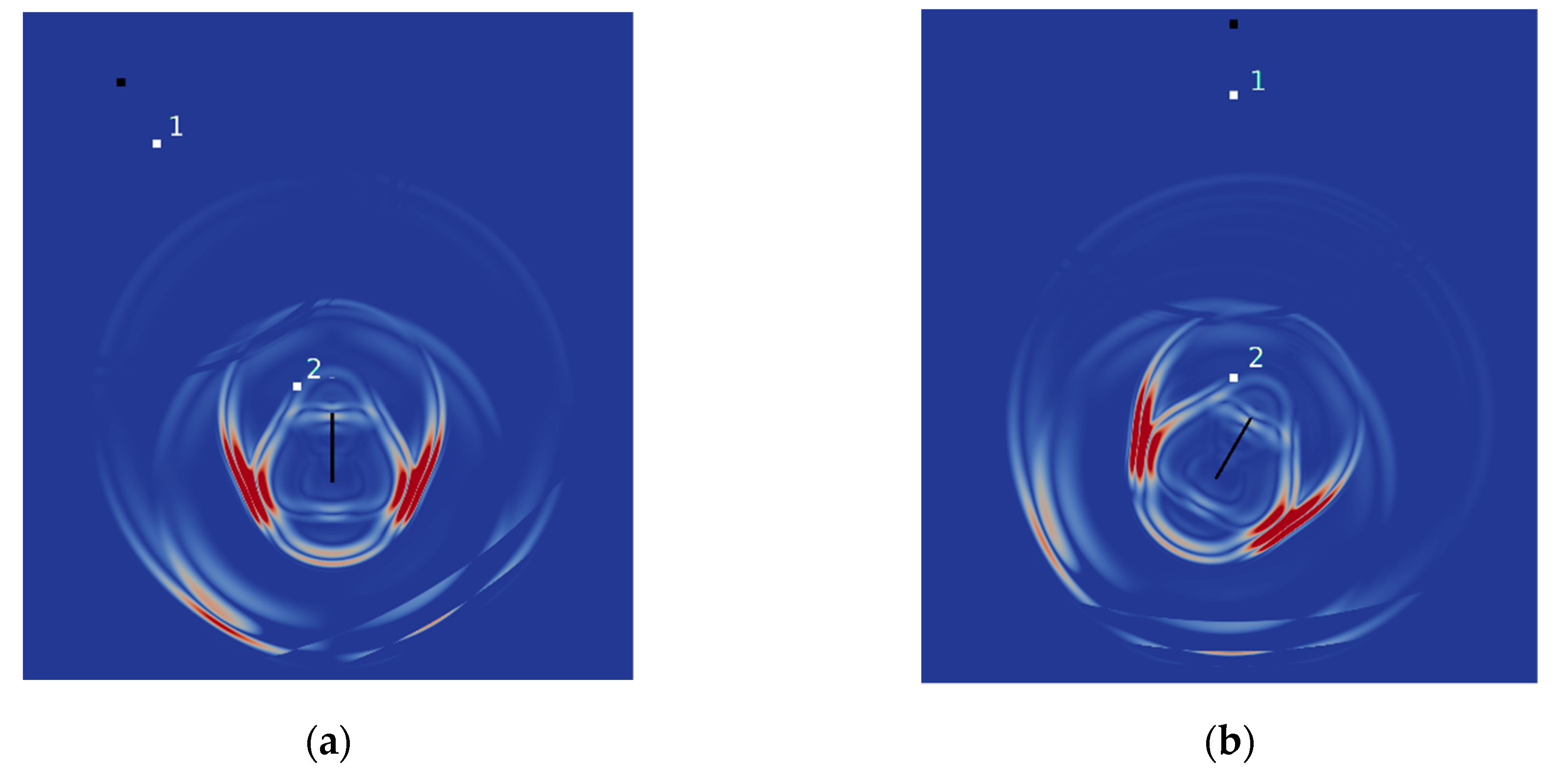
Figure 4 shows the wave field for the same calculation, but only the anomalous wave field from the fracture is displayed. The coincidence of responses is clearly seen from the figure.
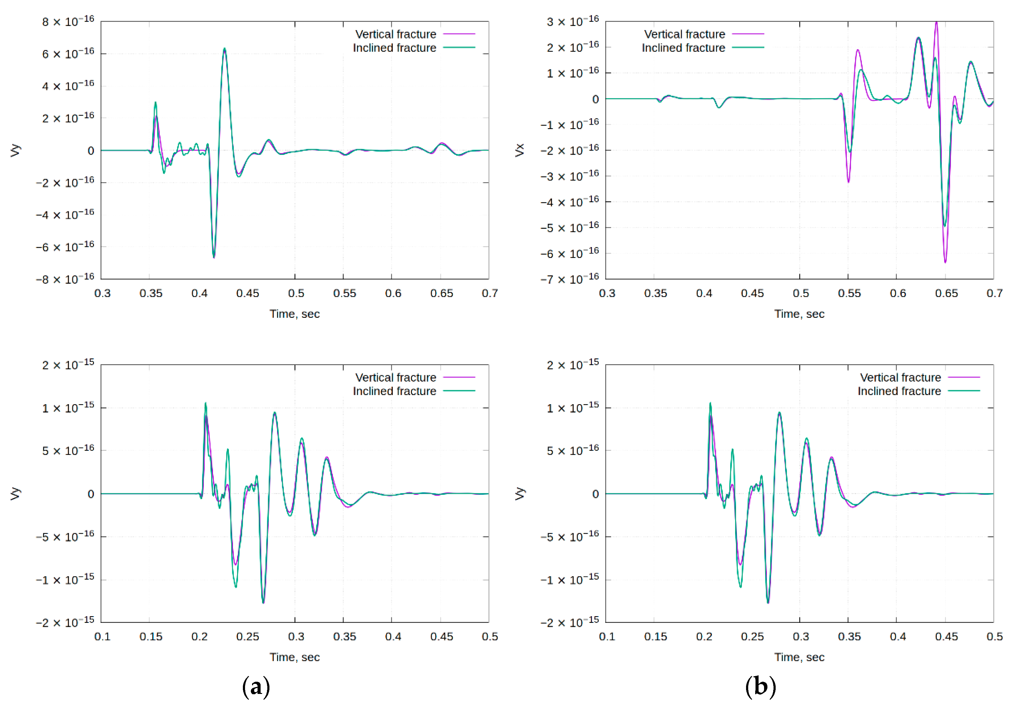
Figure 5 shows one-dimensional graphs of the values of the velocity components at one of the receivers versus time for two calculations. Only the anomalous field from the fracture is shown. The fracture is rotated at an angle of 30°. Figure 5a shows the field from the fracture on receiver 2, and Figure 5b shows the field from the fracture on receiver 2. A fairly good qualitative and quantitative agreement of the responses is seen. For the case of an inclined fracture in the time domain, t = 0.35–0.4 s “rattling” is observed due to the fact that the fracture structure is tied to discrete mesh cells. However, the main peak in the time domain is t = 0.4–0.45 s coincides and does not give a “rattle”. Further passage of the wavefront also coincides well for both settings.
5.2. The Response from a Single Fracture: Comparison with Unstructured Mesh
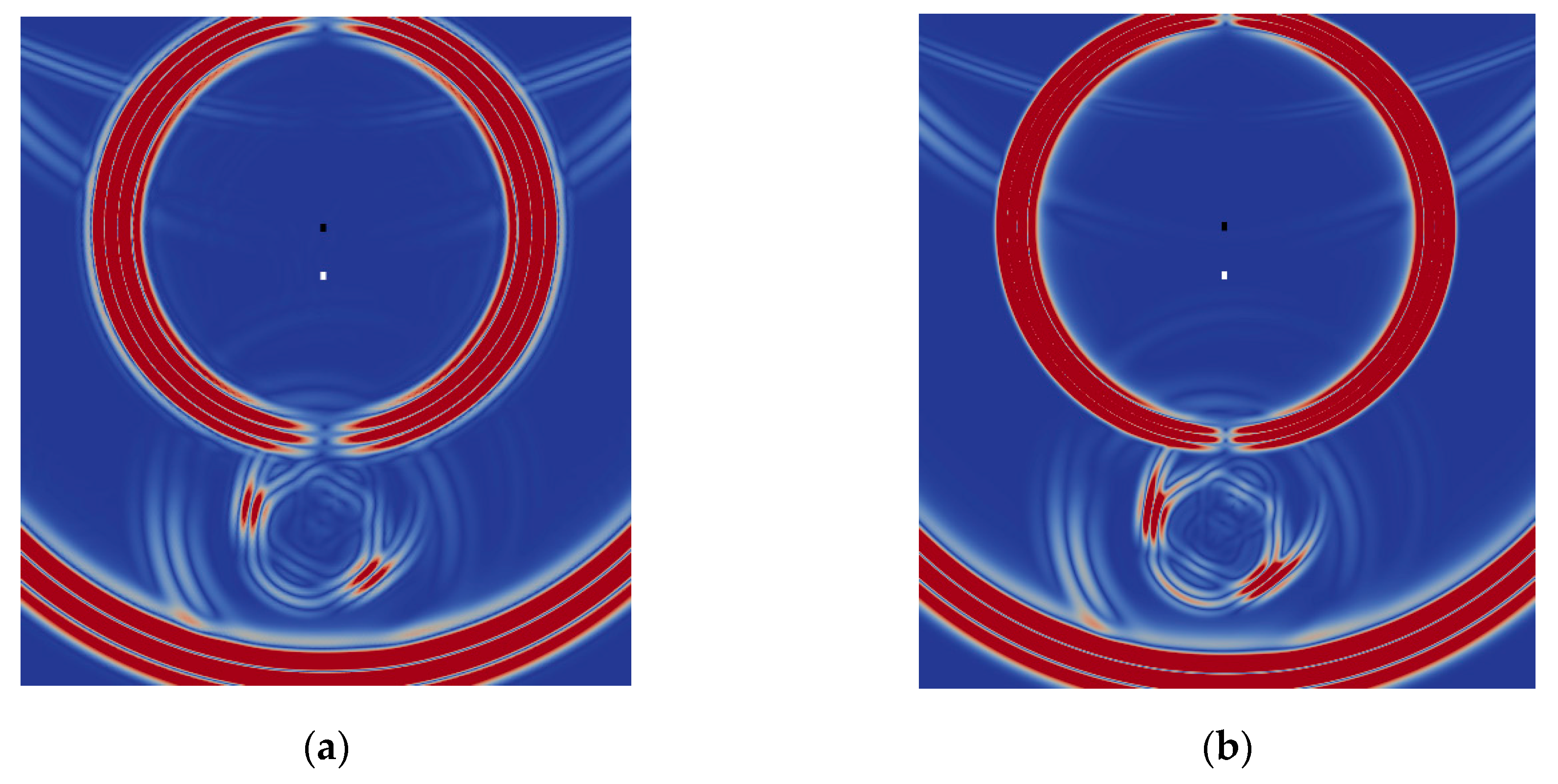
In this test, a model similar to the previous one was used with the 30° inclined fracture. The source was located at a distance of 600 m from the center of the fracture, the receiver was located at a distance of 500 m from the center of the fracture. The first calculation was carried out on structural grids using the grid-characteristic method and the fracture model proposed in this paper. The second calculation was carried out on unstructured mesh using the DG method. The wave snapshots are shown in Figure 6. The source position is shown by a black dot in the figure, the receiver by white a one. A 30 Hz Ricker pulse was used as a signal source. Unlike previous calculations, a directional source was used as the source (it was selected in connection with the features of the code for DG). It can be seen from the figure that the wave snapshots coincide qualitatively well. The response from the fracture has the same structure.
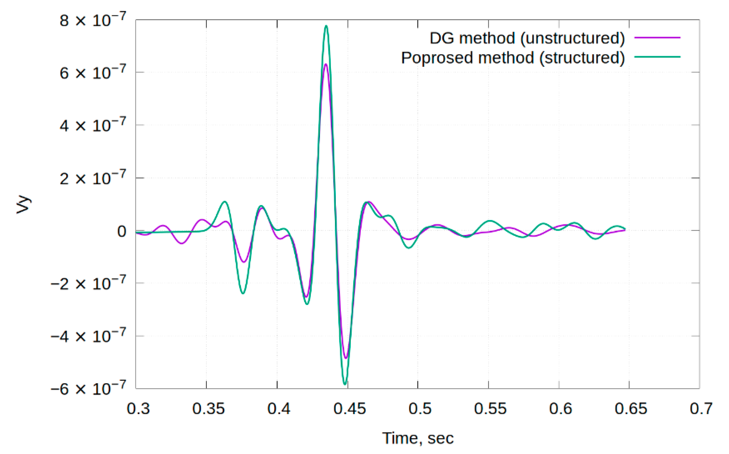
The distribution of the vertical velocity component at the receiver versus time is shown in Figure 7. Only a part of the signal is shown at time instants from 0.3 to 0.7 s, where there is a response from the fracture. The figure shows that the main response from the fracture coincides quite well. The arrival times are the same, the amplitude value is slightly different. The response from the fracture, calculated by the grid-characteristic method on structural grids is more “rattling”, this is due to the discrete geometry of the fracture model.
5.3. The Response from a Single Fracture: Calculation Errors Due to the Angle of Inclination
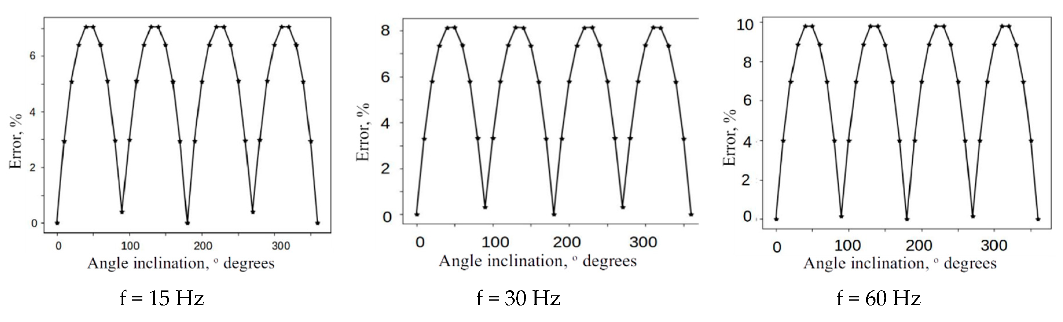
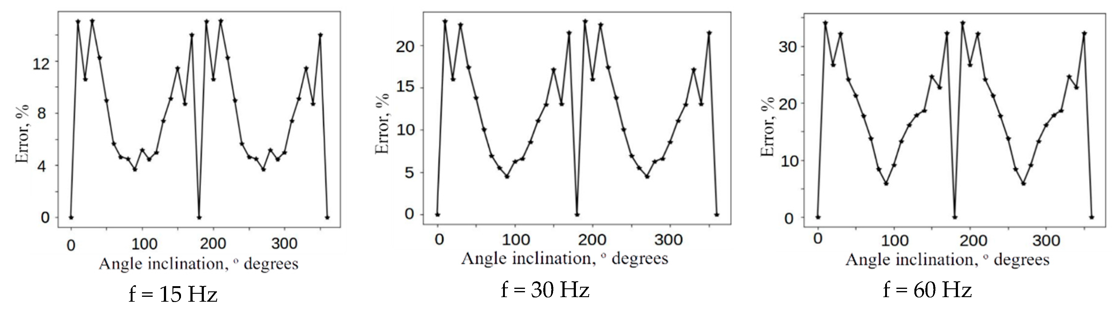
In the next series of calculations, the difference in the calculated responses was studied for the case of two scenarios. In the first scenario, a vertical fracture was used, and the observation system was rotated, in the second scenario, a fixed observation system was used and the fracture was rotated. The position of the fractures and observation systems was set in such a way that, when turning, all the systems coincided with each other. The initial setting was similar to the setting from the previous section. A series of calculations was carried out for various positions of the source-receiver system with a fixed position of the fracture in space. The source-receiver system for each new calculation was rotated relative to the fracture by 10° keeping the distance to the center of the fracture constant. In total, 35 calculations were performed with a step of 10° for various orientations of the source-receiver system relative to the fixed fracture. A similar series of calculations was carried out for different positions of the fracture with a fixed orientation of the source-receiver system. With each subsequent calculation, the fracture was rotated around its center by 10°. In total, 35 calculations were performed with a step of 10° for various fracture orientations. The differences between the obtained seismograms were studied when turning the source-receiver system with a fixed fracture and when turning a fracture with a fixed source-receiver system. Moreover, the influence of the source pulse frequency on the obtained errors in the seismograms was studied. A series of calculations were carried out for the following frequencies: 15, 30, 60 Hz. Grid size for each calculation was 2100 × 2100 nodes, spacing was 1 m.
Figure 8 shows the relative deviations in the decisions for the norm . Deviation was calculated by the formula
where is the value of velocity at the receiver; the error was summed over all receivers. From Figure 6, it follows that with decreasing frequency, the error decreases when the source-receiver system or fractures are rotated by the corresponding angle. At a frequency of 15 Hz, the maximum error (about 6.5%) is 1–2% less than the maximum error of the similar calculations at a frequency of 30 Hz (about 8%), which, in turn, is less than the maximum calculation error at a frequency of 60 Hz (about 10%). This result correlates well with the fact that with decreasing sampling size the error falls. Due to the fact that the new model of fractures is tied to the size of the cell, the longer waves produce a better result. Moreover, for fractures with a lower slope, the solutions have a smaller error.
Figure 9 shows a similar result for an anomalous field only (the field due to the fracture). The deviation values here are more significant, and they are associated with the discreteness of the inclined fracture. With increasing frequency, i.e., decreasing wavelength, the error increases. In Figure 5, peaks are visible that can give such a deviation in error; however, the qualitative coincidence of the waveform and the main peaks is quite good.
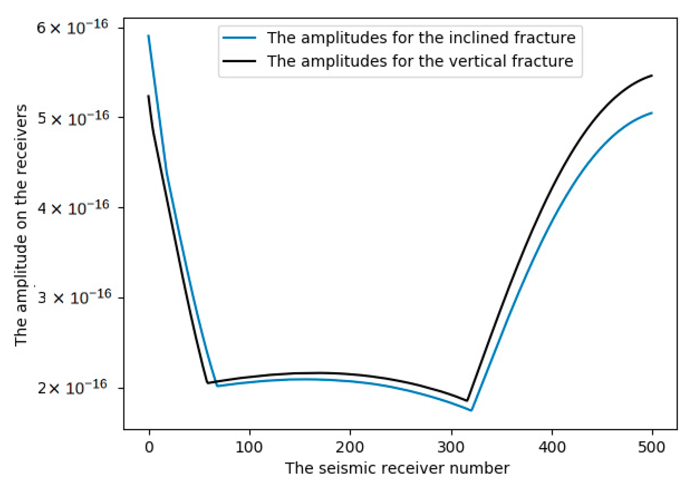
5.4. Single Fracture Response: Amplitude Study
Modern methods of interpretation increasingly take into account the absolute value of the amplitude of seismic signal, and not just the arrival times. As shown in Figure 5, the main peaks of the wave response from fractures come at the same time. Figure 10 shows the plots of the maximum amplitude of the seismic signal vs. the receiver number, based on the computations of the wave field reflections from the single fracture. We have compared the amplitudes of the seismic reflections from the inclined fracture under the angle of 30° with the amplitudes of the seismic reflections from the fracture, parallel to the boundaries of the grid. In our modeling study, 500 receivers of seismic signals were used. The blue line in Figure 10 denotes the peak amplitudes of the seismic reflections from the inclined fracture. The black line depicts the peak amplitudes of the seismic reflections from the vertical fracture, parallel to the boundaries of the grid cells. The plots show a similarity in the responses from the inclined and vertical structures.
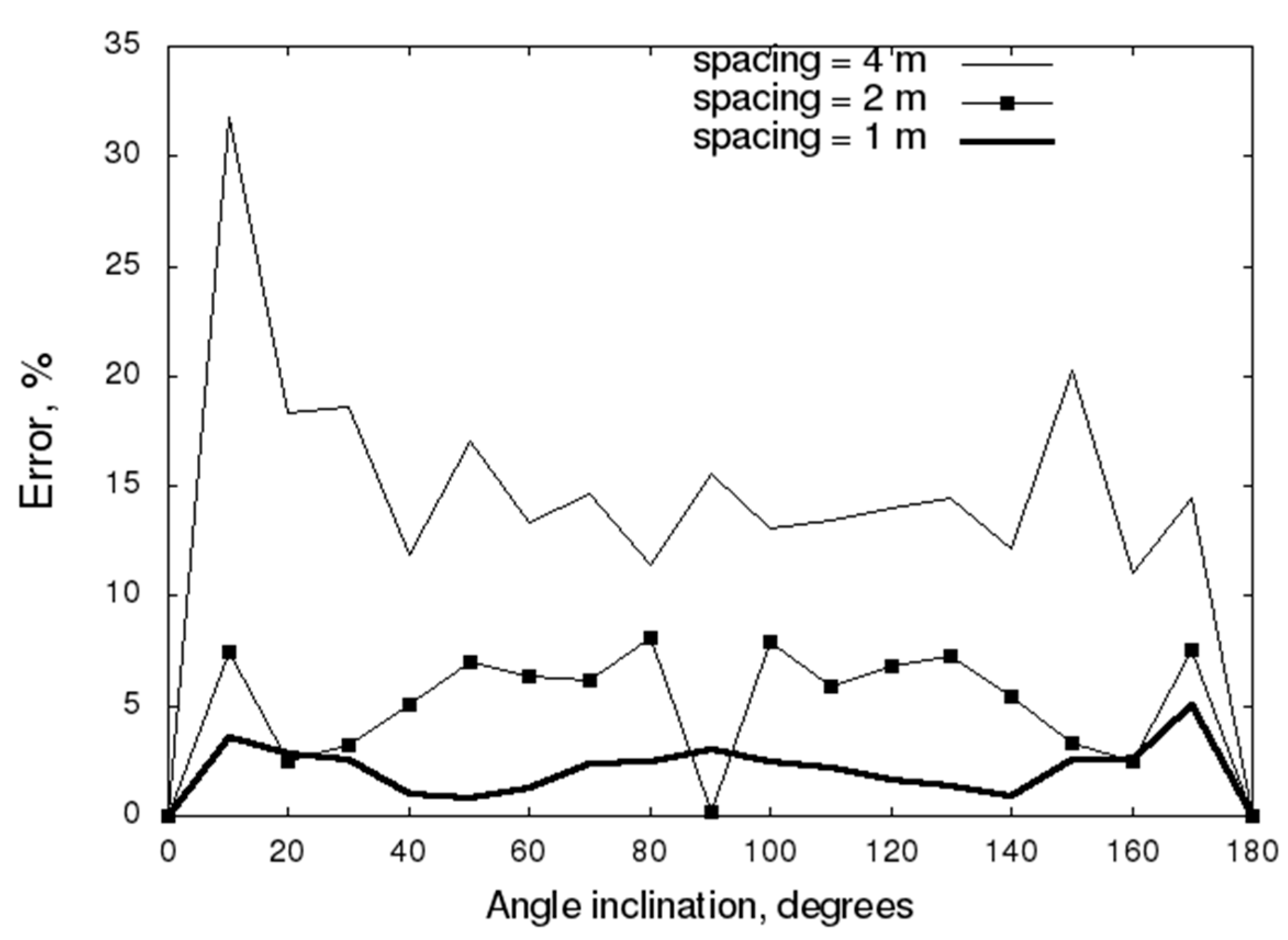
5.5. Single Fracture Response: Error Dependence on Grid Spacing
The next series of calculations investigates the dependence of the error from the grid step. The setting is similar to the previous ones, a vertical fracture was used, and the observation system was rotated, in the second scenario, a fixed observation system was used and the fracture was rotated. A series of calculations was carried out for various positions of the source-receiver system with a fixed position of the fracture in space. The source-receiver system for each new calculation was rotated relative to the fracture by 10° keeping the distance between the source-receiver system and the center of the fracture constant. In total, 19 calculations were performed with a step of 10° for various orientations of the source-receiver system relative to the fixed fracture. Source location is the same as shown in Figure 3 and Figure 4. The receiver is located at a distance of 100 m to the left of the center of the fracture. Source frequency is 30 Hz. A series of calculations was carried out for the grid spacing: 1, 2, 4 m. The calculation parameters are shown in Table 1.
Figure 11 shows the relative deviations in the decisions for the norm for various grid spacings.
For calculating the error, only the anomalous field from the fracture was used. The figure shows that with decreasing spacing, the error decreases. Based on this, we can assume that there is a grid convergence of the method.
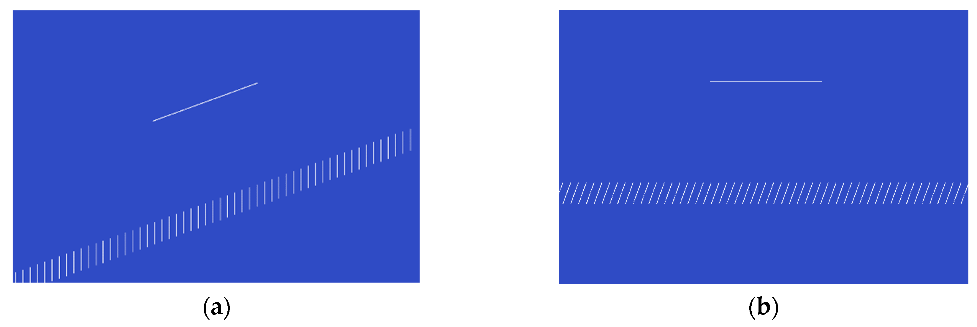
5.6. Response from a Cluster of Subvertical Fractures
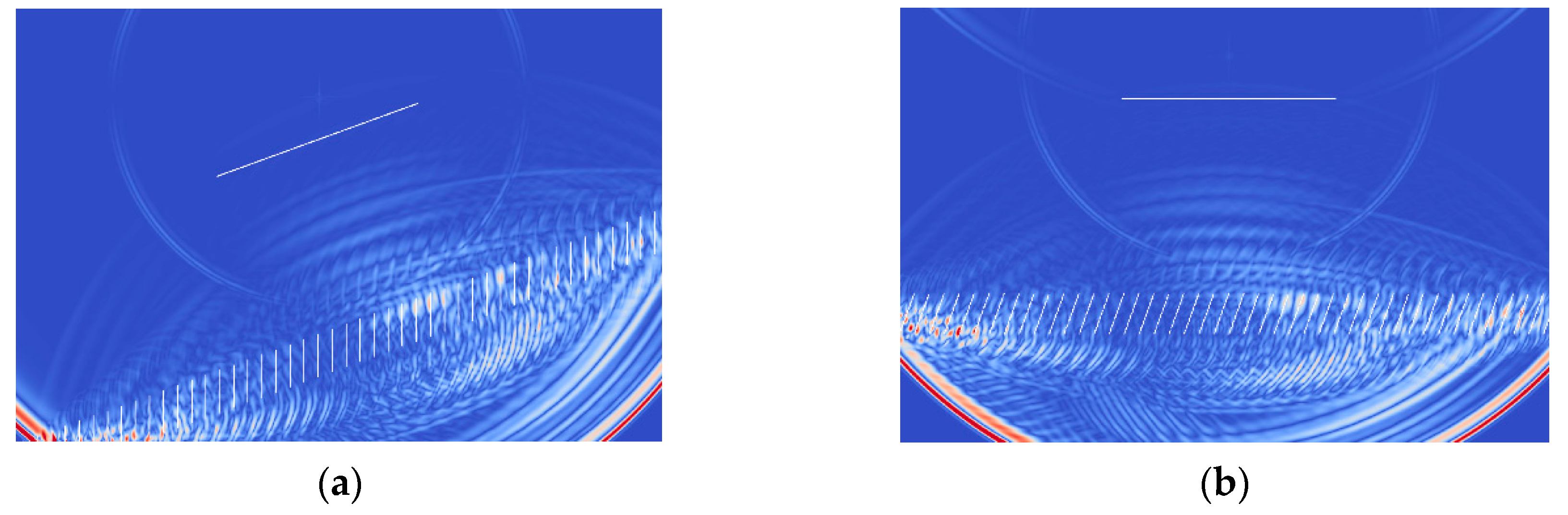
The computations of the wave field reflections from a cluster of the parallel fractures were carried out. In the first case, the fractures were inclined at an angle of 20°, and the system of receivers and source of impulse were parallel to the boundaries of the grid (Figure 12a). In the second case, the fractures were parallel to the boundaries of the modeling grid, and the system of receivers and source of impulse were inclined at an angle of 20° (Figure 12b).
The seismic reflections from the cluster of the parallel fractures are shown in Figure 13. The overall wave reflections from the fractures are similar if we rotate the coordinate system of the model in Figure 12a under the angle of 20°, which is the angle of the inclined fractures.
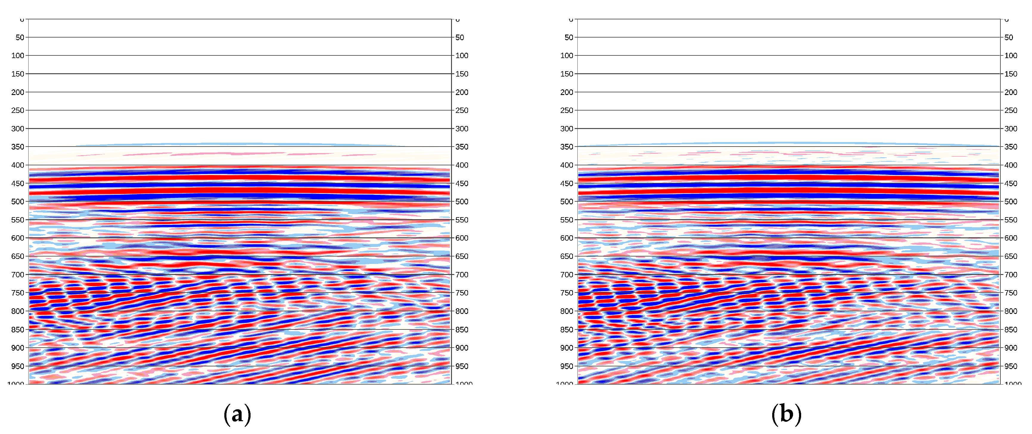
Figure 14 shows the seismograms of the vertical velocity components at the receivers for two models. Only the anomaly part of the response is given. The same color scale is used. A good qualitative and quantitative agreement of responses is observed. The first response has the largest amplitude and is clearly visible on seismograms.
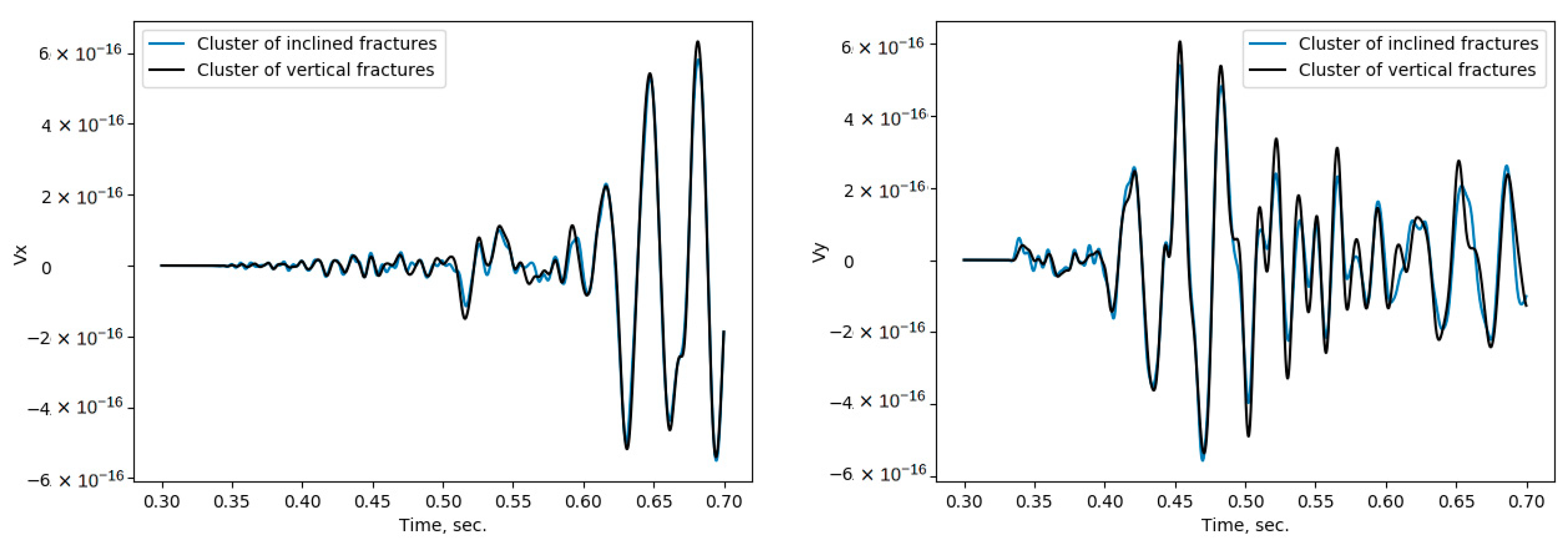
Figure 15 shows the recording from the central receiver for the vertical and horizontal velocity components.
A good qualitative and quantitative agreement of the result for the two methods is observed.
6. Discussion and Conclusions
This paper presents a novel approach to modeling the elastic field propagation in a medium containing the clusters of subvertical fractures. The new approach is based on the use of the grid-characteristic method [16]. Unlike previously proposed methods, this method can be used for modeling the seismic responses from subvertical fractured inhomogeneities on a structural rectangular grid. This greatly simplifies the construction of the numerical model and the use of the algorithms. The shortcomings of the proposed methodology include the fact that the crack model is discrete and does not take into account the normal of the crack. The crack is replaced by a discrete analog presented by a bunch of tiny fractures scattering around it and tied to grid points. At each point, the normal is taken into account, the total field due to interference gives a response close to real. In addition, in the case of an inclined crack, the initial grid does not change and the position of the crack can be set only up to the position of the grid node, respectively, there is an error where is the grid spacing. A comparison of the new approach with the traditional method shows that the results produced by both methods agree well with each other. The wave fields for a cluster of the inclined fractures and a cluster of the vertical fractures demonstrate a similar behavior. Thus, the results of the numerical study demonstrate that the developed method provides an effective tool for modeling the elastic field propagation in the fractured geological media. This method can be used in interpretation of the seismic data in the areas with complex fractured geological structures typical for mineral deposits and the HC reservoirs.
We proposed this method as a method for quick analysis and preliminary calculations of fractured geological models. Its advantages include:
- Fairly quick calculation and simple implementation in a structural grid. The basic calculation algorithm does not change; the method is implemented as a “corrector” step.
- The ability to calculate inclined fractures on structural grids.
- The ability to build a fractured inhomogeneity of complex shape.
- The absence of the need to build an unstructured mesh, the binding of the grid to inhomogeneity.
- Fractures can be easily added at any place in the geological models.
- The disadvantages include:
- A rather large integral error.
- Substantial grid spacing reduction required to reduce error.
The use of structural or non-structural grids to calculate dynamic wave disturbances in geological models is an open discussion. It was shown in [19] that methods on structural grids work up to 100 times faster than a method on unstructured ones. The authors of [27] also say that the use of finite-element methods and the DG method is more computationally difficult than finite difference methods. Implementation of finite-elements and DG requires an unstructured mesh, which should accurately approximate at least the main interfaces of the model. Construction of such a mesh is a problem of high complexity, which is hard to parallelize and requires manual quality control. Methods on structural grids are quite easy to parallel [23] and quite effective in both CPU [28] and GPU [29].
It should be noted that this approach is quite easily transferred to the three-dimensional case. The grid-characteristic method uses splitting in spatial coordinates, and the transition from the 2D to 3D case is quite simple. Further studies in this direction may be related to transitions to the three-dimensional case. The authors are working in this direction.
Author Contributions
Conceptualization, N.K.; methodology, N.K. and P.S.; software, N.K.; validation, P.S.; formal analysis, P.S.; investigation, N.K.; resources, P.S.; data curation, P.S.; writing—original draft preparation, N.K. and P.S.; writing—review and editing, N.K. and P.S.; visualization, P.S.; supervision, N.K.; project administration, N.K.; funding acquisition, N.K. All authors have read and agreed to the published version of the manuscript.
Funding
This research was supported by the Russian Science Foundation, project No. 16-11-10188.
Acknowledgments
This work has been carried out using computing resources of the federal collective usage center Complex for Simulation and Data Processing for Mega-science Facilities at NRC “Kurchatov Institute”, http://ckp.nrcki.ru/.
Conflicts of Interest
The authors declare no conflict of interest.
References
- Karayev, N.; Levyant, V.; Petrov, I.; Karayev, N.; Muratov, M. Assessment by methods mathematical and physical modelling of possibility of use of the exchange scattered waves for direct detection and characteristics of systems of macrocracks. Seism. Technol. 2015, 1, 22–36. [Google Scholar]
- Schoenberg, M. Elastic Wave Behavior across Linear Slip Interfaces. J. Acoust. Soc. Am. 1980, 68, 1516. [Google Scholar] [CrossRef] [Green Version]
- Hsu, C.; Schoenberg, M. Elastic Waves through a Simulated Fractured Medium. Geophysics 1993, 58, 964–977. [Google Scholar] [CrossRef]
- Dablain, M.A. The application of high-order differencing to the scalar wave equation. Geophysics 1986, 51, 54–66. [Google Scholar] [CrossRef]
- Moczo, P.; Robertsson, J.O.A.; Eisner, L. Advances in Wave Propagation in Heterogeneous Earth. Adv. Geophys. 2007, 48, 1–606. [Google Scholar]
- Komatitsch, D.; Vilotte, J.P. The spectral element method: an efficient tool to simulate the seismic response of 2D and 3D geological structures. Bull. Seismol. Soc. Am. 1998, 88, 368–392. [Google Scholar]
- Chaljub, E.; Komatitsch, D.; Vilotte, J.-P.; Capdeville, Y.; Valette, B.; Festa, G. Spectral element analysis in seismology. Adv. Geophys. 2007, 48, 365–419. [Google Scholar]
- Dumbser, M.; Kaser, M. An Arbitrary High Order Discontinuous Galerkin Method for Elastic Waves on Unstructured Meshes II: The Three-Dimensional Isotropic Case. Geophys. J. Int. 2006, 167, 319–336. [Google Scholar] [CrossRef]
- Pan, G.; Abubakar, A. Iterative solution of 3D acoustic wave equation with perfectly matched layer boundary condition and multigrid preconditioner. Geophysics 2013, 78, T133–T140. [Google Scholar] [CrossRef]
- Belonosov, M.; Dmitriev, M.; Kostin, V.; Neklyudov, D.; Tcheverda, V. An iterative solver for the 3D Helmholtz equation. J. Comput. Phys. 2017, 345, 330–344. [Google Scholar] [CrossRef]
- Malovichko, M.S.; Khokhlov, N.I.; Yavich, N.B.; Zhdanov, M.S. Parallel integral equation method and algorithm for 3D seismic modelling. In Proceedings of the 79th EAGE Conference and Exhibition, Paris, France, 12–15 June 2017. [Google Scholar] [CrossRef]
- Malovichko, M.S.; Khokhlov, N.I.; Yavich, N.B.; Zhdanov, M.S. Acoustic 3D modeling by the method of integral equations. Comput. Geosci. 2018, 111, 223–234. [Google Scholar] [CrossRef]
- Cui, X.; Lines, L.R.; Krebes, E.S. Seismic Modelling for Geological Fractures. Geophys. Prospect. 2018, 66, 157–168. [Google Scholar] [CrossRef] [Green Version]
- Bosma, S.; Hajibeygi, H.; Tene, M.; Tchelepi, H.A. Multiscale Finite Volume Method for Discrete Fracture Modeling on Unstructured Grids (MS-DFM). J. Comput. Phys. 2017, 351, 145–164. [Google Scholar] [CrossRef]
- Franceschini, A.; Ferronato, M.; Janna, C.; Teatini, P. A Novel Lagrangian Approach for the Stable Numerical Simulation of Fault and Fracture Mechanics. J. Comput. Phys. 2016, 314, 503–521. [Google Scholar] [CrossRef]
- Kvasov, I.; Petrov, I. Numerical Modeling of Seismic Responses from Fractured Reservoirs by the Grid-Characteristic Method; Leviant, V., Ed.; Society of Exploration Geophysicists: Tulsa, OK, USA, 2019. [Google Scholar] [CrossRef]
- Cho, Y.; Gibson, R.L.; Lee, J.; Shin, C. Linear-Slip Discrete Fracture Network Model and Multiscale Seismic Wave Simulation. J. Appl. Geophys. 2019, 164, 140–152. [Google Scholar] [CrossRef]
- Vamaraju, J.; Sen, M.K.; De Basabe, J.; Wheeler, M. Enriched Galerkin Finite Element Approximation for Elastic Wave Propagation in Fractured Media. J. Comput. Phys. 2018, 372, 726–747. [Google Scholar] [CrossRef]
- Biryukov, V.A.; Miryakha, V.A.; Petrov, I.B.; Khokhlov, N.I. Simulation of Elastic Wave Propagation in Geological Media: Intercomparison of Three Numerical Methods. Comput. Math. Math. Phys. 2016, 56, 1086–1095. [Google Scholar] [CrossRef]
- Mercerat, E.D.; Glinsky, N. A Nodal High-Order Discontinuous Galerkin Method for Elastic Wave Propagation in Arbitrary Heterogeneous Media. Geophys. J. Int. 2015, 201, 1101–1118. [Google Scholar] [CrossRef] [Green Version]
- Miryaha, V.A.; Sannikov, A.V.; Petrov, I.B. Discontinuous Galerkin Method for Numerical Simulation of Dynamic Processes in Solids. Math. Model. Comput. Simulations 2015, 7, 446–455. [Google Scholar] [CrossRef]
- Favorskaya, A.V.; Zhdanov, M.S.; Khokhlov, N.I.; Petrov, I.B. Modelling the Wave Phenomena in Acoustic and Elastic Media with Sharp Variations of Physical Properties Using the Grid-Characteristic Method. Geophys. Prospect. 2018, 66, 1485–1502. [Google Scholar] [CrossRef]
- Ivanov, A.M.; Khokhlov, N.I. Efficient Inter-Process Communication in Parallel Implementation of Grid-Characteristic Method. Springer: Cham, Switzerland, 2019; pp. 91–102. [Google Scholar] [CrossRef]
- Golubev, V.I.; Khokhlov, N.I. Estimation of Anisotropy of Seismic Response from Fractured Geological Objects. Comput. Res. Model. 2018, 10, 231–240. [Google Scholar] [CrossRef] [Green Version]
- Ruzhanskaya, A.; Khokhlov, N. Modelling of Fractures Using the Chimera Grid Approach. In Proceedings of the 2nd Conference on Geophysics for Mineral Exploration and Mining, Belgrade, Serbia, 9–13 September 2018. [Google Scholar] [CrossRef]
- Stognii, P.; Khokhlov, N.; Zhdanov, M. Novel Approach to Modelling the Elastic Waves in a Cluster of Subvertical Fractures. In Proceedings of the 81th EAGE Conference and Exhibition, London, UK, 3–6 June 2019. [Google Scholar] [CrossRef]
- Lisitsa, V.; Cheverda, V.; Botter, C. Combination of the discontinuous Galerkin method with finite differences for simulation of seismic wave propagation. J. Comput. Phys. 2016, 311, 142–157. [Google Scholar] [CrossRef]
- Furgailo, V.; Ivanov, A.; Khokhlov, N. Research of Techniques to Improve the Performance of Explicit Numerical Methods on the CPU. In Proceedings of the 2019 Ivannikov Memorial Workshop (IVMEM), Velikiy Novgorod, Russia, 13–14 September 2019; pp. 79–85. [Google Scholar] [CrossRef]
- Khokhlov, N.; Ivanov, A.; Zhdanov, M.; Petrov, I.; Ryabinkin, E. Applying OpenCL Technology for Modelling Seismic Processes Using Grid-Characteristic Methods; Springer: Cham, Switzerland, 2016; pp. 577–588. [Google Scholar] [CrossRef]
Figure 1.
The discretization schemes illustrating different approaches to modeling a single fracture on a structural grid. Figure (a) shows the approach when the fracture is aligned with the grid cells [7,8]. The new approach (b) implies that the fracture is inclined.

Figure 2.
The layout of the contact nodes of the calculation grid. Red and green dots indicate duplicate nodes from one and the other side of the fracture. The left picture (a) is shown for the case when the fracture is aligned with the grid lines, the right picture (b) is for an inclined fracture.
Figure 2.
The layout of the contact nodes of the calculation grid. Red and green dots indicate duplicate nodes from one and the other side of the fracture. The left picture (a) is shown for the case when the fracture is aligned with the grid lines, the right picture (b) is for an inclined fracture.

Figure 3.
Fracture wave responses computed using two approaches. Figure (a,c) shows the wave for the initial setting of the source-receiver system relative to the fracture. On (b,d), the source-receiver system is located at an angle of 30° relative to its initial position.
Figure 3.
Fracture wave responses computed using two approaches. Figure (a,c) shows the wave for the initial setting of the source-receiver system relative to the fracture. On (b,d), the source-receiver system is located at an angle of 30° relative to its initial position.

Figure 4.
Anomalous wave field from the fracture for two approaches. Figure (a) shows the wave for the initial formulation of the source-receiver system relative to the fracture. In (b), the source-receiver system is located at an angle of 30° relative to its initial position. The black dot denotes the source location, white dots depict the location of the first and second receivers, respectively.

Figure 5.
The value of the velocity components at one of the receivers versus time for two calculations. Only the anomalous field from the fracture is shown. Figure (a) shows the field from the fracture on receiver 2, and figure (b) shows the field from the fracture on receiver 1.
Figure 5.
The value of the velocity components at one of the receivers versus time for two calculations. Only the anomalous field from the fracture is shown. Figure (a) shows the field from the fracture on receiver 2, and figure (b) shows the field from the fracture on receiver 1.

Figure 6.
Fracture wave responses computed using two approaches. A fracture is depicted in the center of the computational region. Figure (a) shows the wave for the DG (Discontinuous Galerkin) method on unstructured mesh, (b) for purposed method on structured mesh.
Figure 6.
Fracture wave responses computed using two approaches. A fracture is depicted in the center of the computational region. Figure (a) shows the wave for the DG (Discontinuous Galerkin) method on unstructured mesh, (b) for purposed method on structured mesh.

Figure 7.
The value of the velocity component at one of the receivers versus time for two calculations.
Figure 7.
The value of the velocity component at one of the receivers versus time for two calculations.

Figure 8.
Relative deviation of the norm of errors for two calculations depending on the angle of rotation of the fracture and on the frequency of the signal.
Figure 8.
Relative deviation of the norm of errors for two calculations depending on the angle of rotation of the fracture and on the frequency of the signal.

Figure 9.
Relative deviation of the norm of errors for two scenarios depending on the angle of rotation of the fracture and on the frequency of the signal.
Figure 9.
Relative deviation of the norm of errors for two scenarios depending on the angle of rotation of the fracture and on the frequency of the signal.

Figure 10.
Peak amplitudes of the seismic signal on the receivers for the inclined fractures and for the vertical fractures.
Figure 10.
Peak amplitudes of the seismic signal on the receivers for the inclined fractures and for the vertical fractures.

Figure 11.
Relative deviation of the norm of errors for two scenarios depending on the angle of rotation of the fracture and on the frequency of the signal. The result is shown for three grid spacings: 1, 2, 4 m.
Figure 11.
Relative deviation of the norm of errors for two scenarios depending on the angle of rotation of the fracture and on the frequency of the signal. The result is shown for three grid spacings: 1, 2, 4 m.

Figure 12.
The schematic representation of the models with the cluster of parallel fractures. Panel (a) shows a model with the inclined receivers under 20°, and a cluster of fractures parallel to the boundaries of the grid cells. Panel (b) presents the model with the cluster of the inclined fractures under 20° and the receivers parallel to the boundaries of the grid cells.

Figure 13.
Wave field reflections from the cluster of parallel fractures. (a) The wave field from the cluster of fractures, parallel to the boundaries of the grid cells. (b) The wave field from the cluster of the inclined fractures under 20° boundaries.
Figure 13.
Wave field reflections from the cluster of parallel fractures. (a) The wave field from the cluster of fractures, parallel to the boundaries of the grid cells. (b) The wave field from the cluster of the inclined fractures under 20° boundaries.

Figure 14.
Vertical velocity component seismograms at receivers for a cluster of parallel fractures. An anomaly field is displayed. (a) The seismogram from the cluster of fractures, parallel to the boundaries of the grid cells. (b) The seismogram from the cluster of the inclined fractures under 20°.

Figure 15.
Velocity components of seismograms at single central receivers for a cluster of parallel fractures. An anomalous field is displayed.
Figure 15.
Velocity components of seismograms at single central receivers for a cluster of parallel fractures. An anomalous field is displayed.


Table 1.
Calculation parameters.
| Grid Spacing, m | Grid Size | Time Steps | Time Step, s | Cells Per Wavelength | Calculation Time, s |
|---|---|---|---|---|---|
| 1 | 2100 × 2100 | 5000 | 10−4 | ~46 | 1180 s |
| 2 | 1050 × 1050 | 2500 | 2 × 10⁻⁴ | ~23 | 157 s |
| 4 | 525 × 525 | 1250 | 4 × 10⁻⁴ | ~11 | 15 s |
© 2020 by the authors. Licensee MDPI, Basel, Switzerland. This article is an open access article distributed under the terms and conditions of the Creative Commons Attribution (CC BY) license (http://creativecommons.org/licenses/by/4.0/).
Share and Cite
MDPI and ACS Style
Khokhlov, N.; Stognii, P. Novel Approach to Modeling the Seismic Waves in the Areas with Complex Fractured Geological Structures. Minerals 2020, 10, 122. https://0-doi-org.brum.beds.ac.uk/10.3390/min10020122
AMA Style
Khokhlov N, Stognii P. Novel Approach to Modeling the Seismic Waves in the Areas with Complex Fractured Geological Structures. Minerals. 2020; 10(2):122. https://0-doi-org.brum.beds.ac.uk/10.3390/min10020122
Chicago/Turabian StyleKhokhlov, Nikolay, and Polina Stognii. 2020. "Novel Approach to Modeling the Seismic Waves in the Areas with Complex Fractured Geological Structures" Minerals 10, no. 2: 122. https://0-doi-org.brum.beds.ac.uk/10.3390/min10020122
Note that from the first issue of 2016, this journal uses article numbers instead of page numbers. See further details here.