
Torque Analysis of a Gyratory Crusher with the Discrete Element Method


1
Department of Mechanical Engineering, University of Concepción, Edmundo Larenas 219, Concepción 4070409, Chile
2
Department of Metallurgical Engineering, University of Concepción, Edmundo Larenas 285, Concepción 4070371, Chile
*
Author to whom correspondence should be addressed.
Minerals 2021, 11(8), 878; https://0-doi-org.brum.beds.ac.uk/10.3390/min11080878
Submission received: 18 June 2021
/
Revised: 5 August 2021
/
Accepted: 9 August 2021
/
Published: 13 August 2021
(This article belongs to the Special Issue Simulation Using the Discrete Element Method (DEM) in the Minerals Industry)
Abstract
:Comminution by gyratory crusher is the first stage in the size reduction operation in mineral processing. In the copper industry, these machines are widely utilized, and their reliability has become a relevant aspect. To optimize the design and to improve the availability of gyratory crushers, it is necessary to calculate their power and torque accurately. The discrete element method (DEM) has been commonly used in several mining applications and is a powerful tool to predict the necessary power required in the operation of mining machines. In this paper, a DEM model was applied to a copper mining gyratory crusher to perform a comprehensive analysis of the loads in the mantle, the crushing torque, and crushing power. A novel polar representation of the radial forces is proposed that may help designers, engineers, and operators to recognize the distribution of force loads on the mantle in an easier and intuitive way. Simulations with different operational conditions are presented and validated through a comparison with nominal data. A calculation procedure for the crushing power of crushers is presented, and recommendations for the selection of the minimum resolved particle size are given.
1. Introduction
Comminution is the progressive reduction in size of run-of-mine (ROM) ore, and its initial stage is consists of primary crushing [1]. Gyratory crushers are the most common machine used in the primary crushing in the copper mining industry of Chile and worldwide, and they are designed for large tonnage throughput. Notably, Chile has produced almost one-third of global copper mine production, and this industry is one of the most important industries for this country [2].
Currently, there is a strong interest to study the operating parameters of primary and secondary crushers in order to optimize their performance [3]. For this reason, different models have been developed to predict the operating conditions of gyratory crushers. These models can be classified as empirical [4] and mechanistic models [5,6]: of the latter, some of them can be solved numerically, such as with the discrete element method.
The discrete element method (DEM) is an explicit numerical scheme utilized to simulate the dynamical behavior of granular flow. The interaction of the particles is monitored contact by contact, and the motion is modeled for each particle [7]. It was first proposed by Cundall [8], and then it was expanded to three dimensions by Hart and Cundall [9,10]. The particles in the system interact with one another through forces calculated by contact models, allowing the computation of the interactions between particles and between particles and walls. For all the time steps, the equations of motion for each particle are numerically solved, and the new position of the particles is acquired and updated for the new time step.
DEM has been used by engineers and scientists in an extensive range of fields, in particularly, DEM has become one of the most important tools for simulating the behavior of machines and processes in mineral processing and grinding [11]. DEM simulations deliver dynamic information, such as the transient forces for each particle, that is extremely complicated if not impossible to obtain through physical experiments with current scientific and experimental development [12]. To simulate comminution equipment, it is necessary to use a proper breakage model to represent the particle size distribution (PSD) of the progeny particles and the specific energy consumption.
Several gyratory and cone crushers have been simulated with DEM. Litcher et al. proposed a two-way coupling DEM-PBM (Population Balance Model) model of cone crushers [13], where the PBM was used to represent the size reduction in the particles. A B90 cone crusher and a HP100 cone crusher were simulated, and the particle size distribution of the product was validated. Li et al. [14] presented a DEM model of a cone crusher by using the particle replacement method (PRM) to represent the breakage of rocks. They studied the effect of closed side setting and eccentric speed on the size distribution of the products with DEM simulations. Delaney et al. [15] simulated an industrial-scale cone crusher with DEM employing super-quadrics particles, and a DEM breakage model was proposed where the particles were broken when the contact energy reaches a maximum value. The progeny size distribution of this breakage model was obtained with data from the Julius Kruttschnitt Mineral Research Centre (JKRMC) Drop Weight Test. Quist et al. [16] investigated an industrial-scale Svedala H6000 cone crusher using DEM and experiments. The commercial software EDEM 2.5 (provided by DEM Solutions Ltd., Edinburgh, Scotland, UK) was employed with a bonded particle model (BPM) to describe the particle breakage. Throughput capacity, power draw, and product particle size distribution were calculated in the simulations and then compared with experimental data. For throughput capacity, relative errors of 34.6% and 1.97% were obtained for closed side settings equal to 34 mm and 50 mm, respectively. Using the same DEM code, Johansson et al. [3] presented a DEM simulation of a Morgårdshammar B90 laboratory cone crusher, and the results were compared with laboratory experiments. Two case simulations had been performed for investigating the influence of eccentric speed at 10 Hz and 20 Hz. The PSD of the product matched the experimental results relatively well with the corresponding coarse region. Comparing the mass flow rate, a relative error of 1.36% was achieved for the simulation at 10 Hz, and 56.4% was achieved for the simulation at 20 Hz. Chen et al. performed a DEM simulation and parameter optimization of a gyratory crusher by utilizing the bonded-particle model to represent particle breakage [17]. These simulations were performed with the EDEM software in a CG810i SANDVIK gyratory crusher, and a full sensibility analysis was accomplished. André and Tavares published simulations of a laboratory-scale cone crusher by adopting a novel breakage model [18]. Their results provided good agreement with experiments for throughput with a relative error of 9.6, 10.4, and 37.9% for the three cases presented, but the findings reported a deviation up to a 50% for specific energy and product size. A multibody dynamic and discrete element method was presented to analyze the performance of the GYP1200 inertia cone crusher, and it was contrasted with experimental data, obtaining a 4% of relative error in both power draw and throughput for the 400 rpm case, 11% error in power draw, and a 22% error in throughput for the 600 rpm case [19]. Complete research of comminution modeling was presented by Cleary et al., focusing on recent advances in particle-based modeling of crushing [20]. Three machines were analyzed: twin roll crusher, cone crusher, and vertical shaft impactor (VSI). Between the challenges that they proposed, an industrial-scale validation of DEM models of crushers is highlighted. A crushing chamber optimization with DEM (EDEM 2018) was performed by using a genetic algorithm [21]. The particle breakage was modeled by BPM, modeling the particles as a cube shape ore of 300 mm of edge formed by spherical particles of 30 mm of radius. After the optimization, an increase of 36% and 26% was reported in productivity and power density (mass flow rate per unit of power), respectively. Another chamber optimization was performed by adopting a dual-objective optimization of productivity and product quality in a C900 cone crusher [22]. The productivity was determined with an analytical model and numerically with DEM. Optimization of the angular speed of the mantle consisted of the following: the length of the parallel zone; the bottom angle of the mantle; the eccentric angle; the eccentricity; and the engagement angle. The productivity and the percentage of crushed products were increased by about 2% and 2.1%, respectively.
In this paper, a Metso 60-110 gyratory crusher of 1500 kW nominal power operating in a Chilean copper mine is modeled and simulated by using the discrete element method in order to study the crushing power and crushing torque under different operational conditions. The software Rocky DEM is employed with polyhedral particles, a hysteretic contact model, and the Tavares’ breakage model [23]. The simulations are validated by utilizing the nominal and experimental data of throughput, product size, and crushing power, being an important contribution to comminution modeling [20]. A complete force analysis of the loading force distribution acting on the crusher’s mantle and the torque in the mantle geometry is performed with a moving frame of reference in polar coordinates. With this variable change, a planar force and torque distribution can be obtained, as can be observed in a previous work [21] and machines such as jaw crushers [24]. As a novelty, a calculation procedure for the crushing power of crushers is proposed where the torque is computed with radial forces because only these forces are transmitted to the eccentric.
2. Gyratory Crusher
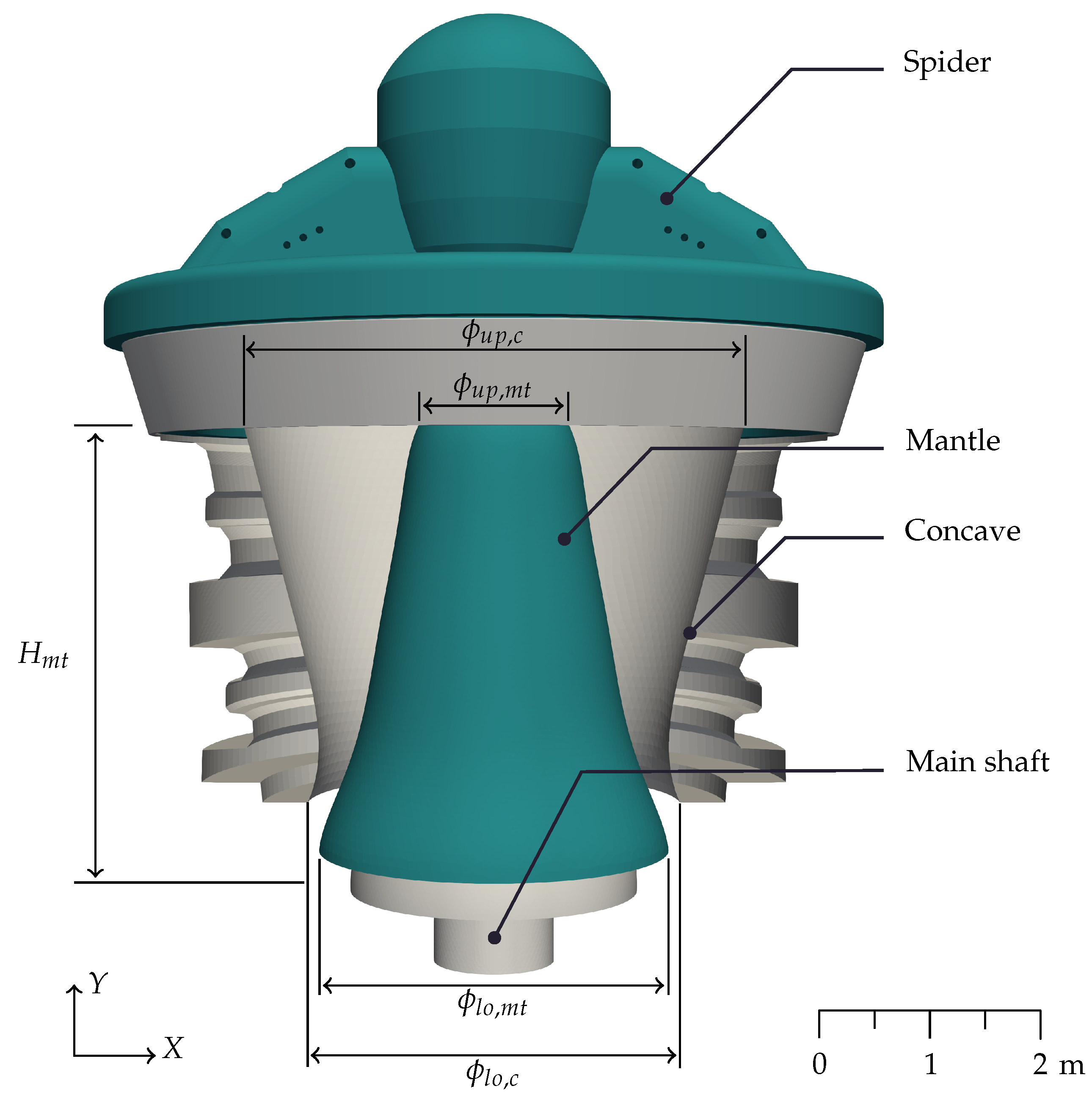
A gyratory crusher consists of a movable and truncated conical head and a fixed concave shell, as is presented in Figure 1. The head is integral with the main shaft, and it is covered by an element of wear named mantle. The set of these parts is the main shaft assembly. The external element is denominated concave and is fixed on the main frame of the machine. The main shaft is supported by the spider at the top and by the main shaft position system (a hydraulic system of vertical adjustment) and eccentric bushing at the bottom.
The functional principle of the machine is to compress the ore among the mantle and the concave. To achieve particle compression, the main shaft rotates eccentrically, allowing a periodic approach and receding of the mantle regarding the concave. This means that, for a given angular and vertical position, the distance between the mantle and the concave periodically changes with each rotation of the main shaft. The eccentric, as its name indicates, allows the eccentric motion. This motion is produced by an electric motor coupled to the pinion shaft, which is connected to the eccentric by a helical gear.
The closed side setting, , is defined as the smallest distance between the mantle and the concave, and the open side setting, , is defined as the greatest distance at the same height [16]. Due to the eccentric motion, if at a given vertical position this distance is the , the will be in the diametrically opposite position. The rotational speed of the eccentric is between 85 and 150 rpm [25].
The classical empirical approach to estimate the crushing power, P, is by using Equation (1), derived from Bond’s equation [26]:
where is the mass flow rate of the product, is a constant of the machine, is the work index, and and are the size of the cumulative percentage lower to 80% in the product and feed, respectively. The power draw is obtained by adding the no-load power, which can be measured empirically.
On the other hand, by utilizing data from DEM simulations, the crushing power can be calculated with the contact information between particles and the mantle in terms of the crushing torque [16]. In the same manner as Bond’s equation, the no-load or idle power must be added to the crushing power in order to obtain the overall power to operate this machine [27].
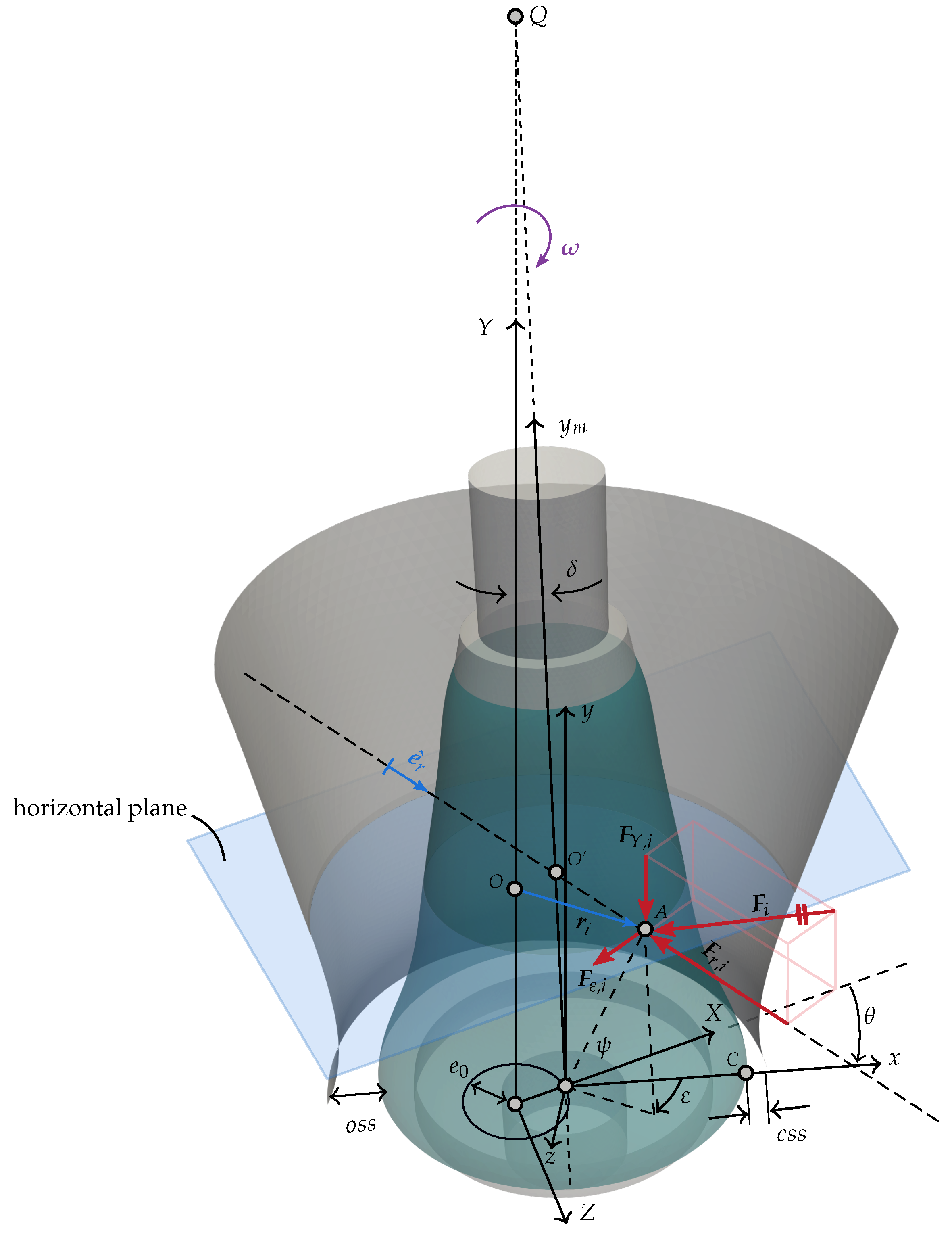
Let us consider a force between a particle and the mantle applied in the i-node or point A of the mantle, as can be observed in Figure 2 where all the following geometrical parameters are shown in that illustration. A fixed and a moving frame of reference are used. The frame follows the motion of the main shaft rotating at the same speed and with , where t is time. The Y-axis is the axis of the eccentric, and the -axis is the axis of the main shaft. A polar coordinate system is also utilized, where is measured regarding the x-axis and the is always at or point C. The position of point A is represented with the vector and angles and .
The contact force is decomposed into three components: , , and . The radial r and transverse components are the projection in a horizontal plane of the contact force between the particle and the mantle in polar coordinates. The Y-component is the vertical component of this force.
As the main shaft is mounted in a full lubricated eccentric bushing, the power and torque needed to break the ore are evaluated only with the particle-mantle radial force, . The torque produced by the transverse forces, , on the mantle is not transmitted to the eccentric assembly and only produces a rotation about the main shaft’s axis, which is also called head spin, [3]. Radial forces are those that compress the particles. The vertical force is supported by the main shaft position system, and it does not produce torque.
The dashed line presented in Figure 2 graphically represents the radial direction, which joins the intersection between the main shaft’s axis and the horizontal plane, point and point A. This direction is mathematically expressed with the unit vector, ; therefore, the radial component in the horizontal plane of the contact force is as follows:
Subsequently, the crushing torque, T, in the Y-axis of the N nodes of the mantle in the instant t is calculated with the following equation:
where is the vector starting at point O and finishing at point A. Point O corresponds to the intersection between the horizontal plane and the central axis of the eccentric, which is the Y-axis. Then, by using the definition of work expressed with torque and the angular speed in the Y-axis of the eccentric being equal to , the crushing power is described as follows:
If the angular speed is constant, the crushing power, , is only time-dependent in terms of the crushing torque, . Gyratory crushers operate when it reaches the constant angular speed and with a frequency converter; consequently, the angular velocity in operation is generally constant.
In some DEM applications such as ball mill [28], jaw crusher [24], high pressure roll grinding [29,30], agitated drum dryer [31], V-blender [32], and screw conveyor [33], the calculation of power draw is expressed by the sum of the scalar product of the force applied on the i-node and the velocity vector of the same node, , with the following expression:
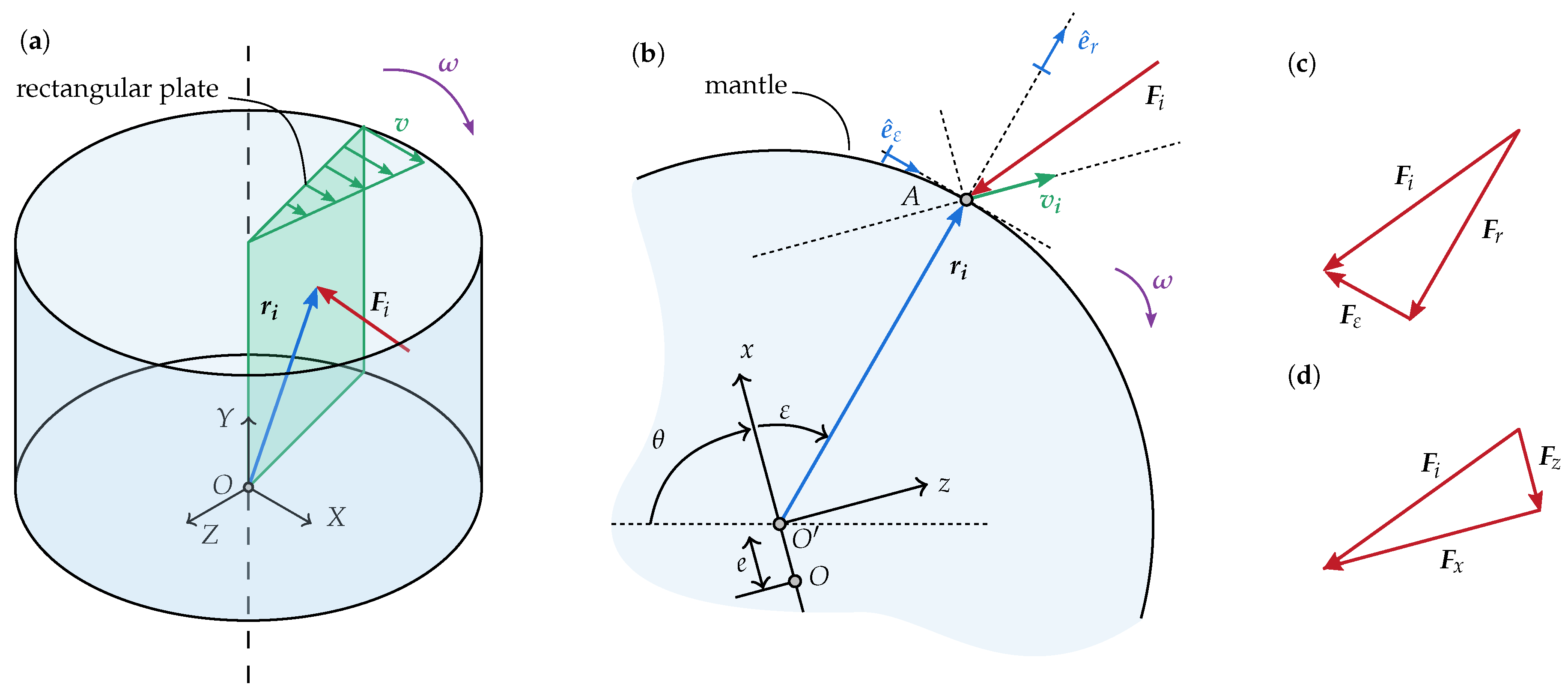
Notwithstanding, the definitions of power with force (4) and torque (5) are equivalent, Equation (5) is not correct for gyratory crushers since it considers the tangential forces and head spin. If we consider a simple case of a rectangular plate rotating around a vertical axis Y as the mixer shown in Figure 3a, both Equations (4) and (5) deliver the same result because only forces perpendicular to the rectangular plate provides work. By knowing that the torque is and that the velocity of any point in the plate is equal to and is perpendicular to the rectangular plate, the statement can be verified.
For gyratory crushers, if we use (5), the power will consider the work performed by transverse forces. Figure 3b presents a part of a cross-section of the mantle at a height Y. A force vector applied on the mantle and the velocity, , of the i-node is provided. If the head spin is null, the velocity is the same in all cross-sections of the mantle, perpendicular to the x-axis, and with magnitude equal to , where e is the eccentricity at that height Y. As the velocity is parallel to the z-axis, only the component in the same axis performs work, ; therefore, by utilizing Equation (5), the crushing power will be described as follows:
Figure 3c,d describes the rectangular decomposition of the contact force in radial and transverse direction, and x and z, respectively. A change in the transverse component will generate a variation in the z-component. As depends on the transverse component of the contact force, the power calculation with Equation (5) will consider the work of transverse forces; thus, it is not convenient for this application and the power will be overestimated.
Furthermore, if the head spin is not null, the velocity in the node i changes to , changing the magnitude and direction of the velocity of the node. This change in the direction of the velocity will affect the scalar product of (4), and consequently that equation is not recommended.
The polar coordinate system proposed in Figure 2 can be used to analyze the torque produced by radial forces over the mantle. With the geometry presented in Figure 3b we can define the following:
where r is the mantle’s radius, and and belong to the x-axis and z-axis, respectively. Then, the crushing torque (3) in polar coordinates is expressed as in Equation (10).
As e is a function of the height Y, Equation (10) depends on r and . With that expression, we can find the maximum and minimum of the torque by considering the contact force as constant. A critical point was not observed by studying the first partial derivative regarding and r. By analyzing the boundary, it was found that the torque was maximum in and , and it was minimum in and , where is the maximum radius of the mantle located at the bottom. Moreover, there is a change in the sign of the torque. If we consider the torque positive in , in the torque will be negative. Besides, from (10) it is possible to note that the torque is zero for and because the moment arm of the radial force is null.
3. DEM Model
In the discrete element method, particles and boundaries are simulated, such as rigid bodies. Contact forces are modeled as damping spring systems by considering an overlap distance between them. The normal contact force is modeled with the hysteretic linear spring model proposed by Walton and Braun [34] and the linear spring Coulomb limit for the tangential component of the force. The implementation of the normal contact model in Rocky is time-dependent, as described by the following set of equations for the time step j:
where and are the normal elastic-plastic contact forces at the current time, , and at the previous time, , respectively. is the change in the contact normal overlap during the current time. and are the normal overlap values at the current and at the previous time, respectively. and are the values of loading and unloading contact stiffnesses, respectively.
is a dimensionless stabilization constant parameter; its value in Rocky DEM is 0.001. The use of ensures that, during the unloading, the normal force will return to zero when the overlap decreases to zero.
The tangential forces, , are represented by the linear spring Coulomb limit model:
where is the tangential force given by (14), and is the coefficient of friction. The following is described:
with being the value of the tangential force at the previous time, denotes the tangential relative displacement of the particles during the time step, and is the tangential stiffness. The stiffnesses can be calculated as is described in Appendix A.1 in accordance with the material parameters.
For the purpose of establish the normal and tangential direction in contact, a contact plane is utilized, and the normal direction is thereby perpendicular to that plane. For example, the contact plane in the interaction between two spherical particles is defined as the plane perpendicular to the line that connects the centers of these particles. For polyhedral particles, the particle–boundary contact algorithm uses the closest points of the particle and a triangle of the meshed boundary or two points with the maximum overlap distance to create a line and then a plane perpendicular to this line [34].
To accurately describe the physical phenomenon in the gyratory crusher, a breakage model is needed to ensure particle flow through the machine. In the selected software, there are two of these models: Ab-T10 and Tavares. Both models are a particle replacement scheme (PRM), changing the polyhedral parent particle in polyhedral progeny particles, and preserve both mass and volume in the resulting fragments in a breakage event. The Tavares model is selected to represent the breakage of the particles because it has extensive material characterization. This breakage model can characterize body breakage of polyhedral convex particles, and the particles will break in depending on the energy dissipated in a contact when they are under stress [23]. If the energy is not enough to break the particle, the particle will weaken, decreasing its strength.
The fragments of a broken particle are generated following the Voronoi fracture algorithm [35] according to a size distribution. Rocky has two different models available for the size distribution: Gaudin–Schumann and incomplete beta function [36]. The last one was selected in this work, and the details of the calculation procedure of the breakage model are presented in Appendix A.2.
4. Simulation
Simulations were performed by using the software Rocky DEM version 4.2.0 (provided by ESSS Chile SpA, Santiago, Chile) on The Southern GPU-cluster with 2 GPU per task. Each simulation took about 15 to 30 days, and the size of the simulation results is between 2 and 4 TB. Both variables depend on the simulation conditions. One of the reasons for the high simulation time and storage is the high sampling frequency of 2500 Hz used.
The geometry and movement of the boundaries, the material and breakage parameters, and the conditions of the simulations are presented in the following subsections.
4.1. Geometry
The Metso 60-110 gyratory crusher was 3D modeled in an open-source mesh generator software (Gmsh 4.8.4 developed by Christophe Geuzaine and Jean-François Remacle, Belgium) by using the available data on the website of the manufacturer, and the main parameters used are listed in Table 1. Only the parts in contact with the particles are modeled: the main shaft, mantle, concave, and spider, as shown in Figure 1. The mantle is modeled with a smooth profile. Splines were used for better characterization of mantle and concave curvatures. It is easy to compute, by using mathematical functions of the geometries, the linear relationship between the , , and height of the main shaft [37]. Moreover, the crusher feed hopper was modeled to achieve a more realistic representation of the ore falling into the crushing chamber (or crusher cavity) and settling in it.
To describe the movement of the main shaft, this geometry was firstly tilted at an angle relative to its pivot point Q. Then, a rotation around the vertical Y-axis of angular speed, , is defined. This movement is described as a periodic rotation motion in the software. In these conditions, the eccentricity at the base of the mantle is 46.6 mm. Free body rotation of the mantle about the -axis is also set to consider the effect of the tangential forces of the particles on the mantle. This feature allows us to obtain a head spin in an ideal condition when there are no tangential forces (or are negligible) at the bottom support due to the bushing in perfect condition and optimal lubrication. As the manufacturer indicates, in most cases, the no-load head spin is less than 20 rpm, and an excessively worn spider bushing will increase its value. The inertia of main shaft is needed to calculate the free body rotation; thus, by using the CAD model, the mass and inertia were obtained, as is indicated in Table 1. The mantle bottom diameter is 3.3 m, and the height is 4.0 m. The mean side angle of the mantle is 100° relative to the horizontal. The concave bottom diameter is 3.5 m.
The definition of the normal direction and the application point of the force in the particle-boundary contact is important in this research since both parameters changed the resulting crushing torque. A coarse mesh of the boundaries drastically changes the results of the crushing torque because the direction of the force and moment arm can be affected; thus, a fine mesh of the mantle with a triangle size of 20 mm is used, which is close to the minimum particle size utilized in these DEM simulations.
4.2. Material Parameters
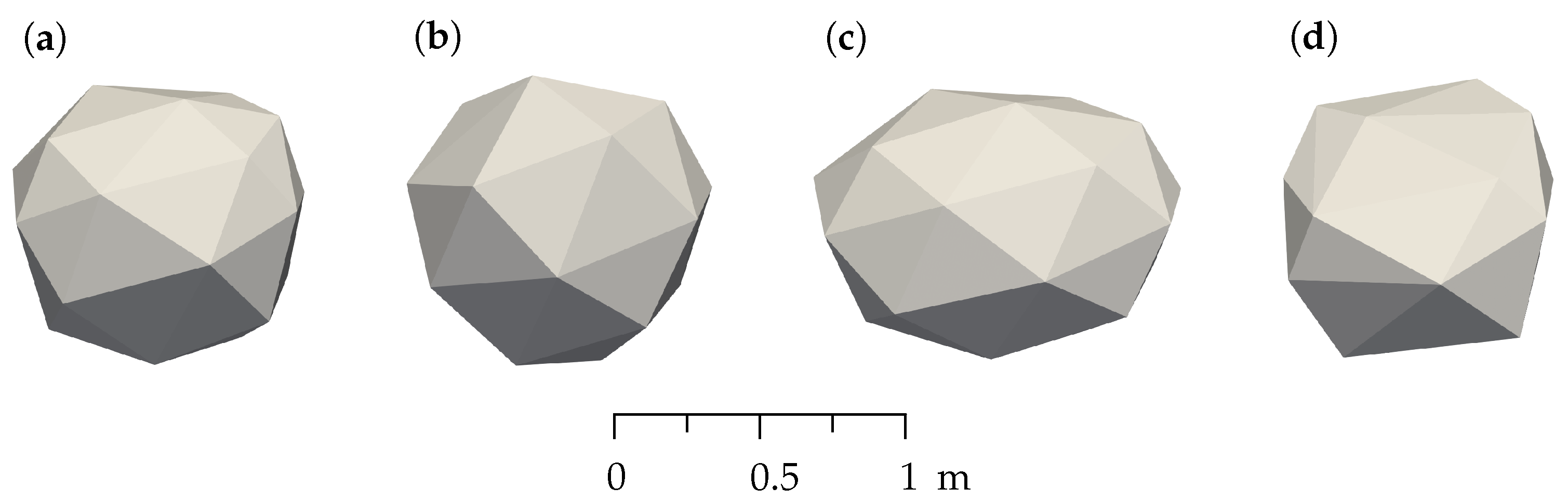
The ROM ore copper was simulated using polyhedral particles with four different shapes that are represented by a vertical aspect ratio, a horizontal aspect ratio, number of corners, and a super-quadric degree. These parameters were selected by André and Tavares [18] and are representative of the real shape of the rocks. The simulated particles are presented in Figure 4, where the presented scaled size of these particles is the maximum size used in this work. The Tavares breakage model is used, which has shown a good response when simulating different types of ore [18,23]. The material and breakage parameters of the particles of copper ore used in this work were adjusted by Tavares et al. [23] and can be observed in Table 2 and Table 3. The work index, , is 13.5 kWh/t [23]. The feed particle size distribution utilized is characterized by mm and was selected according to the recommendation of the manufacturer and considers a reasonable simulation time. The smallest particle size in the feeding is 70 mm with 39.42% in mass. Despite being a large size compared to the fine particles found experimentally, it can well represent the physical situation.
The minimum resolved particle size, , considered in the simulation is 10 mm, which is the lower particle size than can be generated in a fracture event, i.e., for a particle smaller than this threshold, breakage is not allowed. The selection of must ensure an accurate particle size distribution of the product. In a unidimensional simulation of compression of soils, , which is also called comminution limit, was set proportional to by using a of 0.25 [38,39]. Utilizing the same criteria, in a model of a split Hopkinson pressure bar test, a ratio of 0.22 was selected [40]. With this relationship and a feeding size of mm, the minimum particle size should be mm. Zhou et al. [41] suggest calculating with the maximum particle size as . With the maximum particle size in the feeding equaling m, the minimum particle size should be mm. Andre and Tavares [18] proposed to use as one-tenth of the representative size. They employed the geometric mean of the feed size range as the characteristic size. By using the representative size as , a minimum particle size of 51.65 mm is obtained.
Given that the computed with the preceding approaches is quite high, we propose that instead of using the size of the feeding as a reference, a representative size of the product must be used in comminution models. By selecting the as the parameter to represent the product size distribution, the ratio of the minimum simulated size is defined as the minimum valid closed side setting divided by the minimum simulated particle size as follows.
The ratio in previous research works of gyratory and cone crushers is quite low, which means the smallest particle is close to the . Most of them have , and the maximum value is 7.08 [16], as presented in Table 4. For simulations where BPM was used, the is considered as the minimum size of the fraction particles. Unresolved particles were presented by researchers of CSIRO, allowing a particle up to 0.5 mm to be obtained in the product size distribution, but they are not in the DEM simulation [15,20,42]. Using a will be enough to ensure good results in the simulations, and it is viable in terms of simulation times. In this work, the minimum is 111.62 mm, thus, . Even though it is well known that the breakage of smaller particles produces an increase in torque, many authors use larger sizes in order to reduce the simulation time. The results do not qualitatively change [42]. Choosing a lower size provides better resolution in the particle size, but results in higher computational costs relative to both simulation times and storage.
4.3. Simulation Conditions
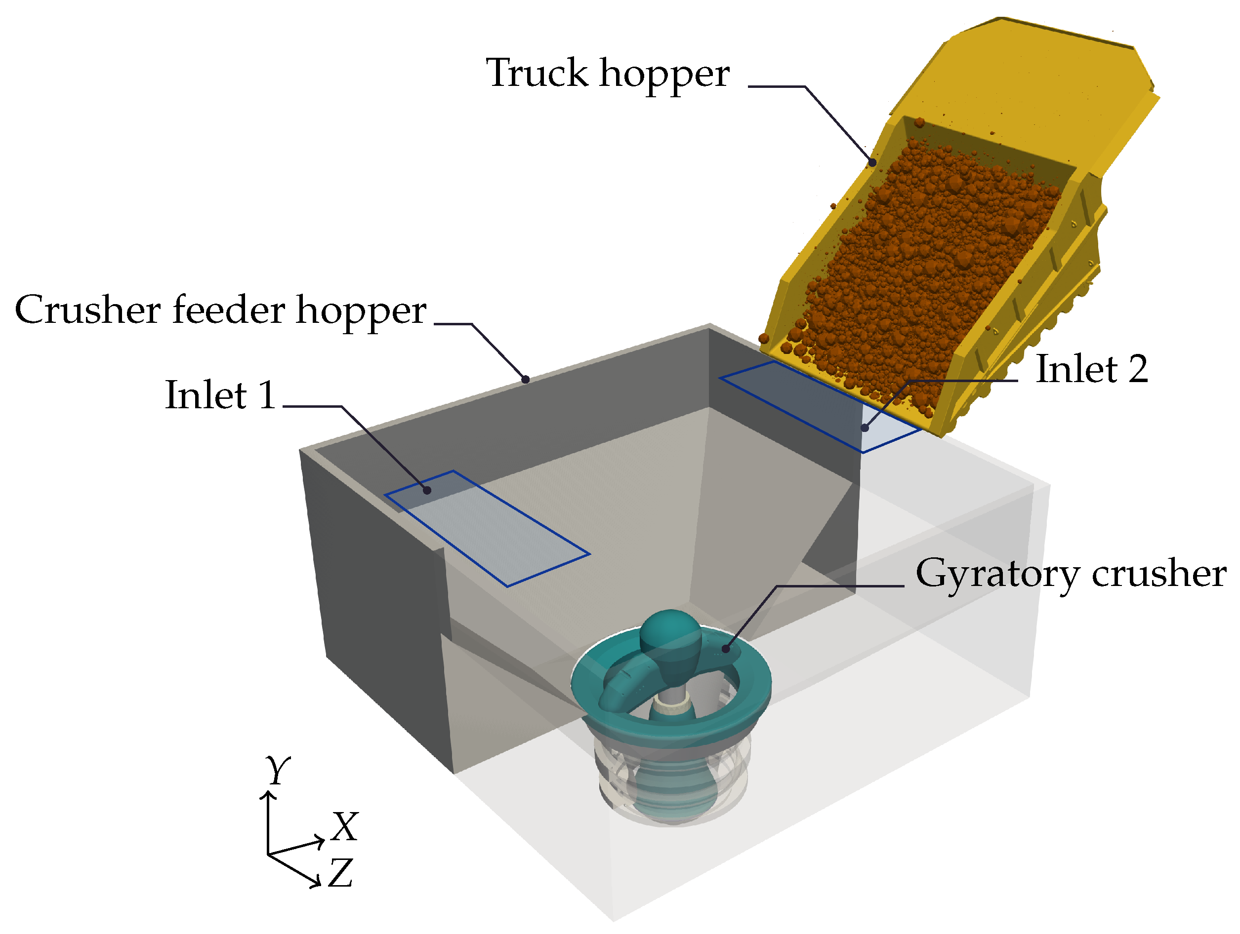
The simulated gyratory crusher is fed by CAT 797F trucks. The nominal capacity of the truck is 293 tons. The truck’s hopper rotates for 15 seconds until it reaches an inclination of 45; then, the mass flow rate of the inlet is 70,320 t/h and the average download speed is 1.8 m/s. To simplify the model, it is possible to set the discharge of the ore by using a rectangular particle inlet per truck with the parameters already mentioned. The most interesting scenario is when two trucks simultaneously feed the crusher; thus, the two inlets are located over the hopper, as is detailed in Figure 5. As the inlet mass flow rate is greater than the expected output mass flow rate, which is between 5000 and 9000 t/h, the crusher will be operating in choke feed conditions.
Simulations are carried out by varying the operating conditions of the crusher, such as the eccentric velocity and the open side setting . To change the , the height of the main shaft was changed in the same manner that it is performed in crushing plants. Four different eccentric rotation speeds and seven different open side settings are contemplated, as is presented in Table 5. The power and throughput obtained in these calculations are compared to the data given by manufacturer specifications for different operating conditions. It is considered a base case, with mm and a of 150 rpm.
The experimental power draw was acquired from current measurement in the electric motor in several charging cycles of the gyratory crusher, operating at rpm and mm. Consequently, the mean no-load power is 443 kW, and the mean crushing power is 1329.4 kW.
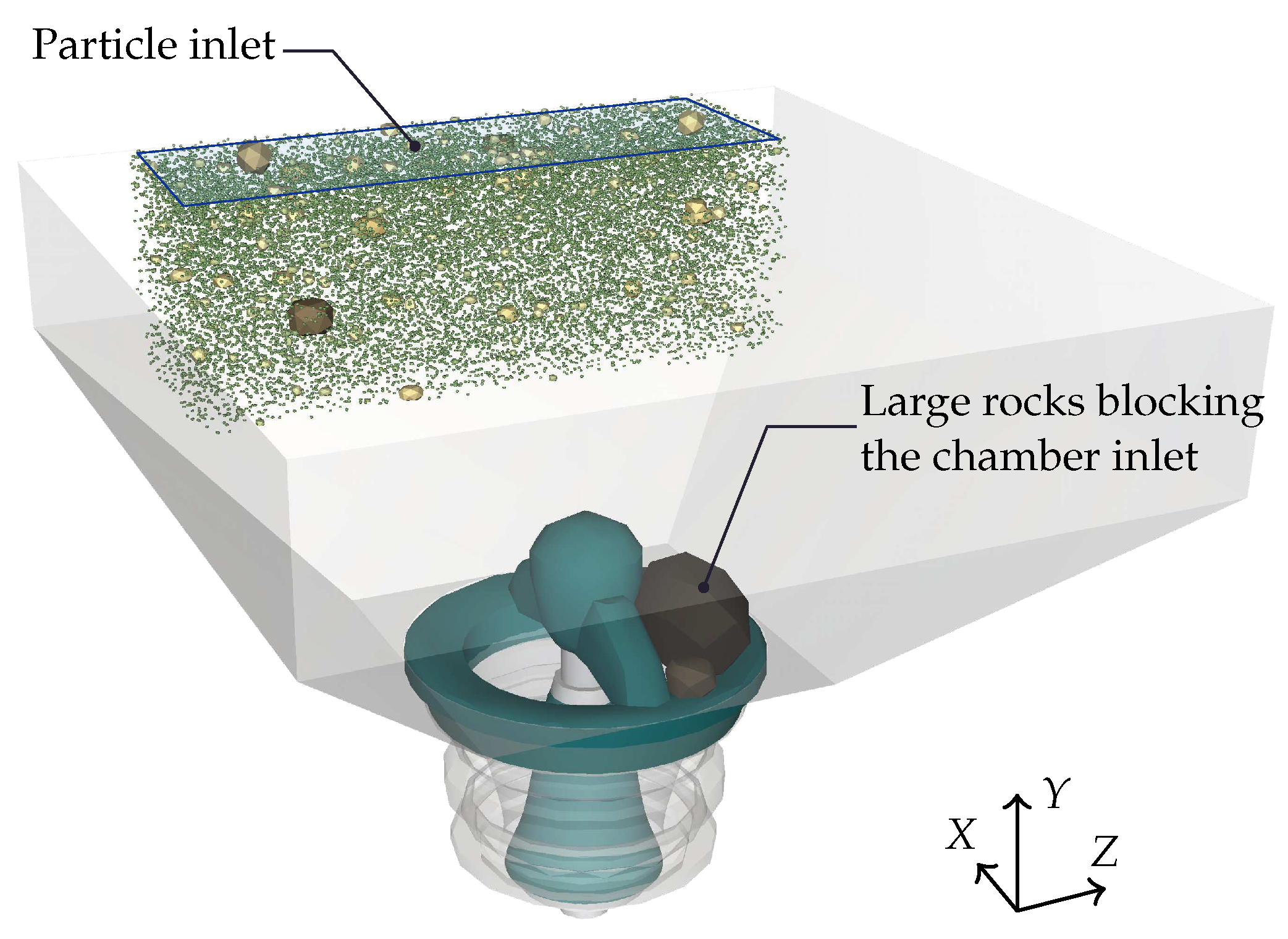
In addition to simulations under ideal conditions, another case is analyzed. The effects of the non-uniform filling (NUF) in the chamber on the crushing torque are studied. One side of the chamber is covered by large rocks between the spider and the top shell. In this way, a region covering 180 of the chamber was fed, as is presented in Figure 6. Only one particle inlet is configured with the same parameters as the previous simulations. This configuration is similar to the one presented in a previous work, where a quarter of a cone crusher was simulated [16].
5. Results
The results of the DEM simulations of the gyratory crusher are presented. It begins with the validation of the model, then the effects of the operational parameters such as and are presented. Finally, the results of the simulation of the non-uniform filling case are shown and compared with the base case.
5.1. Model Validation
Table 6 provides the efficiency and performance of the crusher changing the . The crushing power for mm, base case, is close to the experimental value, 1329.4 kW, and the behavior of the other configurations is as expected. The model correctly predicts the throughput of the crusher because all the mass flow rates of the product calculated in the simulations performed, , are quite close to that indicated by the manufacturer . The error is less than 20% between mm and 200 mm, and the error is less than 10% between 215 mm and 250 mm, which is low compared with the values obtained in the literature [3,16,18]. The product size, represented by the value, is near , as indicated by the manufacturer [43]. As the throughput, product size, and power are close to the ones reported by the manufacturer and the experimental data, the simulation is considered validated.
5.2. Base Case
Figure 7 presents a snapshot of the DEM simulation of the gyratory crusher with mm and rpm, the base case, at simulation time s. At that time, the crushing chamber is full of particles with a total mass of 66,410 kg. In the crushing chamber there are 75,000 particles and there are between 100,000 and 200,000 particles in the entire domain. The median mass flow rate of the product is 8473.0 t/h. At the top of the crusher cavity, the mean particle velocity in the vertical direction is 0.48 m/s, and it is 2.02 m/s at the bottom. As the total particle mass in the chamber and the median mass flow rate of the product remain with low variations, it is considered to be in a steady state.
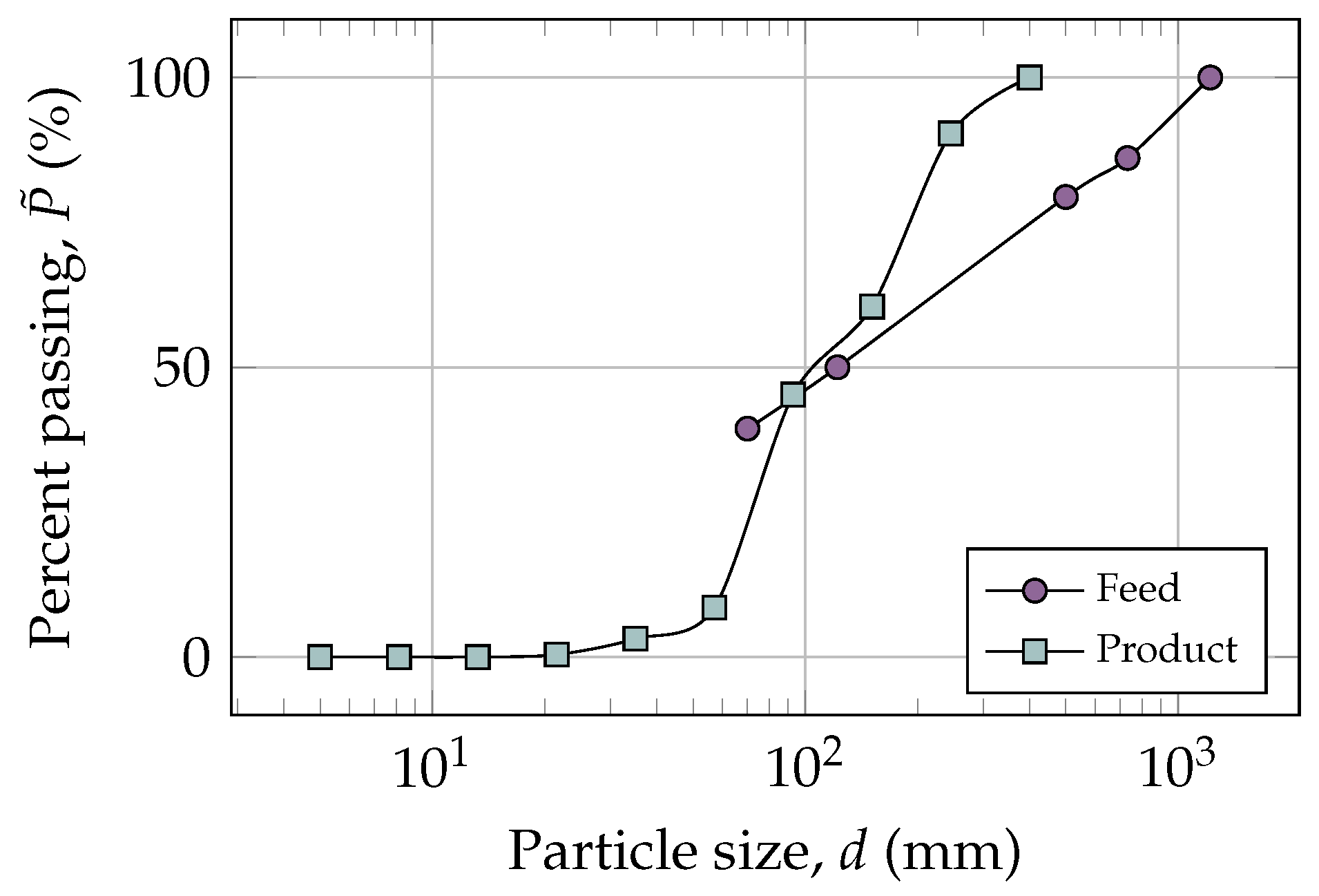
The particle size distribution of the feed and product are exhibited in Figure 8. Comparing the and the feed PSD, more than half of the particles can pass through the crushing chamber without being broken. In the Figure 7, several fine particles with sizes less than 70 mm can be observed in the chamber. For the time s, 8.64% of the mass of fine particles are located in the crusher cavity without been crushed. All the particles of the product have a size less than 400 mm and a equal to 116.43 mm.
The simulated root-mean-square crushing power calculated with all the forces is 1703.3 kW and determined when the torque of the radial forces is 1430.8 kW. Both values of power are quite close to the measured crushing power, with an error of 28.1% and 7.6%, respectively. As was mentioned earlier, this difference is due to the work performed by the transverse forces. The RMS crushing torque is 91.25 kNm.
A complete force distribution analysis acting on the crusher’s mantle is performed. The force profile is exported from Rocky DEM to MATLAB (version R2021a provided by MathWorks, Natick, MA, USA) and Paraview (version 5.9.0 provided by Kitware Inc., Clifton Park, NY, USA). With these post-processing software, it is studied the spatial force distribution over the mantle and the generated torque.
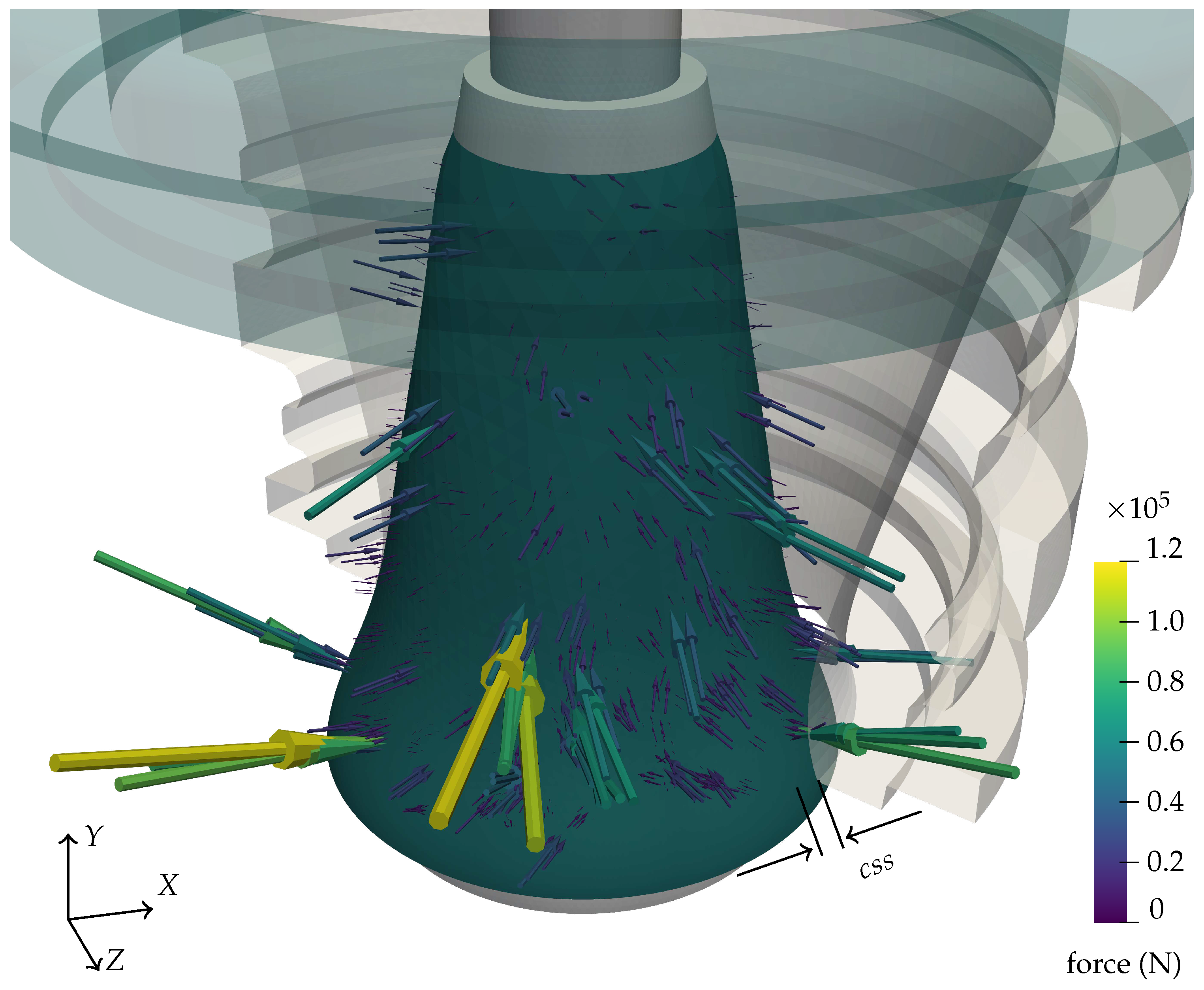
Figure 9 illustrates an example of the prediction of forces on the mantle of the gyratory crusher with the DEM simulation in steady state. Each vector represents the nodal force in the mantle for the given time step. Half of the concave is shown, the hidden part of the concave corresponds to the section where the compression is carried out. The location of the distance is also drawn. As the main shaft rotates in the negative Y direction, the position of the moves in the same direction. The forces cover a surface of half of the mantle (where the concave is hidden) and increase its magnitude when the mantle approaches the concave. A particle–boundary contact can generate more of one nodal force depending on the geometry of the contact, and that is why the nodal forces can be observed to be grouped together.
High magnitude compression forces are presented due to individual compression events. These forces can generate peaks in the power, as it can be observed, both in numerical results [18] and experiments [44].
For the purpose of achieve a representative force distribution that is comparable in different time steps, a moving frame of reference in polar coordinates relative to main shaft is used, as described in Section 2. A planar force distribution in polar coordinates can be obtained, and all the mantle surface can be analyzed in a simple surface plot instead of a 3D graphical representation. This type of graphics can be extracted in all DEM software in terms of normal or shear stress [15], but it is not good for calculating power in the gyratory crusher because only radial forces must be considered in power and torque calculations.
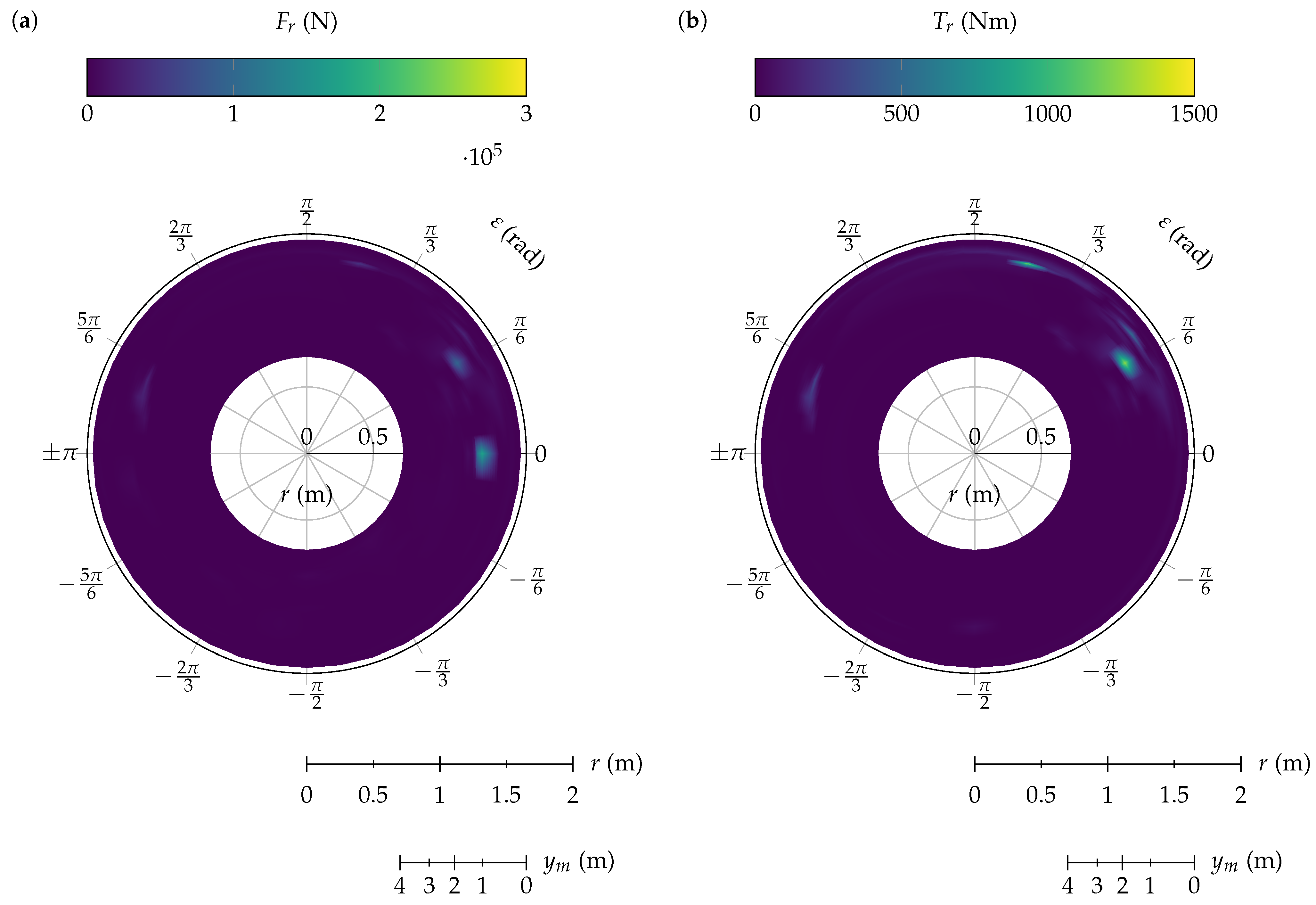
In Figure 10a, the force distribution in polar coordinates of the base case is illustrated. The angle was previously defined and represented the relative position of a node’s mantle regarding the position. The radial coordinate, r, of this polar plot is the radius of the mantle. Additionally, to locate any point in a vertical position of the mantle, a scale of the vertical coordinate, , is added. Both scales are displayed at the bottom. The relationship between r and is the mantle profile shown in Figure 1 and as is not linear, the scale of is non-linear. In this plot, the lower mantle diameter is at the base of the mantle m, and the upper mantle diameter, m, is at the top m. The center of this polar plot corresponds to the geometrical center of the mantle, point . The positive direction of the radial forces is defined by the opposite direction of the unit radial vector, , presented in Figure 2. Since only compression forces were applied over the particles and since there was no adhesion force, all the vectorial components of the forces calculated in these simulations were greater than zero. The radial force distribution is principally concentrated between rad and rad, where the mantle is approaching to concave.
With this force distribution, the crushing torque is determined with Equations (2) and (3). This torque is evaluated regarding the center of the eccentric, located to the left of the center of this polar plot. The positive direction of the torque is defined in the opposite direction of the vertical axis Y coming out of the plane of the graph. Then, the positive radial forces between 0 and produce positive torque, and they produce negative torque between 0 and .
In the torque plot shown in Figure 10b, as it was mentioned before, a drastic change in the value can be observed at rad. The positive torque is principally present between and to where the torque is negative. Between and 0, the mantle moves away from the concave; thus, the forces presented are particles that are in decompression. These forces that produce negative torque are acting for a short period of time.
Comparing the radial force and torque distribution, it can be observed that the torque value depends on the magnitude of the radial force, the vertical position, and the angular position. The lower values of , the greater the eccentricity; therefore, the greater the moment arm will be. For values close to , the moment arm is negligible, and the torque will be close to zero.
5.3. Effect of Open Side Setting
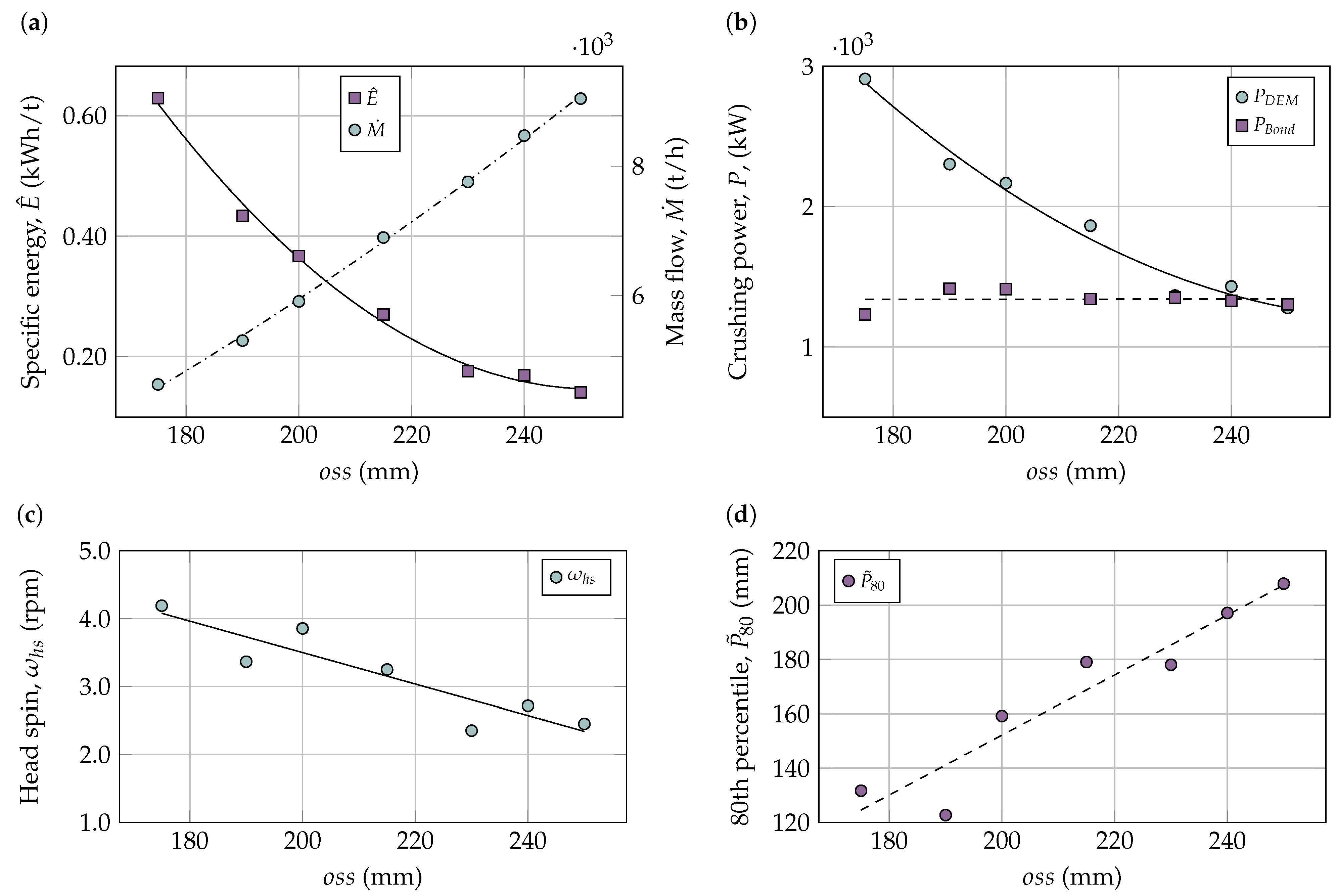
In this subsection, the simulations obtained by changing the are presented. As it is expected, the increase in generates a rise in the discharge mass flow rate due to the flow area is greater. Figure 11a indicates a decrease in the specific energy consumption due to the larger particle size in the discharge, as evidenced by the comparison of the corresponding . This variation in mass flow rate and energy consumption also agrees with data provided by different authors [18,45]. The crushing torque follows the same trend as the crushing power because is fixed.
The PSD of the product is characterized by the , which is illustrated in Figure 11d. All these curves of distribution are similar to the one presented in Figure 8. The is computed with the cumulated product of the crusher in the steady state. The relationship between the and is almost linear, with .
The crushing power computed by DEM with both approaches shown in Table 6 presents a clear difference. Those calculated only with transverse force are less than those calculated with all the forces. Moreover, the calculated with (5) does not have a strict decreasing behavior for equals 200 mm and 240 mm. The power calculated only with radial forces is considered in the following analyses.
A comparison is performed between the power values determined with the discrete element method and those calculated using Bond’s model for different . For Bond’s model, only manufacturer data were used, and the product size was modeled as [43]. The machine parameter, , was fitted to the power of the base case, and the result was 1.286.
Figure 11b shows a comparison between the power evaluated with Bond’s and DEM models. It can be observed that both models can predict the increase in power as the decreases, but the slope in absolute value of the DEM model is significantly greater. Bond’s model is more conservative in calculating power, and the linear fit is almost horizontal, as the difference in power between each is less than 200 kW. The power is almost constant because this model cannot predict high variations. When the changes between 190 mm and 250 mm, the power only changes by 7.9%. On the other hand, in the DEM model for the same change in the , the power varies by 44.5%. Moreover, the power calculated with Bond’s equation for mm is an outlier being the lowest value obtained, and it interrupts the increase in power for mm. These differences can be explained mathematically by the relationship between the throughput that the manufacturer indicates and the . For mm, the difference with the following data is 1410 t/h, and there is a difference of 710 t/h for mm with the previous one, while the other differences remain lesser than 400 t/h.
In Figure 11c, the variation of the head spin regarding the open side setting is presented. The relationship between the head spin and decreases, as it is represented by the linear fit. This behavior can be explained because there are more particles in contact with the mantle when is lower, producing more tangential forces on the mantle. As these results are less than 20 rpm as the manufacturer indicates in no-load conditions, they are considered viable.
5.4. Effect of Eccentric Speed
The effect of the eccentric speed between 100 and 200 rpm on a specific energy consumption is provided in Figure 12a. The specific energy consumption decreased by 55.1% as the eccentric rotation speed decreased by 33.3%. The lowest specific energy consumption was achieved for 100 rpm eccentric speed. This point also increases the mass flow rate in the discharge by 12.8% with respect to the nominal operating conditions and decreases the crushing torque by 26.1%.
The power consumption is highly influenced by the eccentric speed; with an increase in the eccentric rotation speed from 100 to 200 rpm, a 171.4% increase in crushing power was calculated. The torque follows the same tendency, increasing at 35.6% between 100 and 200 rpm.
The mass flow rate in the discharge is maximized when working at 200 rpm. However, it is not recommended to work at this speed since the specific energy consumption increases by 109.1% regarding the 100 rpm simulation.
To choose the rotation speed of the eccentric, it is also important to consider the granulometry in the discharge. Figure 12d presents the 80th percentile of the product size distribution. The complete PSD follows the same trend as the particle size distribution of the base case, shown in Figure 8. The lowest value of was acquired for 150 rpm. On the other hand, by decreasing the rotation speed of the eccentric from 150 to 100 rpm, an increase of 6.91% in the value of was obtained.
A comparison is generated between the power values computed with the discrete element method and those determined by using Bond’s model for different . As the eccentric velocity is not an input parameter of Bond’s model, it is represented by the throughput and product size calculated by DEM simulations. The values utilized here and the resulting findings are presented in the Table 7. Figure 12b presents a comparison between the power evaluated with Bond and the DEM model for different . In these results, Bond’s model is also more conservative. According to the DEM model, doubling the rotational speed of the main shaft increases the power by 271.4%, while the equation of Bond only yielded an increase of 29.3%.
In Figure 12c, the variation of the head spin about the angular speed of the eccentric is plotted. The higher the rotation speed of the eccentric, the higher the head spin, achieving a value of 4.25 rpm at 200 rpm of the eccentric. As the head spin is related to the tangential forces over the mantle with higher , the relative velocities of the mantle and particles are greater and so are the tangential forces. Moreover, more particles are flowing through the crushing chamber, generating more interactions with the mantle. As the particles are moving faster, there are more interactions with the mantle. The linear fit is . In the same manner as the previous results, they are considered viable as they are less than 20 rpm.
5.5. Effect of Non-Uniform Feeding
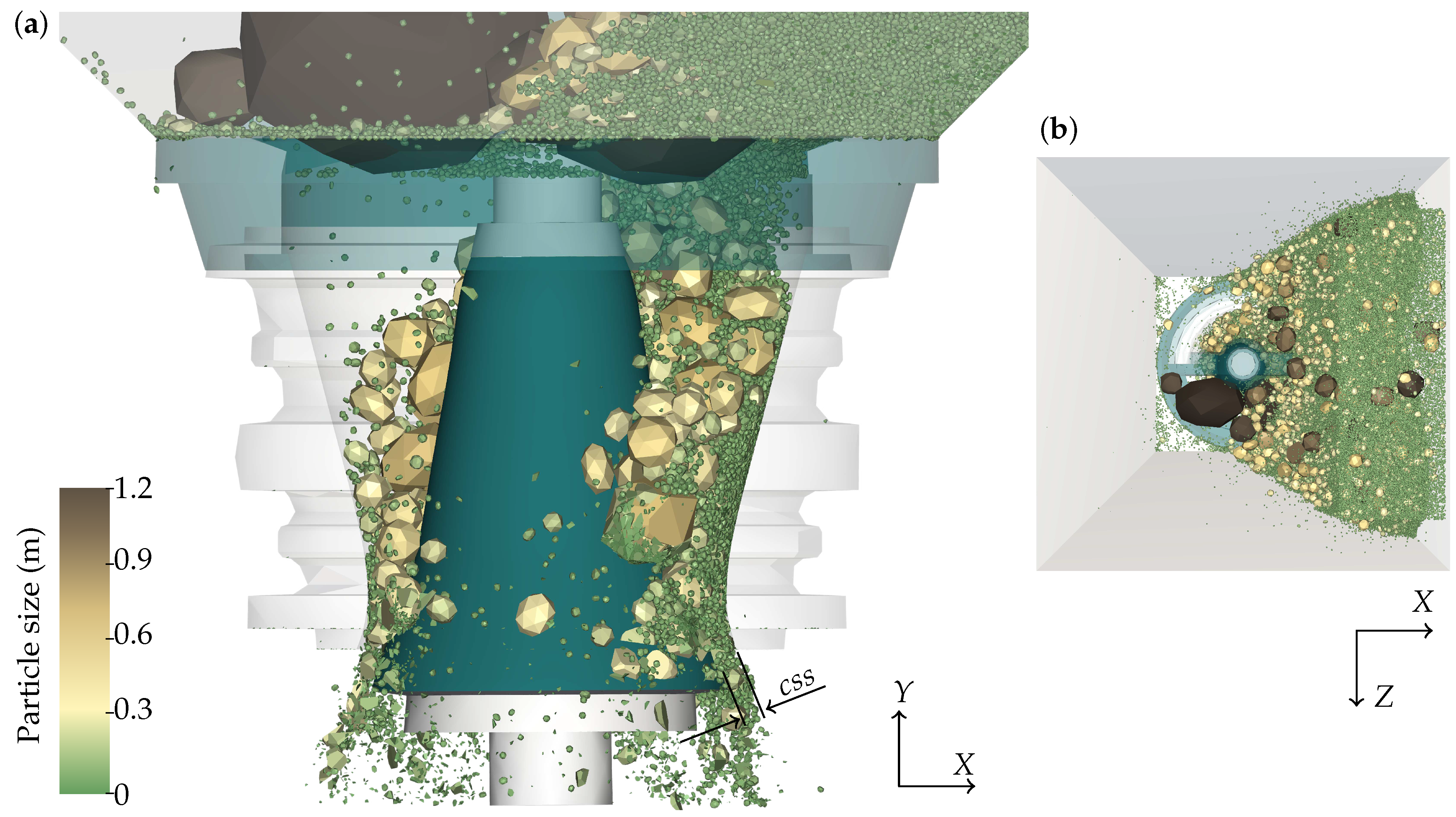
Figure 13 presents an image of the distribution of the particles for the simulation of non-uniform feeding. The truck feeds the crusher from the right side, as can be observed for the concentration of the particles in the top-right corner and in the top view in Figure 13b. Large rocks are in one input of the crusher (the input in the positive z-axis) while the side of the negative Z-axis has an unobstructed entrance, and the particles pass through the right side into the crushing chamber. As the simulation progresses, the left side of the chamber becomes partially filled.
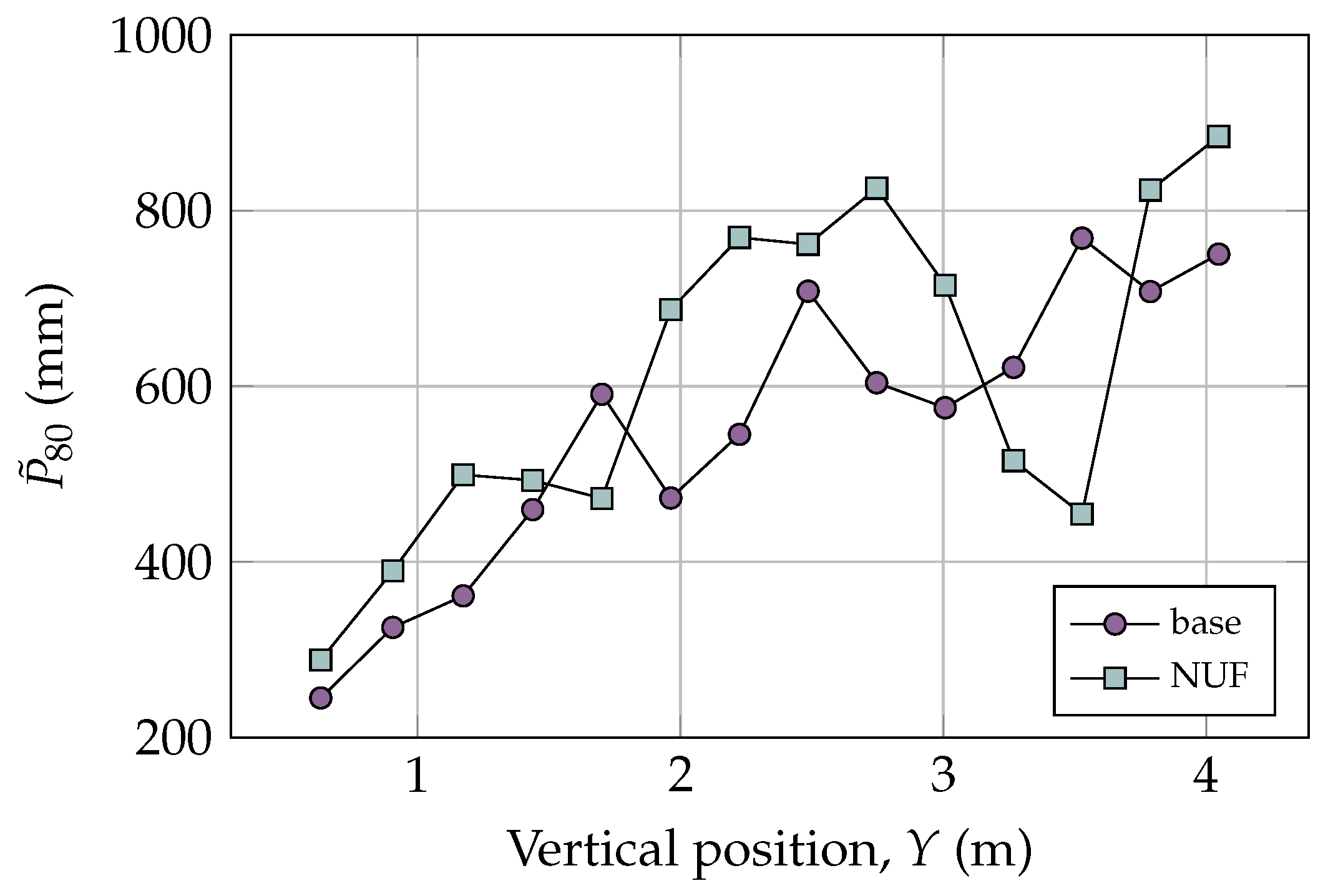
As the particles have greater freedom to move within the chamber, it can be observed that larger particles reach lower areas of the chamber, as it is illustrated in Figure 7 and Figure 13a. To clarify this statement, the is calculated for different vertical positions, Y, of the crushing chamber and is exposed in Figure 14. In general, the non-uniform feeding simulation has greater than the base simulation. This can produce greater torque because, in a lower position, the mantle’s eccentricity is greater. For example, the are 245.0 mm and 288.3 mm for m for the base and non-uniform feeding simulation, respectively. The difference in size is 18% with respect to the base case. If we determine the maximum torque that both particle sizes can produce at that height by using mm, the difference in torque will be 38%.
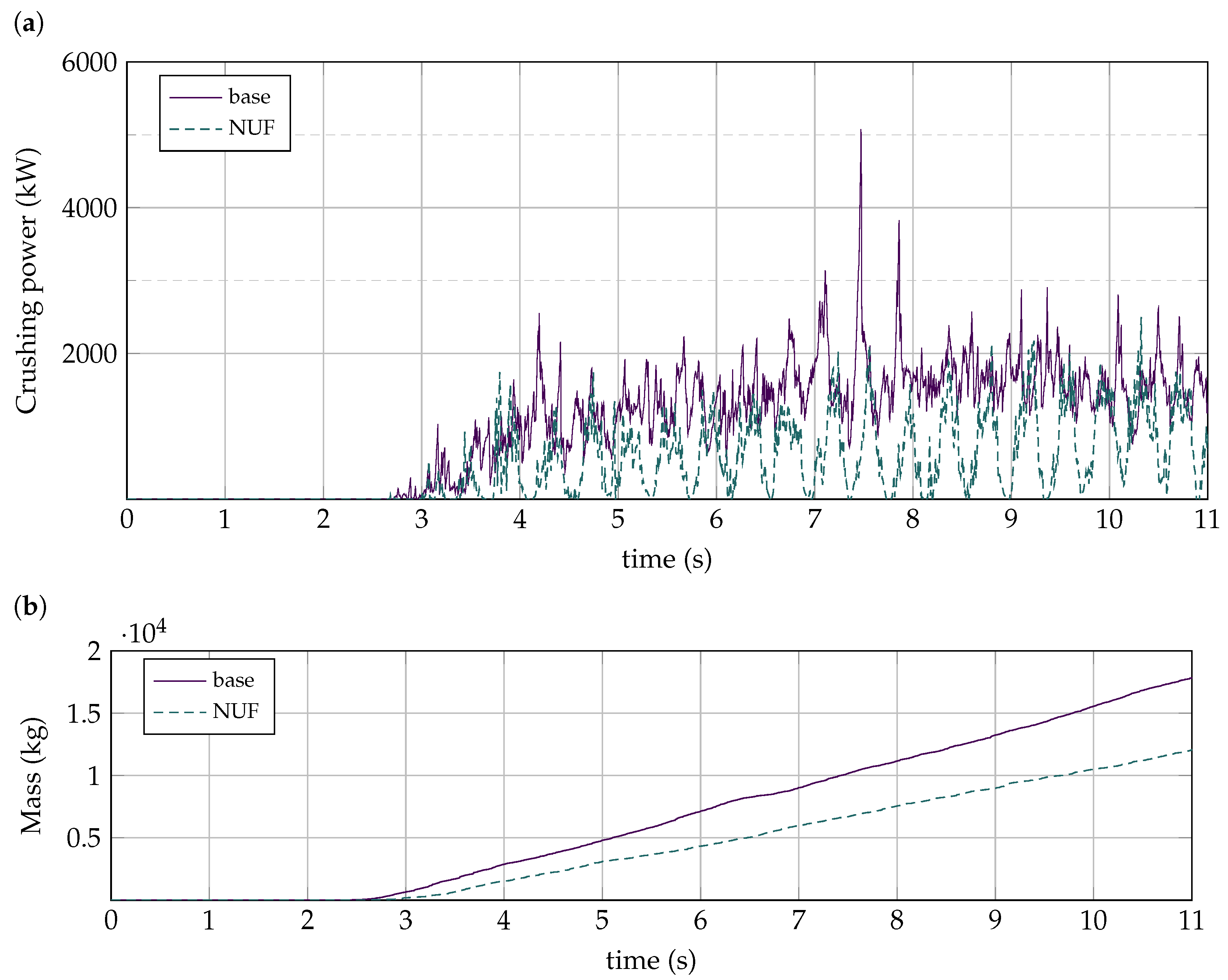
The unbalance of particles in the chamber will affect the power consumption. In Figure 15a, the crushing powers of the non-uniform filling simulation and the base simulation are presented. As the crushing chamber is not perfectly filled, the crushing power of the non-uniform filling simulation shows cycles of loading and unloading with frequency 2.5 Hz, one per revolution, due to the ore being on one side of the crusher cavity. It is expected that the power shows these oscillations, and it does not represent an issue in the machine. When the base case reaches its steady state and the chamber is full of particles, the non-uniform feeding simulation has only one-third of the chamber full at about 9 s, with the total particle mass equal to 22,500 kg. However, both simulations can reach an instantaneous crushing power of 2000 kW. The variance in the crushing power in the base simulation is 0.113 MW, meanwhile, the variance is 0.291 MW in the non-uniform filling simulation.
In these conditions and in some time steps, NUF power peaks are found to be greater than when the chamber is fed uniformly. The mean value of the NUF peaks is 2005 kW, and some valley values of the base case are lower than 1000 kW. This behavior is not expected because the chamber of the base case is full of particles; therefore, the power should be close to the peaks values of the NUF case at all times. This difference in power is because some particles generate negative torque on the mantle when the crushing chamber is full of particles, decreasing the torque value in comparison with the NUF condition.
In the Table 8, a comparison between the base and the non-uniform feeding simulation is carried out. This comparison aims to contrast both simulations when the base case is in steady state starting from 9 s, and the non-uniform filling case is still filling up at this point. If we use data for s, the base case has more particles than the non-uniform filling case, and hence the power is greater. On the other hand, if we utilize , the non-uniform case will be full of particles and both simulations will be almost the same.
Table 8 reports the power draw of both simulations, calculated by adding the no-load power to the crushing power. According to the ones presented in Figure 15a, the power draw in the base case is greater than the non-uniform filling case, principally because it has more particles in contact with the mantle. For the same reason, the throughput is greater in the base case. This throughput is calculated with the cumulative particle mass of the product plotted in Figure 15b. However, the specific energy is less in the base case; thus, the non-uniform filling case requires more energy to process the same mass of ore. The particle size distribution of the product is affected, the of the NUF case is coarser than the base case. This can be compared with non-choke feed conditions, where the particles have greater freedom of movement. Under these conditions, coarser particles were found experimentally in the product [46]. On the other hand, the head spin increases to more than double in the non-uniform feeding case. This is due to there being an imbalance of tangential forces that allows free rotation of the main shaft.
If we extrapolate the data to the complete process, i.e., the crusher fed by two trucks with 293 tons of copper ore in each one, the total crushing time and energy consumption can be determined. The non-uniform filling case takes twice the time and the energy consumption is 23% greater, as it is summarized in Table 8.
In Figure 16, the polar distributions of force and torque are presented. Compared to the base case, it can be observed that zones with non-zero forces are smaller due to the lower number of particles in contact. In Figure 10, it can be observed that there are forces that perform negative torque; meanwhile, the same cannot be detected in the non-uniform feeding case. This brings about an increment in the crushing power, which is shown in Figure 15a, where the non-uniform feeding case with fewer particles can achieve almost the same value of power.
In Figure 16b it is possible to observe that the particles generate torque principally in the first 180 of the mantle. In , there is a zone with force greater than zero in Figure 16a, but the torque is null in Figure 16b. As the moment arm is null, there will be no torque. Furthermore, when the forces are close to , the torque is greater, as can be noticed in the torque between and .
6. Conclusions
- A Metso 60-110 gyratory crusher has been modeled by using the Discrete Element Method with the software Rocky DEM. The diverse comparisons studied clarified that the developed model correctly predicts the performance of the gyratory crusher. The validation was performed in terms of throughput, product size, and crushing power. Nevertheless, there is a lack of availability of complete data sets of crushers due to the challenges related to instrumenting and the very high cost; thus, it is still necessary to validate with data of different crushers in several operational conditions [20].
- It was discussed that the crushing power obtained from torque produced by radial nodal forces is different from the power calculated with all the forces. This difference is because the work of the transverse forces is considered, overestimating the power by approximately 20 percent. This difference is due to the type of movement of the gyratory crusher; thus, using (4) in order to evaluate crushing power in cone crushers is also recommended.
- The proposed change of variable is a suitable tool for analyzing the behavior of loading forces distribution on the mantle. This change of coordinates permits studying the crushing behavior under different operating conditions.
- Regarding the comparison between Bond’s model and the DEM model, both can accurately predict the crushing power. The model of Bond, which is widely used in mining, is more conservative when calculating power under different operating conditions. As it is only an equation, it is convenient for preliminary calculations. For design, optimization, and power analysis in gyratory crushers, it is recommendable to utilize a DEM model, which allows simulations with a high level of detail and under different operating conditions and diverse configurations.
- Under the ideal simulated conditions, the head spin is less than 10% of the rotational speed of the eccentric. As is an ideal case, the presented values of head spin are the lower limit of the head spin and are only produced by the forces of the particles and do not represent a problem or failure in the machine.
- It is recommendable to operate the gyratory crusher with the full crushing chamber, since the following is the case:
- Larger particles are crushing at a higher vertical position that produces lower torque;
- The power and torque have less temporal variation in comparison to the non-uniform case where the crushing power changes from 0 to 2000 kW; avoiding these cycles of load and unload will reduce the fatigue in the machine elements of the gyratory crusher;
- If the crusher is non-uniformly fed, its efficiency can be considerably reduced. The throughput decrease 34% while the total energy consumption increases 20% regarding the ideal case.
- The definition of the ratio of the minimum simulated size will help to configure DEM simulation of crushers. This relationship is focused on the product size, which is essential in crushers.
Author Contributions
Conceptualization, M.M., P.T., F.B. and C.G.R.; methodology, M.M.; software, M.M. and P.T.; validation, M.M., P.T., F.B. and C.G.R.; formal analysis, F.B. and C.G.R.; investigation, M.M.; resources, F.B. and C.G.R.; data curation, M.M.; writing—original draft preparation, M.M., P.T., F.B. and C.G.R.; writing—review and editing, M.M., P.T. and F.B.; visualization, M.M.; supervision, F.B.; project administration, F.B. and C.G.R.; funding acquisition, M.M., F.B. and C.G.R. All authors have read and agreed to the published version of the manuscript.
Funding
M. Moncada acknowledges the funding by the National Agency for Research and Development (ANID) Doctorado Nacional 2019-21192275. F. Betancourt acknowledges the support provided by ANID/FONDAP/15130015 and ANID/PIA/AFB170001.
Data Availability Statement
Not applicable.
Acknowledgments
We acknowledge the ESSS Group S.A. for the research license for this project within the framework of the strategic linkage with the Department of Mechanical Engineering of the University of Concepción. Powered@SouthernGPU: This research was partially supported by the supercomputing infrastructure of the Southern GPU Cluster-Fondequip EQM150134.
Conflicts of Interest
The authors declare no conflict of interest.
Abbreviations
The following abbreviations are used in this manuscript:
| Symbol | Definition |
| BPM | Bonded particle model |
| DEM | Discrete element method |
| NUF | Non-uniform filling |
| PBM | Population balance model |
| PRM | Particle replacement method |
| PSD | Particle size distribution |
| ROM | Run-of-mine |
| Variables | |
| constant parameter | |
| constant parameter | |
| F | force (N) |
| r | position |
| v | velocity |
| ê | unit vector |
| tilt angle () | |
| Ê | Specific energy (kWh/t) |
| stabilization parameter | |
| friction coefficient | |
| angular speed (rad/s) | |
| diameter (m) | |
| angle (rad) | |
| variance | |
| angular position (rad) | |
| constant parameter | |
| amage accumulation coefficient | |
| restitution coefficient | |
| percentile of the feed size distribution (mm) | |
| percentile of the product size distribution (mm) | |
| angle (rad) | |
| constant parameter | |
| A | geometric point |
| b’ | constant parameter |
| css | closed side setting (mm) |
| D | damage |
| E | energy (J) |
| e | eccentricity (mm) |
| H | height (m) |
| K | stiffness (N/m) |
| k | constant parameter or ratio |
| M | mass (kg) |
| O | geometric point |
| O’ | geometric point |
| oss | open side setting (mm) |
| P | power (kW) |
| Q | geometric point |
| r | radius or radial coordinate (m) |
| s | overlap (m) |
| T | torque (Nm) |
| t | time (s) |
| W | work (W) |
| Subindex | |
| normal | |
| max | maximum |
| min | minimum |
| tangential | |
| transverse | |
| c | concave |
| d | kinetic |
| hs | head spin |
| i | index |
| l | loading |
| lo | lower |
| m | machine |
| ms | minimum simulated size |
| mt | mantle |
| p | particle |
| r | radial |
| ref | reference |
| s | static |
| sim | simulated |
| u | unloading |
| up | upper |
| w | wall |
| x | related to x-axis |
| Y | vertical |
| z | related to z-axis |
| 50 | 50th percentile |
| 80 | 80th percentile |
Appendix A. DEM
The following equations are used in the contact and breakage model [34].
Appendix A.1. Contact Model
Normal stiffness between particle i and boundary or particle j as follows:
where is the restitution coefficient. The normal stiffness of a particle o boundary i is as follows:
where d is the particle size. The tangential stiffness is described as follows:
with a constant parameter.
Appendix A.2. Breakage Model
The breakage probability is based on an upper-truncated log-normal distribution of the specific fracture energy. This distribution is defined by the following expression [47].
The relative specific fracture energy is defined as follows:
The relationship between particle size and median fracture energy is described by the following equation.
If the first contact does not generate breakage, the particles will accumulate damage, and the fracture energy will be determined with the following damage model [47].
For each collision event without breakage, the particle accumulated damage; consequently, the new particle-specific fracture energy must be calculated. The damage, D, is given by the following:
where is the damage accumulation coefficient. The size of the progeny of a breakage event is calculated with the percentage in weight of the parent particle that passes through a sieve with an aperture of 10% of the original particle size [47]:
where and are model parameters. The complete particle size distribution is model with an incomplete beta function.
The variable is the percentage of fragments passing a screen size of 1/nth of the original size d. and are model parameters fitted to the experimental data.
References
- Mosher, J. Crushing, Milling, and grinding. In SME Mining Enginering Handbook; Society for Mining, Metallurgy, and Exploration, Inc.: Englewood, CO, USA, 2011; pp. 1461–1480. [Google Scholar]
- de Solminihac, H.; Gonzales, L.E.; Cerda, R. Copper mining productivity: Lessons from Chile. J. Policy Model. 2018, 40, 182–193. [Google Scholar] [CrossRef]
- Johansson, M.; Quist, J.; Evertsson, M.; Hulthén, E. Cone crusher performance evaluation using DEM simulations and laboratory experiments for model validation. Miner. Eng. 2017, 103–104, 93–101. [Google Scholar] [CrossRef]
- Bearman, R.A.; Barley, R.W.; Hitchcock, A. Prediction of power consumption and product size in cone crushing. Miner. Eng. 1991, 4, 1243–1256. [Google Scholar] [CrossRef]
- Liu, R.; Shi, B.; Li, G.; Yu, H. Influence of Operating Conditions and Crushing Chamber on Energy Consumption of Cone Crusher. Energies 2018, 11, 1102. [Google Scholar] [CrossRef] [Green Version]
- Evertsson, M. Modelling of flow in cone crushers. Miner. Eng. 1999, 12, 1479–1499. [Google Scholar] [CrossRef]
- Cundall, P.A.; Strack, O.D.L. A discrete numerical model for granular assemblies. Géotechnique 1979, 29, 47–65. [Google Scholar] [CrossRef]
- Cundall, P.A. A Computer Model for Simulating Progressive, Large-scale Movement in Blocky Rock System. In Proceedings of the International Symposium on Rock Mechanics, Nancy, France, 4–6 October 1971. [Google Scholar]
- Cundall, P. Formulation of a three-dimensional distinct element model—Part I. A scheme to detect and represent contacts in a system composed of many polyhedral blocks. Int. J. Rock Mech. Min. Sci. Geomech. Abstr. 1988, 25, 107–116. [Google Scholar] [CrossRef]
- Hart, R.; Cundall, P.; Lemos, J. Formulation of a three-dimensional distinct element model—Part II. Mechanical calculations for motion and interaction of a system composed of many polyhedral blocks. Int. J. Rock Mech. Min. Sci. Geomech. Abstr. 1988, 25, 117–125. [Google Scholar] [CrossRef]
- Weerasekara, N.; Powell, M.; Cleary, P.; Tavares, L.; Evertsson, M.; Morrison, R.; Quist, J.; Carvalho, R. The contribution of DEM to the science of comminution. Powder Technol. 2013, 248, 3–24. [Google Scholar] [CrossRef]
- Zhu, H.; Zhou, Z.; Yang, R.; Yu, A. Discrete particle simulation of particulate systems: A review of major applications and findings. Chem. Eng. Sci. 2008, 63, 5728–5770. [Google Scholar] [CrossRef]
- Lichter, J.; Lim, K.; Potapov, A.; Kaja, D. New developments in cone crusher performance optimization. Miner. Eng. 2009, 22, 613–617. [Google Scholar] [CrossRef]
- Li, H.; McDowell, G.; Lowndes, I. Discrete element modelling of a rock cone crusher. Powder Technol. 2014, 263, 151–158. [Google Scholar] [CrossRef] [Green Version]
- Delaney, G.; Morrison, R.; Cummins, S.; Cleary, P. DEM modelling of non-spherical particle breakage and flow in an industrial scale cone crusher. Miner. Eng. 2015, 74, 112–122. [Google Scholar] [CrossRef]
- Quist, J.; Evertsson, C.M. Cone crusher modelling and simulation using DEM. Miner. Eng. 2016, 85, 92–105. [Google Scholar] [CrossRef]
- Chen, Z.; Wang, G.; Xue, D.; Bi, Q. Simulation and optimization of gyratory crusher performance based on the discrete element method. Powder Technol. 2020, 376, 93–103. [Google Scholar] [CrossRef]
- André, F.P.; Tavares, L.M. Simulating a laboratory-scale cone crusher in DEM using polyhedral particles. Powder Technol. 2020, 372, 362–371. [Google Scholar] [CrossRef]
- Cheng, J.; Ren, T.; Zhang, Z.; Liu, D.; Jin, X. A Dynamic Model of Inertia Cone Crusher Using the Discrete Element Method and Multi-Body Dynamics Coupling. Minerals 2020, 10, 862. [Google Scholar] [CrossRef]
- Cleary, P.W.; Delaney, G.W.; Sinnott, M.D.; Cummins, S.J.; Morrison, R.D. Advanced comminution modelling: Part 1—Crushers. Appl. Math. Model. 2020, 88, 238–265. [Google Scholar] [CrossRef]
- Chen, Z.; Wang, G.; Xue, D.; Cui, D. Simulation and optimization of crushing chamber of gyratory crusher based on the DEM and GA. Powder Technol. 2021, 384, 36–50. [Google Scholar] [CrossRef]
- Wu, F.; Ma, L.; Zhao, G.; Wang, Z. Chamber Optimization for Comprehensive Improvement of Cone Crusher Productivity and Product Quality. Math. Probl. Eng. 2021, 2021, 5516813. [Google Scholar] [CrossRef]
- Tavares, L.M.; André, F.P.; Potapov, A.; Maliska, C. Adapting a breakage model to discrete elements using polyhedral particles. Powder Technol. 2020, 362, 208–220. [Google Scholar] [CrossRef]
- Barrios, G.K.; Jiménez-Herrera, N.; Fuentes-Torres, S.N.; Tavares, L.M. DEM Simulation of Laboratory-Scale Jaw Crushing of a Gold-Bearing Ore Using a Particle Replacement Model. Minerals 2020, 10, 717. [Google Scholar] [CrossRef]
- Wills, B.A.; Finch, J.A. Crushers. In Wills’ Mineral Processing Technology; Elsevier: Amsterdam, The Netherlands, 2016; pp. 123–146. [Google Scholar] [CrossRef]
- Rose, H.E.; English, J.E. Theoretical analysis of the performance of jaw crushers. IMM Trans. 1967, 76, C32. [Google Scholar]
- Pothina, R.; Kecojevic, V.; Klima, M.S.; Komljenovic, D. Gyratory crusher model and impact parameters related to energy consumption. Min. Metall. Explor. 2007, 24, 170–180. [Google Scholar] [CrossRef]
- Pulgar, J.V.; Valenzuela, M.A.; Vicuna, C.M. Correlation between Power and Lifters Forces in Grinding Mills. IEEE Trans. Ind. Appl. 2019, 55, 4417–4427. [Google Scholar] [CrossRef]
- Barrios, G.K.; Tavares, L.M. A preliminary model of high pressure roll grinding using the discrete element method and multi-body dynamics coupling. Int. J. Miner. Process. 2016, 156, 32–42. [Google Scholar] [CrossRef]
- Nagata, Y.; Tsunazawa, Y.; Tsukada, K.; Yaguchi, Y.; Ebisu, Y.; Mitsuhashi, K.; Tokoro, C. Effect of the roll stud diameter on the capacity of a high-pressure grinding roll using the discrete element method. Miner. Eng. 2020, 154, 106412. [Google Scholar] [CrossRef]
- Horváth, D.; Poós, T.; Tamás, K. Modeling the movement of hulled millet in agitated drum dryer with discrete element method. Comput. Electron. Agric. 2019, 162, 254–268. [Google Scholar] [CrossRef]
- Lemieux, M.; Léonard, G.; Doucet, J.; Leclaire, L.A.; Viens, F.; Chaouki, J.; Bertrand, F. Large-scale numerical investigation of solids mixing in a V-blender using the discrete element method. Powder Technol. 2008, 181, 205–216. [Google Scholar] [CrossRef]
- Owen, P.J.; Cleary, P.W. Screw conveyor performance: Comparison of discrete element modelling with laboratory experiments. Prog. Comput. Fluid Dyn. Int. J. 2010, 10, 327. [Google Scholar] [CrossRef]
- ESSS. DEM Technical Manual 4.2; ESSS: Florianópolis, Brazil, 2018. [Google Scholar]
- Imai, H.; Iri, M.; Murota, K. Voronoi Diagram in the Laguerre Geometry and Its Applications. SIAM J. Comput. 1985, 14, 93–105. [Google Scholar] [CrossRef]
- Barrios, G.K.; de Carvalho, R.M.; Tavares, L.M. Modeling breakage of monodispersed particles in unconfined beds. Miner. Eng. 2011, 24, 308–318. [Google Scholar] [CrossRef]
- Cleary, P.W.; Morrison, R.D. Geometric analysis of cone crusher liner shape: Geometric measures, methods for their calculation and linkage to crusher behaviour. Miner. Eng. 2021, 160, 106701. [Google Scholar] [CrossRef]
- Mc Dowell, G.; de Bono, J. On the micro mechanics of one-dimensional normal compression. Géotechnique 2013, 63, 895–908. [Google Scholar] [CrossRef] [Green Version]
- Ciantia, M.; Arroyo, M.; Calvetti, F.; Gens, A. An approach to enhance efficiency of DEM modelling of soils with crushable grains. Géotechnique 2015, 65, 91–110. [Google Scholar] [CrossRef] [Green Version]
- Prabhu, S.; Qiu, T. Modeling of Sand Particle Crushing in Split Hopkinson Pressure Bar Tests using the Discrete Element Method. Int. J. Impact Eng. 2021, 360, 103974. [Google Scholar] [CrossRef]
- Zhou, W.; Wang, D.; Ma, G.; Cao, X.; Hu, C.; Wu, W. Discrete element modeling of particle breakage considering different fragment replacement modes. Powder Technol. 2020, 360, 312–323. [Google Scholar] [CrossRef]
- Cleary, P.W.; Sinnott, M.D.; Morrison, R.D.; Cummins, S.; Delaney, G.W. Analysis of cone crusher performance with changes in material properties and operating conditions using DEM. Miner. Eng. 2017, 100, 49–70. [Google Scholar] [CrossRef]
- Metso:Outotec. Basics in Minerals Processing, 12th ed.; Metso Outotec Corporation: Helsinki, Finland, 2021. [Google Scholar]
- Gröndahl, A.; Asbjörnsson, G.; Hulthén, E.; Evertsson, M. Diagnostics of cone crusher feed segregation using power draw measurements. Miner. Eng. 2018, 127, 15–21. [Google Scholar] [CrossRef]
- Lindqvist, M.; Evertsson, C.M. Improved flow- and pressure model for cone crushers. Miner. Eng. 2004, 17, 1217–1225. [Google Scholar] [CrossRef]
- Ron Simkus, A.D. Tracking hardness and size: Measuring and monitoring ROM ore properties at Highland Valley copper. In Proceedings of the Mine to Mill 1998 Conference, Brisbane, Australia, 11–14 October 1998. [Google Scholar]
- Tavares, L.M. Analysis of particle fracture by repeated stressing as damage accumulation. Powder Technol. 2009, 190, 327–339. [Google Scholar] [CrossRef]
Figure 1.
Metso 60-110 gyratory crusher. Concave cut in half, mantle, main shaft, and spider are presented. Some geometrical parameters are presented, such as the height, ; upper diameter, ; lower diameter of the mantle () and the upper diameter ; and lower diameter of the concave (c). A geometric scale is drawn at the right bottom.

Figure 2.
Geometric parameters of the gyratory crusher, force decomposition, and moving frame of reference. Tilt angle, ; pivot point, Q; eccentricity at the base of the mantle, ; open side setting, ; closed side setting, ; axial axis of the main shaft, ; the fixed and moving frame of reference are presented for the simulation time t such that . A force is applied in point A, showing their radial ; transverse ; and vertical components. The position of A is represented by , , and , and the radial direction is represented by . Both points O and belong to the horizontal plane.

Figure 3.
(a) Mixer with a mobile rectangular plate rotating around the vertical axis. The force is applied at the rectangular plate. (b) Cross-section of the mantle with a vector force, , applied at point A. The node i and all the cross-section has velocity . (c) Rectangular decomposition of the force, , in radial and transverse direction. (d) Rectangular decomposition of the force, , at the x-axis and z-axis.

Figure 4.
Particle shapes: (a) particle 1, (b) particle 2, (c) particle 3, and (d) particle 4.

Figure 5.
Schematic diagram of the primary crusher used in DEM simulation and the complete setup, showing the truck hopper, crusher feeder hopper, and two rectangular inlets.
Figure 5.
Schematic diagram of the primary crusher used in DEM simulation and the complete setup, showing the truck hopper, crusher feeder hopper, and two rectangular inlets.

Figure 6.
Non-uniform filling simulation setup. Large rocks are inserted covering a feed inlet, and one side of the chamber is fed.
Figure 6.
Non-uniform filling simulation setup. Large rocks are inserted covering a feed inlet, and one side of the chamber is fed.

Figure 7.
Snapshot of the base simulation at s showing a frontal section of the crusher. The particles are colored by their particle size, and the concave was cut to observe the particles. The position of the closed side setting, , is also presented.
Figure 7.
Snapshot of the base simulation at s showing a frontal section of the crusher. The particles are colored by their particle size, and the concave was cut to observe the particles. The position of the closed side setting, , is also presented.

Figure 8.
DEM simulated feed and product particle size distributions. The feed is common for all the simulations, and the product is for the base case.
Figure 8.
DEM simulated feed and product particle size distributions. The feed is common for all the simulations, and the product is for the base case.

Figure 9.
Nodal forces at simulation time s. The length and the color of the vector represent the magnitude of the force vectors. The position of the closed side setting, , is also presented.
Figure 9.
Nodal forces at simulation time s. The length and the color of the vector represent the magnitude of the force vectors. The position of the closed side setting, , is also presented.

Figure 10.
Polar distributions of the base case at simulation time s of the base case: (a) radial forces and (b) torque of radial forces. is the transverse direction, r is the radial direction, and is the vertical direction. Each surface plot represents a top view of the mantle.
Figure 10.
Polar distributions of the base case at simulation time s of the base case: (a) radial forces and (b) torque of radial forces. is the transverse direction, r is the radial direction, and is the vertical direction. Each surface plot represents a top view of the mantle.

Figure 11.
Results of simulations changing the open side setting: (a) mass flow rate and specific energy, (b) power comparison with Bond, (c) head spin, and (d) 80th percentile of the product size distribution.
Figure 11.
Results of simulations changing the open side setting: (a) mass flow rate and specific energy, (b) power comparison with Bond, (c) head spin, and (d) 80th percentile of the product size distribution.

Figure 12.
Results of simulations changing the eccentric angular speed: (a) mass flow rate and specific energy, (b) power comparison with Bond, (c) head spin, and (d) 80th percentile of the product size distribution.
Figure 12.
Results of simulations changing the eccentric angular speed: (a) mass flow rate and specific energy, (b) power comparison with Bond, (c) head spin, and (d) 80th percentile of the product size distribution.

Figure 13.
Snapshot of the non-uniform feeding simulation at s showing a frontal section of the crusher. The particles are colored by their particle size, and the concave was cut in order to observe the particles. The position of the closed side setting, , is also presented: (a) frontal view and (b) top view.

Figure 14.
Eightieth percentile of the product size distribution vs. the vertical position of the particles in the crushing chamber.
Figure 14.
Eightieth percentile of the product size distribution vs. the vertical position of the particles in the crushing chamber.

Figure 15.
Comparison between base and non-uniform feeding simulations: (a) crushing power and (b) cumulative mass of the product.
Figure 15.
Comparison between base and non-uniform feeding simulations: (a) crushing power and (b) cumulative mass of the product.

Figure 16.
Polar distributions of the non-uniform feeding case at simulation time s: (a) radial forces, and (b) torque of radial forces. is the transverse direction, r is the radial direction, and is the vertical direction. Each surface plot represent a top view of the mantle.
Figure 16.
Polar distributions of the non-uniform feeding case at simulation time s: (a) radial forces, and (b) torque of radial forces. is the transverse direction, r is the radial direction, and is the vertical direction. Each surface plot represent a top view of the mantle.


Table 1.
Geometrical and material parameters of the geometries of the DEM simulation.
| Variable | Value |
|---|---|
| Length of the crusher feeder hopper (m) | 18.0 |
| Height of the crusher feeder hopper (m) | 9.0 |
| Height of the mantle, (m) | 4.0 |
| Upper mantle diameter, (m) | 1.4 |
| Lower mantle diameter, (m) | 3.3 |
| Upper concave diameter, (m) | 4.9 |
| Lower concave diameter, (m) | 3.5 |
| Eccentricity at the base of the main shaft, (mm) | 46.6 |
| Density (kg/m) | 7800 |
| Inclination, () | 0.35 |
| Main shaft’s mass (kg) | 176,760 |
| Main shaft’s inertia (kg m) | 126,323.4 |
Table 2.
Material parameters of the copper ore [18].
Table 2.
Material parameters of the copper ore [18].
| Variable | Value |
|---|---|
| Inlet mass flow rate (t/h) | 70,320 |
| Number of particles in the crushing chamber | 75,000 |
| Particle shape | Polyhedral |
| Particle size (m) | 1.22, 0.732, 0.5, 0.122, 0.07 |
| Cumulative particle size distribution (%) | 100, 86.1, 79.39, 50, 39.42 |
| Density (kg/m) | 2930 |
| Restitution coefficient | 0.3 |
| Static friction coefficient, ; | 0.8; 0.5 |
| Dynamic friction coefficient, ; | 0.8; 0.5 |
Table 3.
Breakage parameters of the copper ore [18].
Table 3.
Breakage parameters of the copper ore [18].
| Variable | Value |
|---|---|
| (J/kg) | 213.5 |
| (mm) | 8.07 |
| 1.22 | |
| 0.799 | |
| 0.51/11.95 | |
| 1.07/13.87 | |
| 1.01/8.09 | |
| 1.08/3.03 | |
| 1.01/0.53 | |
| 1.03/0.36 | |
| 1.03/0.30 | |
| 5.0 | |
| (%) | 67.7 |
| 0.029 | |
| (mm) | 10 |
Table 4.
Ratio of the minimum simulated size, used in DEM simulations of gyratory and cone crushers.
Table 4.
Ratio of the minimum simulated size, used in DEM simulations of gyratory and cone crushers.
| Reference | (mm) | (mm) | |
|---|---|---|---|
| Litcher et al. [13] | 5 | 1.5 | 3.33 |
| Li et al. [14] | 12 | 4 | 3 |
| Delaney et al. [15] | 11 | 8 | 1.375 |
| Quist et al. [16] | 34 | 4.8 | 7.08 |
| Johansson et al. [3] | 2.2 | 1 | 2.2 |
| Chen et al. [17] | 120 | 30 | 4 |
| Andre et al. [18] | 4 | 1.9 | 2.11 |
| Cleary et al. [20,42] | 11 | 6.7 | 1.64 |
| This paper | 111.62 | 10 | 11.16 |
Table 5.
Operating parameters and simulation conditions.
| Variable | Value |
|---|---|
| Open side setting, (mm) | 175, 190, 200, 215, 230, 240, 250 |
| Closed side setting, (mm) | 111.62, 126.98, 137.23, 152.51, |
| 167.72, 177.90, 188.11 | |
| Angular speed of the eccentric, (rpm) | 100, 125, 150, 175, 200 |
Table 6.
Simulation results at different open side settings and rpm and crushing power calculated with Bond’s equation. The throughput of the manufacturer (ref.) and the simulated ones with DEM (sim.) are presented. The power calculated by DEM with all the forces (5) and only radial forces (4) calculated by Bond’s equation are tabulated.
| (mm) | (t/h) | P (kW) | T (kNm) | (mm) | |||
|---|---|---|---|---|---|---|---|
| ref. | sim. | DEM Equation (5) | DEM Equation (4) | Bond Equation (1) | |||
| 175 | 5535 | 4626.5 | 3464.3 | 2910.0 | 1231.3 | 185.3 | 131.7 |
| 190 | 6945 | 5304.4 | 2378.4 | 2302.7 | 1415.2 | 146.6 | 122.7 |
| 200 | 7335 | 5910.3 | 2573.2 | 2167.4 | 1411.9 | 138.0 | 159.2 |
| 215 | 7570 | 6897.5 | 2212.9 | 1863.9 | 1340.5 | 118.7 | 179.0 |
| 230 | 8280 | 7758.3 | 1619.8 | 1366.0 | 1351.2 | 87.0 | 178.0 |
| 240 | 8595 | 8473.0 | 1703.3 | 1430.8 | 1329.4 | 91.3 | 197.1 |
| 250 | 8890 | 9044.9 | 1512.4 | 1277.5 | 1303.8 | 81.3 | 207.9 |
Table 7.
Simulation results at different eccentric speed and mm and crushing power calculated with Bond’s equation.
Table 7.
Simulation results at different eccentric speed and mm and crushing power calculated with Bond’s equation.
| (rpm) | (t/h) | P (kW) | T (kNm) | (mm) | ||
|---|---|---|---|---|---|---|
| DEM Equation (5) | DEM Equation (4) | Bond Equation (1) | ||||
| 100 | 8079.9 | 947.9 | 804.8 | 1104.1 | 76.9 | 210.7 |
| 125 | 8199.6 | 1316.2 | 1111 | 1183.1 | 84.5 | 202.5 |
| 150 | 8473.0 | 1703.3 | 1430.8 | 1266.8 | 91.254 | 197.1 |
| 175 | 8327.3 | 2229.3 | 1883.6 | 1221.6 | 102.76 | 200.0 |
| 200 | 10,485.0 | 2590.6 | 2187.4 | 1561.5 | 104.3 | 197.7 |
Table 8.
Comparison of results between the base simulation and the non-uniform feeding simulations.
| Variable | Base | Non-Uniform Feeding |
|---|---|---|
| Power draw (kW) | 1979.3 | 1422.1 |
| Throughput, (t/h) | 8473.0 | 5556.6 |
| Specific energy (kWh/t) | 0.2377 | 0.2559 |
| 80th percentile of the product size distribution (mm) | 223.52 | 239.27 |
| Head spin (rpm) | 2.718 | 6.2621 |
| Total crushing time (min) | 4.11 | 6.46 |
| Total energy consumption (kWh) | 0.0377 | 0.0455 |
Publisher’s Note: MDPI stays neutral with regard to jurisdictional claims in published maps and institutional affiliations. |
© 2021 by the authors. Licensee MDPI, Basel, Switzerland. This article is an open access article distributed under the terms and conditions of the Creative Commons Attribution (CC BY) license (https://creativecommons.org/licenses/by/4.0/).
Share and Cite
MDPI and ACS Style
Moncada, M.; Toledo, P.; Betancourt, F.; Rodríguez, C.G. Torque Analysis of a Gyratory Crusher with the Discrete Element Method. Minerals 2021, 11, 878. https://0-doi-org.brum.beds.ac.uk/10.3390/min11080878
AMA Style
Moncada M, Toledo P, Betancourt F, Rodríguez CG. Torque Analysis of a Gyratory Crusher with the Discrete Element Method. Minerals. 2021; 11(8):878. https://0-doi-org.brum.beds.ac.uk/10.3390/min11080878
Chicago/Turabian StyleMoncada, Manuel, Patricio Toledo, Fernando Betancourt, and Cristian G. Rodríguez. 2021. "Torque Analysis of a Gyratory Crusher with the Discrete Element Method" Minerals 11, no. 8: 878. https://0-doi-org.brum.beds.ac.uk/10.3390/min11080878
Note that from the first issue of 2016, this journal uses article numbers instead of page numbers. See further details here.