
Comparison of Semirigorous and Empirical Models Derived Using Data Quality Assessment Methods


1
School of Chemical and Metallurgical Engineering, University of the Witwatersrand, Johannesburg 2000, South Africa
2
Department of Electrical, Electronic and Computer Engineering, University of Pretoria, Pretoria 0002, South Africa
3
Department of Automation Engineering, Technical University of Ilmenau, 99084 Ilmenau, Germany
4
Anglo American, Johannesburg 2000, South Africa
*
Author to whom correspondence should be addressed.
†
These authors contributed equally to this work.
Minerals 2021, 11(9), 954; https://0-doi-org.brum.beds.ac.uk/10.3390/min11090954
Submission received: 28 June 2021
/
Revised: 21 August 2021
/
Accepted: 23 August 2021
/
Published: 31 August 2021
(This article belongs to the Special Issue The Application of Machine Learning in Mineral Processing)
Abstract
:With the increase in available data and the stricter control requirements for mineral processes, the development of automated methods for data processing and model creation are becoming increasingly important. In this paper, the application of data quality assessment methods for the development of semirigorous and empirical models of a primary milling circuit in a platinum concentrator plant is investigated to determine their validity and how best to handle multivariate input data. The data set used consists of both routine operating data and planned step tests. Applying the data quality assessment method to this data set, it was seen that selecting the appropriate subset of variables for multivariate assessment was difficult. However, it was shown that it was possible to identify regions of sufficient value for modeling. Using the identified data, it was possible to fit empirical linear models and a semirigorous nonlinear model. As expected, models obtained from the routine operating data were, in general, worse than those obtained from the planned step tests. However, using the models obtained from routine operating data as the initial seed models for the automated advanced process control methods would be extremely helpful. Therefore, it can be concluded that the data quality assessment method was able to extract and identify regions sufficient and acceptable for modeling.
1. Introduction
As the importance of data increases and increasingly large amounts of data are collected by industrial processes [1,2], there is a growing need to develop methods that can automate the processing of the data. However, much of the data are directly used without any consideration of its quality. The famous computing adage, attributed originally to George Fuechsel, a programming instructor at IBM who used it as a teaching device in the late 1950s [3] goes “garbage in, garbage out”. In the context of modeling, this means that if the data provided are useless, then the resulting analysis will also be useless.
In process control, one of the most important applications of data is for understanding the process, that is, developing models that describe the behaviour of the system for different situations [4]. In process modeling, the key metric for determining the quality of the data is persistent excitation, which measures how much of the system has been excited [5,6]. Traditionally, persistent excitation is used to design experiments so that the maximal amount of information can be extracted from the experiment [6]. Operating companies who are involved in MPC projects often ask the question “why can we not use all the historical data that we have gathered for our process to derive the models”? This is a valid question, and the standard answers are listed below.
- The modes of the PID loops in the past are not known.
- The data are correlated and cannot be used.
- There is too much data to look through to find regions where model identification can be used.
This paper aims to redress these areas using a case study with analysis of real plant data. The short answers to the concerns are below.
- Either store the modes, or calculate them from the setpoint, process value, and output behaviour.
- Modern identification techniques can handle a certain amount of cross-correlation in the data.
- In this era of big data, can we not write a routine that partitions the data for us?
With the growth of data-driven methods, it is now necessary to test the available data to determine if it satisfies this condition. This approach is often called data quality assessment (DQA) [7,8,9]. DQA consists of three main steps: preprocessing, assessment, and postprocessing. In the preprocessing step, any known process changes are used to partition the data set into known regions, while the assessment step takes each of the known regions and seeks to determine which segments are sufficiently exciting. Finally, the segments are analyzed to determine if any of them are similar in nature and could be considered to come from a single underlying region. The need for postprocessing arises from two constraints: First, the assessment method can be a bit too conservative and split adjacent data sets into multiple segments even if they come from the same underlying model. Second, within the original data set, there may be multiple instances of the same model. Combining these regions has the advantage of increasing the amount of available data so that better models can be obtained. Another large issue in DQA is how to handle multivariate data sets, where some, but not necessarily all, of the input variables are needed for modeling the process [10]. Clearly, if all the redundant data are used, then the data quality will automatically be assessed as being bad, as the information matrix will be uninvertible. However, there may well be a subset of inputs that can in fact be used to model the data set. Therefore, there is a need to determine which subset can or should be used to model the data set.
Another critical aspect for DQA that has not been well studied is the development of methods that can be applied to the modeling of different types of models. Most DQA methods focus on data-driven, black-box models. However, other types of models can also be created, such as semirigorous, gray-box models, where the overall form of the model is developed from a theoretical understanding of the model, but whose parameter values are determined based on the available data. A comparison of the applicability of DQA for such models would also be helpful.
Therefore, this paper will examine the problem of DQA for multivariate data sets and its application to both data-driven and semirigorous models. The results will be shown using data taken from the primary milling circuit in a platinum concentrator plant.
2. Data Quality Assessment Method
DQA seeks to extract from a historical data set those regions that are of interest for the engineer or user. In such cases, the important factor is identifiability or whether the particular data set can be used for modeling the process. Clearly, a variable whose value does not change is not effective for modeling the process. In general, identifiability is linked with the invertibility of the Fisher information matrix, which measures the amount of information present in the input signals about the parameters of interest [11]. However, in practical terms, other factors, such as the variance of the signals and missing data, need to also be considered [12].
Furthermore, extending the results to the multivariate case requires that additional factors be considered. From the perspective of invertibility of the Fisher information matrix, collinearity of the variables is an important factor to avoid. This means that within a given historical data set some of the variables may be correlated with each other. Placing both of these variables into the Fisher information matrix will cause the matrix to be uninvertible, and thus the data region will be considered useless. One easy solution to this problem is to examine the correlations between the variables and only select those that are not correlated with each other. A further area of concern is that such variables may also be correlated as a function of a delay. This will complicate the problem even further and make searching for an uncorrelated set more difficult.
Multivariate Data Segmentation Algorithm
In order to consider multivariate data segmentation, the following changes need to be made to the overall data segmentation algorithm:
- Preprocessing: The data set is first loaded and preprocessed. Often preprocessing consists of scaling and centering the data.
- Mode Changes: Any known mode changes should be given to the algorithm. This will allow for better segmentation of the data set. The modes could be based the state of the process control system, for example, whether certain PID loops are in cascade, automatic of manual mode, or the mode may refer to an operating mode of the plant such as low or high throughput mode.
- Correlation Detection: For each mode, determine which of the parameters are correlated with each other. This problem can quickly become intractable if time delays in the problem are considered. For each of the correlated variables, only a subset of these parameters can be selected for analysis. Otherwise, the methods will all return the result that there is no viable model, as the regression matrix will not be invertible [6].
- Segmentation: For each mode, perform the following steps:
- (a)
- Initialization: Initialize the mode counter to the current data value, that is, set .
- (b)
- Computation: Compute the variances of the signals and the condition number of the information matrix.
- (c)
- Comparison: Compare the variances, the condition number, and the significance of the parameters against the thresholds.
- (d)
- Failure: Should the thresholds fail to be met, then go to the next data point, that is, set , and go to Step 4.b.
- (e)
- Success: Otherwise, set , and go to Step 4.c. The “good” data region is then .
- Termination: The procedure ends when k equals N, that is, the total number of data points for the given mode.
- Simplification: Compare adjacent regions, and determine if they belong to the same model using an appropriate metric such as an entropy-based metric. It happens that the method may be too anxious to split adjacent regions on the slightest of changes [13].
In Laguerre-based data segmentation, the segmentation is performed using orthogonal Laguerre models that can handle unknown time delays. The general, ith-order Laguerre model can be written as
where is the ith-order Laguerre basis function, is a time constant, and is the backshift operator. The resulting model can then be written as
where is the output signal, is the input signal, is the error, is the to-be-determined coefficient, and is the Laguerre order of the process. The parameters for the model given by (2) can be obtained using standard regression analysis.
In order to simplify the computation of the required variances, they are computed recursively using a tunable forgetting factor [7]. The Laguerre model parameters, and , are set based on the guidance in [7], that is,
where is the continuous time delay and is the sampling time. For this paper, has been set to 0.95 and to 6. The thresholds have been set based on the guidelines presented in [12], that is, the variance threshold has a value of , while the regression threshold for the parameter variance has been set to . The threshold on the condition number has been set to 1000.
3. Process and Modeling
3.1. Process Description
Data from a concentrator circuit are used as a case study to evaluate the effectiveness of the DQA method to identify regions of data to construct control system models. The circuit in question is located in the Limpopo province of South Africa and is a single stream platinum-group metals concentrator with a nameplate capacity of 600 kton/month. Recent de-bottlenecking activities have seen the throughput of the plant increase to more than 700 kton/month. The primary mill as shown in Figure 1, which is the focus of this study, is supplied with a crushed feed at a top-size of 10 mm by a dry crushing section which comprises of a primary gyratory crusher, three cone crushers and a high pressure grinding roll. The wet beneficiation circuit operates in a mill–float–mill–float configuration that includes two 17 MW ball mills for primary and secondary grinding duty as well as 14 primary and 16 secondary flotation cells. Secondary grinding is augmented by 5 IsaMills, increasing the installed power for comminution to approximately 50 MW.
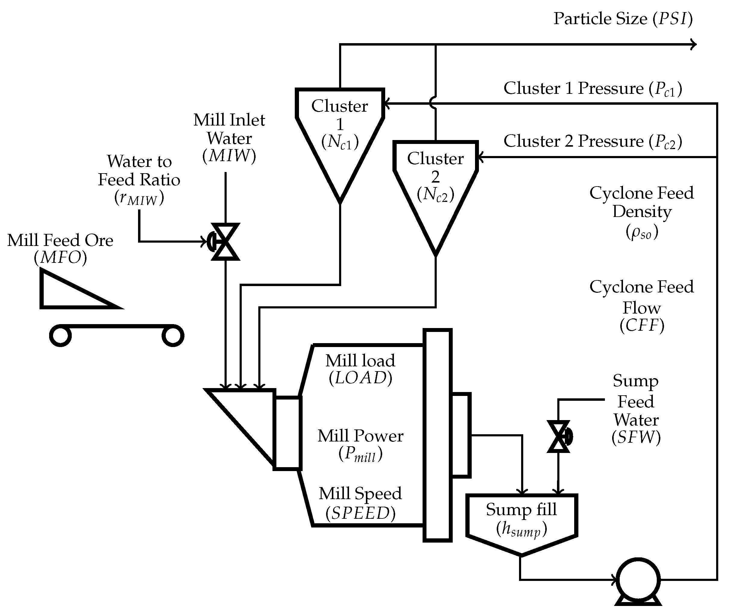
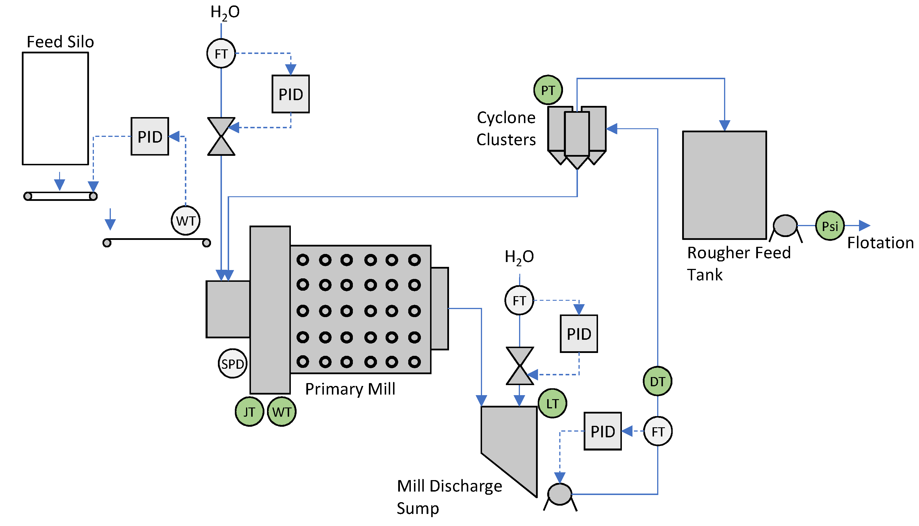
Figure 2 shows the manipulated variables (MVs) and controlled variables (CVs) as listed in Table 1. The primary milling circuit comprises of a 26 radius × 28 length ball mill with a wrap-around ABB motor and a variable speed drive (VSD). represents the power consumed by the mill, the variable rotational rate of the mill, and the total mill load as measured by load cells. As shown in Figure 3, fresh feed into the mill () is controlled by a proportional, integral, derivative (PID) controller that cascades to a VSD feeder under the silo. Water into the mill () is controlled as a ratio to the fresh feed (), cascading from a ratio controller to an inlet water PID controller. Both feed and water ratio set points are supplied by either the operator, from the Supervisory Control and Data Acquisition (SCADA) system, or the advanced process control (APC) system. The mill discharges through a partial overflow mechanism into the discharge sump. Two cyclone packs with 10 cyclones each in a duty/standby operating philosophy close the circuit loop. The coarse underflow is recycled back to the mill with the finer overflow reporting to the rougher feed surge tank and onto primary flotation. The APC also controls the discharge sump level (), discharge density (), and cyclone cluster pressure ( and ) by manipulating the discharge sump dilution water flow rate (), cyclone slurry flow rate (), and the number of open cyclones ( and ) in a cluster. The final product particle size passing 75 m () at the cyclone overflow is measured by a BlueCube analyzer. The advanced control strategy includes a layered approach consisting of PID, fuzzy logic-based and model predictive control, as described by Steyn et al. [14].
3.2. Process Data
The site uses a Siemens PCS7 programmable logic controller with a WinCC human–machine interface that connects to an OSI PI historian using Open Platform Communication. Analogue instrument data are logged to the database at a maximum frequency of 1 Hz. The primary mill data used during this project were sampled at a period of 2 min (0.008 Hz) over a duration of 23 weeks from the 1 September 2019 to the 10 February 2020.
The period was selected as it recorded an average process usage exceeding 90%. The period also incorporates data from before and after the mill online grind analyzer commissioning date of the 31 October 2019. From a control perspective, the data contain periods where the mill was under manual control as well as periods where the APC was active. Step tests to improve the dynamic step response models used by the model predictive control (MPC) algorithm of the APC were performed between the 1 and 3 February 2020. These data were collected at a one-minute frequency and is used in this study to derive models for comparison purposes.
3.3. Linear Empirical Models
The majority of industrial MPC systems use linear empirical models in their formulation [15]. Standard practice has been to develop these models by performing planned tests on the plant. These step-tests are designed to generate the data needed to produce linear models of the required fidelity. Performing a manual step test on a reasonable sized multi-variable controller represents a significant time investment, particular as engineer supervision is often required for the duration of the test. As an example, the controller employed on this plant has eight manipulated variables. Assuming a time to steady state of one hour and eight steps per variable are required, the total step test time may be calculated as,
If stepping can occur for eight hours per day, this is eight days of effort. The software vendors have introduced automated step testing software to assist in this area [16,17]. While these tools are definitely a boon to the MPC engineer, they still require that an initial model matrix (“seed matrix”) be derived for the system before the automated process can commence.
Linear Model Identification
Given a data set consisting of a set of inputs to a plant and the resulting outputs, several routines are available to derive the linear time-invariant models used in linear MPCs. Methods used include the following:
- Finite Impulse Response (FIR),
- Autoregressive with exogenous inputs (ARX) and
- subspace modeling (SS).
Further details of these algorithms are available in [15,18,19]. The FIR and ARX methods have the advantage of simplicity. Their disadvantage is that they are multi-input, single-output (MISO) methods and, therefore, do not take full advantage of the relationships in the data. In addition, these methods are not good at managing closed-loop data where the inputs are correlated [19]. Subspace models are less intuitive for the practitioner, but are multi-input, multi-output (MIMO) models by nature, and manage input correlation much better than the MISO methods.
For this study, FIR and SS methods are used. The particular SS method used is called canonical variate analysis (CVA) [20]. These methods are implemented in a commercially available package allowing for fast identification of multiple cases. For FIR, the user must specify a time to steady state (TTSS), the number of coefficients, and optionally a smoothing factor. A TTSS is supplied for the SS fits which is used for filtering purposes only. In addition, the maximum states per CV group and the maximum order per I/O pair can be specified. For this study, these parameters were left at their default values. If a CV is to be modeled as an integrating variable, this must be specified.
3.4. Semirigorous Mill Circuit Model
Apart from using a linear empirical model, the circuit in Figure 3 can also be model led using the semirigorous nonlinear population balance model of Le Roux et al. [21]. A brief overview of the model is given below. Table 1 shows the circuit variables, and Table 2 lists the model parameters.
For the purposes of this model, ore fragments too large to pass through the partial overflow mechanism are referred to as rocks and must be broken further. All ore fragments small enough to pass to the sump are referred to as solids. The broken ore below the specification size is referred to as fines. Note, whereas solids refer to all ore small enough to discharge from the mill, fines refer to the portion of solids smaller than the specification size. Therefore, solids are a combination of fine ore and coarse ore, where coarse ore refers to the portion of solids larger than the specification size.
3.4.1. Mill Model
The population volume balance model of the mill describes four states: water (), solids (), rocks (), and fines (),
where and represent the fraction of fines and rocks in , respectively; is the ore density; is the discharge rate; , , and are the cyclone underflow of water, solids, and fines, respectively; is a rock consumption term that indicates the volumetric rate of rocks broken into solids; and is a fines production term that indicates the volumetric rate of ore broken into fines. The mill inlet water is given by . The rheology factor is an empirically defined function that incorporates the effect of the fluidity and density of the slurry on the performance of the mill,
The fraction of the mill filled with charge () is given by,
where (m3) is the inside volume of the mill and is the volume of balls in the mill assumed as constant. Since the mill charge is measured by means of load cells, there is a linear relationship between and [22],
where and are calibration constants.
The mill power draw () is modeled as,
where is the power change parameter for the volume of mill filled, is the power change parameter for the volume fraction of solids in the slurry, is a normalization factor, and is the fraction of the mill filled at maximum power draw. The fraction of critical mill speed is calculated as [23]
where D is the internal mill diameter. The maximum mill power draw is parameterized as a linear function of [24],
where are function constants.
The rock consumption () and fines production () in (6)–(8) are defined as,
where is the rock consumption factor and indicates the energy required per tonne of rocks broken and is the fines production factor and indicates the energy required per tonne of fines produced. The fines production factor is modified by the fractional change in power per fines produced per change in fractional filling of the mill .
3.4.2. Sump Model
The population volume balance of the sump hold-ups, water (), solids (), and fines (), are defined as,
where the discharge flow-rates are,
The percentage of the sump filled with slurry () and the sump outflow density () are defined as,
where is the total sump volume and is the density of water.
3.4.3. Cyclone Cluster Model
The cluster of cyclones is modeled as a single classifier. If needed, the model can be expanded into separate smaller cyclones as in Botha et al. [25]. However, the goal here is simply to calculate the total water, solids, and fines split at the cluster.
The underflow of coarse material () is modeled as,
To determine the amount of water and fines accompanying the coarse underflow, the fraction of solids in the underflow () must be determined. This is modeled as,
where relates to the fraction solids in the underflow. The cyclone underflow flow rates in (5)–(8) are,
The product particle size is defined as the fraction of fines to solids in the cyclone overflow,
4. Data Quality Assessment Results
The DQA will be performed on two data sets available from the mill process. The first data set, which will be referred to as the “complete data set”, contains data for approximately one year. The second data set, which will be referred to as the “step data set”, contains a series of step tests on the same mill for a period in February 2020.
For the complete data set, there are sixteen variables of which was selected as the output. The other variables were candidates for being included as the inputs. For the step data set, there were 30 variables, of which the grinding rate, and the combined pressure of the two cyclones were selected as the key output variables. As can be seen from the mill circuit Figure 3, the two cyclones operate in parallel and not simultaneously. If one is on, then the other is off. Therefore, the combined pressure is simply the value of the on cyclone. The choice of variables is informed more by process knowledge than by any fundamental statistics; this is why different sets are chosen. It is an are for further research on how to choose the best inputs and outputs for the algorithm.
4.1. Analysis of the Complete Data Set
The analysis of the complete data set can be split into two parts: correlation analysis and data segmentation. Correlation refers to the absolute value of the standard Pearson’s correlation. A signal is assumed to be correlated if Pearson’s correlation is greater than 0.90.
4.1.1. Correlation Analysis of the Complete Data Set
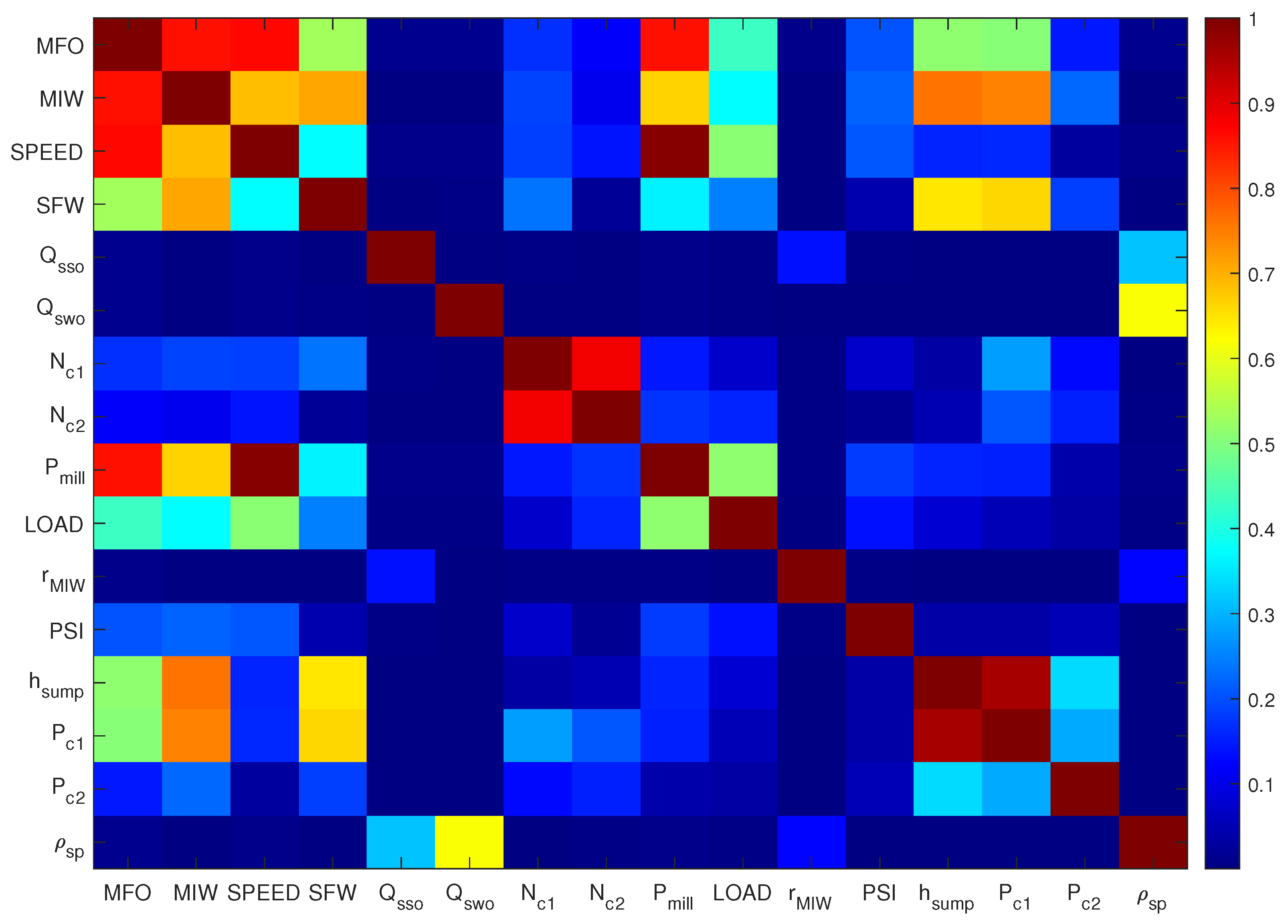
Figure 4 shows the cross-correlation plot for all the variables. The x-axis has the same labeling as the y-axis. The color scale ranges from deepest blue which corresponds to a correlation of zero to deepest red which corresponds to a perfect correlation of 1. Variables that are in shades of dark red are correlated with one another. From Figure 4, it can be seen that the first three variables as well as the ninth variable are strongly correlated with each other. Likewise, the eighth and ninth variables are strongly correlated with each other. Finally, the fourteenth and fifteenth variables are also strongly correlated with one another. This means that only one out of each group of variables should be used when it comes to the data segmentation task.
4.1.2. Data Segmentation for the Complete Data Set
In order to investigate the effects of correlation on the data segmentation results, the following cases will be considered:
- Case 1: Here the partitioning will be performed using , , , and (that is, the first four variables).
- Case 2: Here the partitioning will be performed using only .
- Case 3: Here the partitioning will be performed using only , , and .
- Case 4: Here the partitioning will be performed using only , which is a quasi-integrating variable.
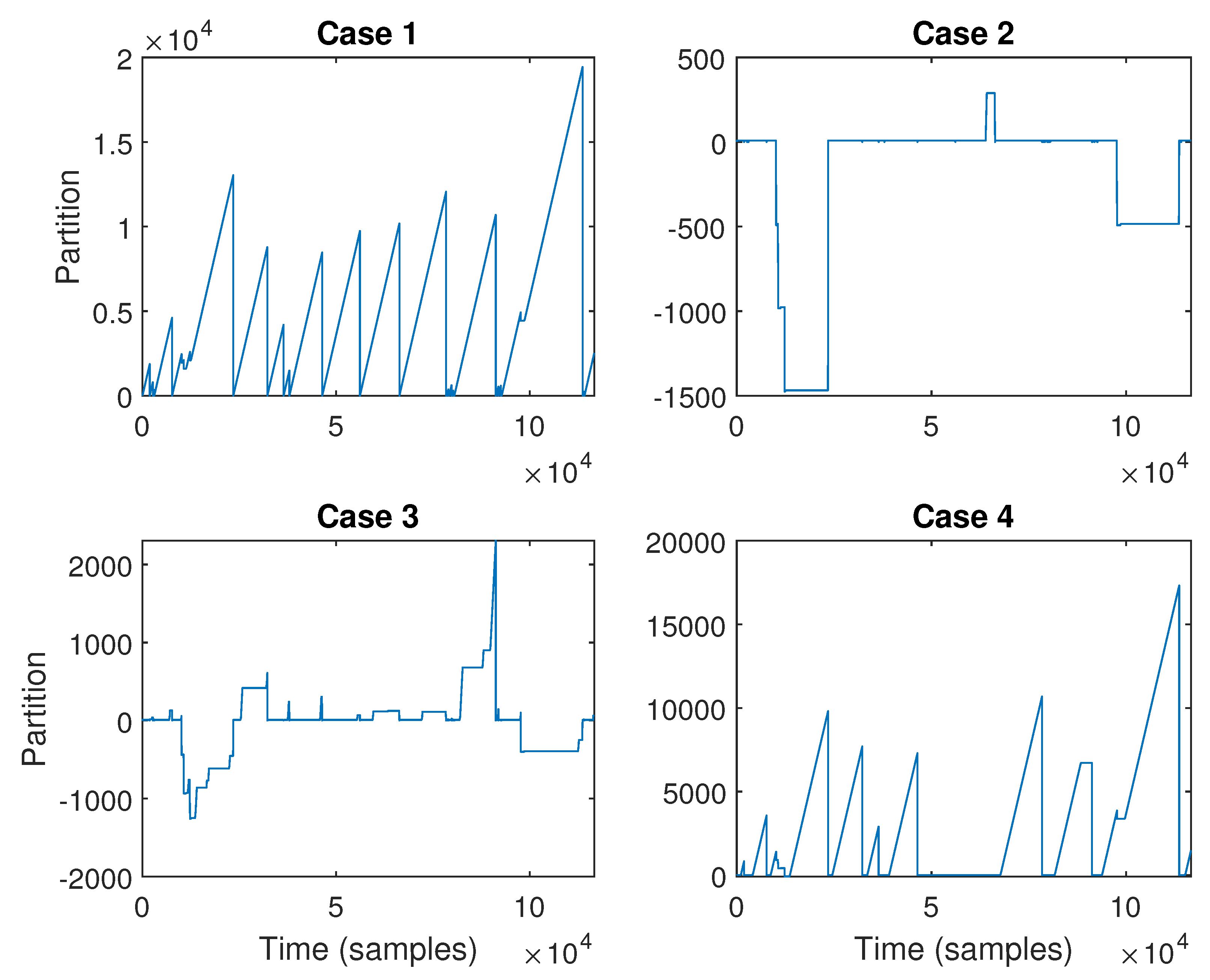
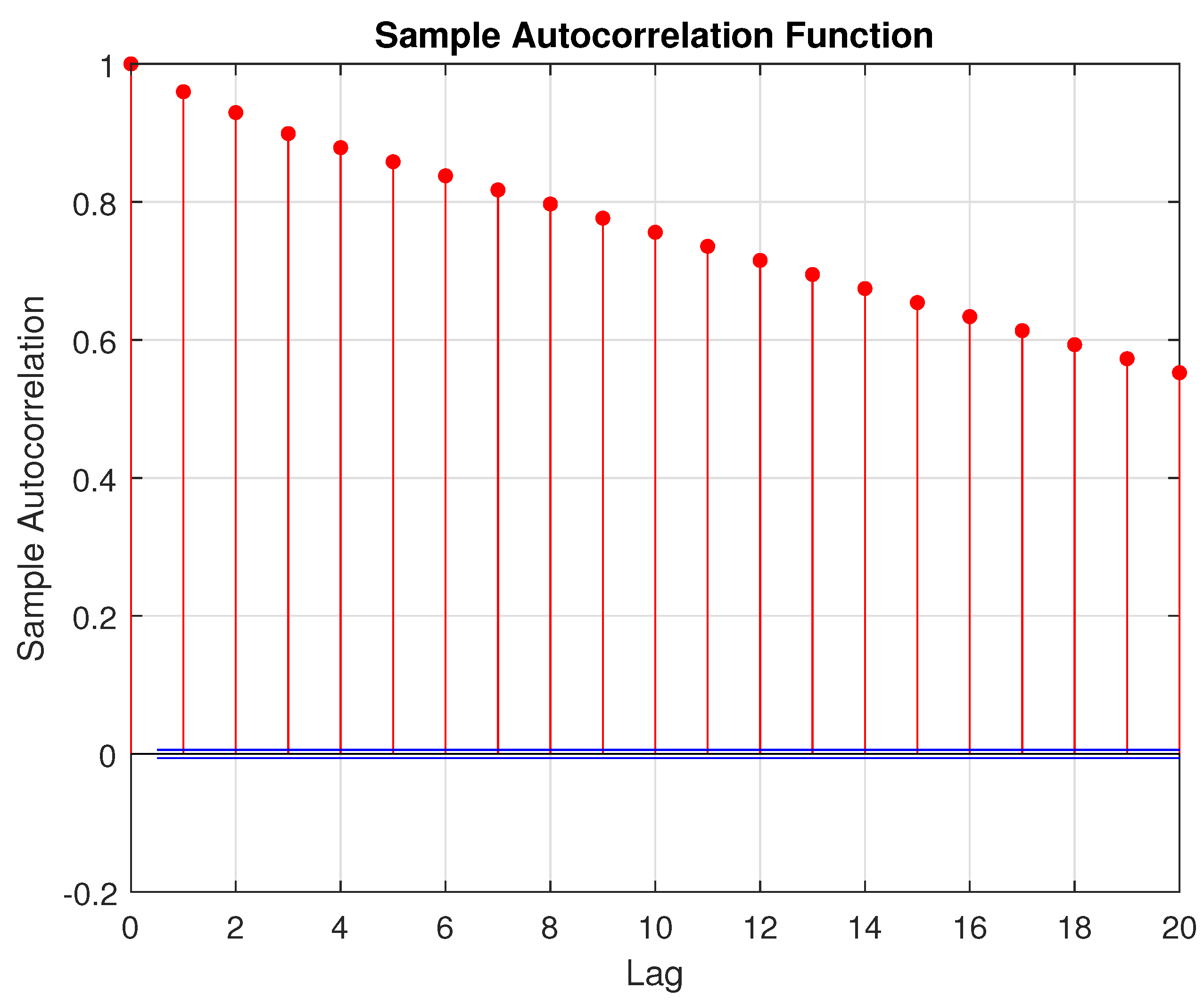
Figure 5 shows the partition results for all four cases. The x-axis is the time in units of samples from the initial time period, while the y-axis shows the partition number. Adjacent times with the same partition number can be assumed to belong to the “same” model. A line implies that the data are not sufficiently excited or good for modeling. Regions with the same or similar partition number separated by a small region can also be assumed to belong to the same overall model. From Figure 5 (top left), which shows the results for Case 1, it can be seen that using the first four variables provides no regions that are suitable for system identification. This is a direct consequence of the fact that the selected variables are correlated with each other forcing the information matrix to be uninvertible. This clearly shows the issues involved with multivariate data segmentation. Figure 5 (top right) presents the partition results for Case 2. It can be seen that using only a single variable provides results that suggest there is a relatively large chunk of data that could potentially be considered to not only come from a single model, but also be sufficiently excited for modeling. These data will then be used in the next section for modeling to examine the effect of the segmented data on the overall models obtained for both linear and nonlinear situations. Figure 5 (bottom left) shows the partition results for Case 3. It can be noted that although there is some correlation in the data set, it is perhaps possible to obtain something useful. This will test what the effect of correlation is on the data segmentation. From Figure 5 (bottom left), it can be seen that using three variables for partitioning gives similar results to using a single variable. With the increase in variables, there are now more individual partitions. Nevertheless, it can be seen that this case is very similar to that with only one partitioning variable (cf. Figure 5 (top right)). Further, note that it would seem that the third variable is the troublesome variable that is correlated with the other variables. Furthermore, it should be noted that strictly speaking any linear combination of variables is problematic. However, such a circumstance will not be found using a simple correlation plot. As well, there is a need to consider time-delayed variables and their lagged cross-correlation. Finally, Figure 5 (bottom right) shows the partition results for Case 4. It can be noted that with an integrating input, it is necessary to preprocess the signal by integrating it. The integrating nature of the signal is quite clear from the autocorrelation plot shown in Figure 6. Here, it can be noted that the autocorrelation plot shows a typical pattern associated with an integrating or autoregressive process, where the values decrease steadily, but there is no cut-off point [6]. For an integrating process, it would be expected that the values remain more or less constant at 1 [6]. In practice, due to sampling issues, it may not be possible to see such a behaviour. Instead, the values will decrease as seen here. From Figure 5 (bottom right), it can be seen that the partitioning results are similar to that obtained before showing that the selection of variables, although critical, is not necessarily all that important. As long as appropriately uncorrelated variables are selected, relatively similar results are obtained.
4.2. Data Quality Assessment for the Step Data Set
Using the step data set for DQA shows similar results to the previous case. Noted that as a step test can often provide sufficient excitation for modeling a process, much of the data set is selected as being valid. However, the results strongly depend on the variables selected, since as before, some of the variables are strongly correlated with each other. As the overall results are the same as before, they are not provided here.
5. Results
The models discussed above were used with the two sets of data to generate two linear and two nonlinear models.
5.1. Results from the Routine Operating Data
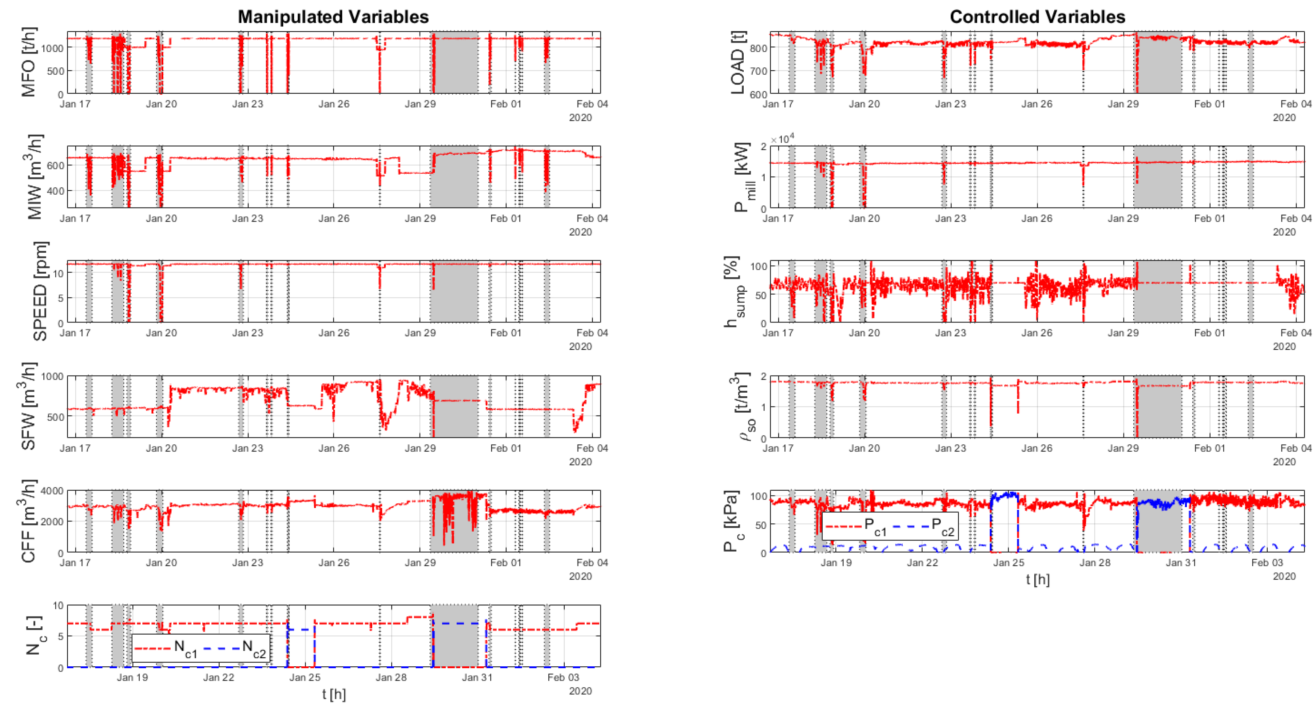
DQA indicates that a section of data consisting of a little over 19 days of data was suitable for identification. The modeled system MVs and CVs for this period are shown in Figure 7.
The light gray vertical shading in the figures indicates that data has been excluded from the fitting for all variables. The dark gray shading indicates that data for that variable only has been excluded.
5.1.1. Results Using the Linear Empirical Models
The fitting routine defines cases consisting of a set of MVs and CVs. If any variable in the set is excluded or has bad data the fit is not performed for all variables. For CVs, this effect can be minimized by identifying them one by one. This is not recommended for the SS algorithm, which takes advantage of the correlation structure of the CVs. The DQA model includes the number of cyclones open in the pack as an MV.
It would be tempting to include the flow out of the sump as an independent variable for modeling. Analysis shows that this total flow out of the sump is not an independent variable, as it is used in closed-loop control of the sump level.
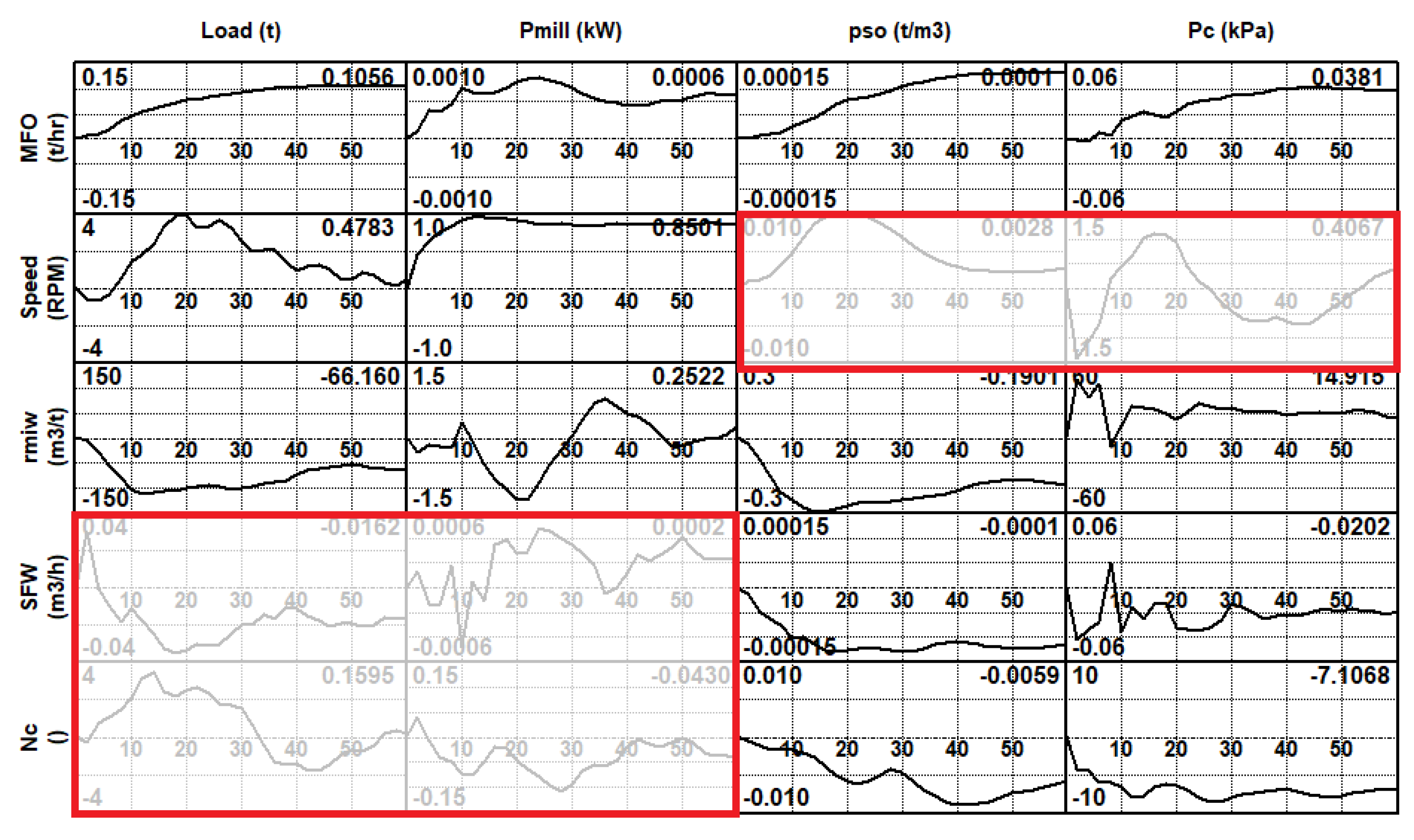
The calculated models for the data shown in Figure 7 are shown in Figure 8. The CVA method was used to generate a matrix of SS models for the system. The linear time-invariant models are represented as unit step responses, i.e., the response of the output variable (columns of the matrix) to a step of one engineering unit of the input (rows of the matrix) at time zero. The timescales are in minutes, and the response curves are in engineering units. The number in the top right corner of each plot is the gain of that particular model, or the steady-state value.
More analysis of these models will be presented below, where they are compared with models derived from planned step test data. Suffice it to say that some key linear models such as feed and speed to load, speed to power, feed, inlet and sump water to density and feed, and number of cyclones to cyclone pressure have been identified successfully.
A further point to note is that not all models calculated are implemented in the seed models used to bootstrap an automated stepping campaign. The reason for this is that if the models are not well known, then weak directions need to be avoided. The models that would be deleted are shown with red boxes around them in Figure 8. The load and power to sump feed water and number of cyclones to inlet water ratio models would be removed on physical grounds. The discharge density and cyclone pressure to speed model would be removed on the basis of small scaled gains. The resulting matrix would be robust enough for seed model purposes.
5.1.2. Results Using the Semirigorous Mill Circuit Model
The model parameters for the model presented in Section 3.4 can be estimated from the routine operating process data representing a steady-state operating condition. In other words, it is necessary to estimate parameters for data where the MVs and CVs remain constant such that in (5)–(8) and (17)–(19). The estimation procedure follows an algebraic routine to sequentially determine the parameters in Table 2. Although it is advantageous that the model be fitted to a single steady-state operating condition, the procedure is dependent on accurate process measurements. Any unmeasured spillage water added at the sump has a significant impact on the simulation accuracy of the model. If this additional water is not accounted for, the model may predict that the sump will run dry very quickly. The model accuracy is also dependent on a good characterization of . Specifically, it is important to have a reasonably accurate parameterization of in (14) and to know if the plant is operating either before or past the peak in [22,24]. Once the model states and parameters are determined for the specific steady-state operating condition, pure simulation is used to produce the model outputs.
5.2. Results from the Planned Step Tests
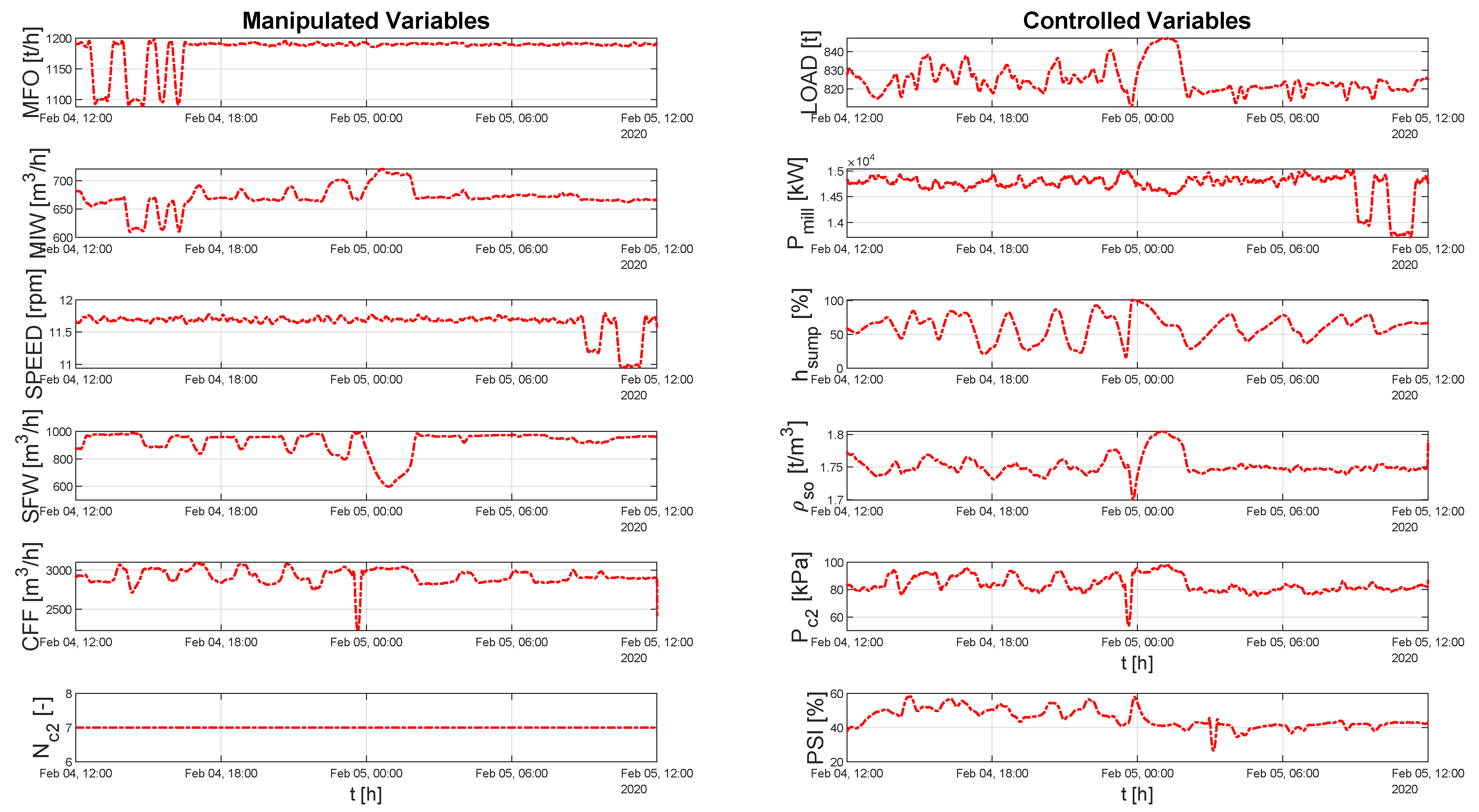
As discussed above, planned step tests were made on the process. The key system MVs and CVs for this period are shown in Figure 9.
5.2.1. Results Using the Linear Empirical Model
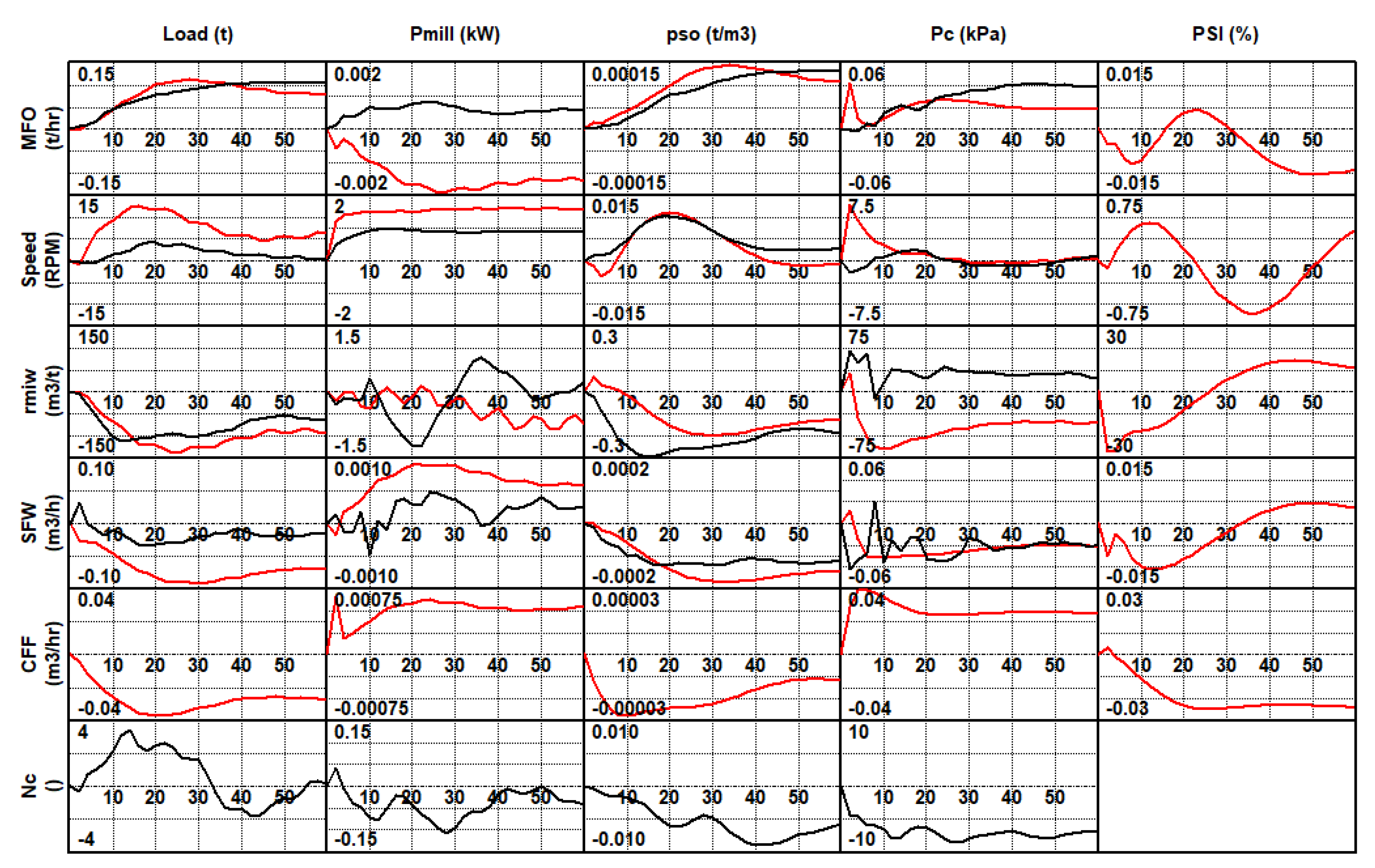
The planned step data is particularly suitable for identifying linear dynamic models, as the inputs tend to be uncorrelated. The CVA method was used to generate a matrix of SS models for the system. The results are shown in Figure 10, where they are overlaid with the models calculated from the planned steps. Note that no steps were made on the number of cyclones in operation, so this variable is excluded from the models. It would be usual to delete some of these curves based on either physical intuition or small gains. This has not been done here to retain all the curves for comparison with those calculated from the DQA-determined data.
Visually, it is clear that there is reasonable agreement between these models in some cases, but there are some that agree poorly. To quantify this, the ratio of the gains of the DQA model to the planned step tests model is formed for each submodel. The results are shown in Table 3.
Assuming the planned step test model is accurate, a negative gain ratio means that the DQA model could potentially cause instability if used for process control. From experience, gains that are up to twice as large or as small can be tolerated, particularly if used as seed models. In this case, of the twelve models six have acceptable gain ratios, three have negative gain ratios, one has a ratio less than 0.5 and one a little higher than two.
5.2.2. Results Using the Semirigorous Mill Circuit Model
Similarly to Section 5.1.2, the parameter fitting procedure used to fit the semirigorous model to the data identified by DQA was used for the planned step test data. The only change necessary was to reparameterise in (14).
5.3. Comparison of the Linear and Nonlinear Models
Although not the primary objective of this work, the availability of a linear, data-driven, and semirigorous, fundamentally driven dynamic model of the plant invites comparison between the accuracy and utility of the two approaches.
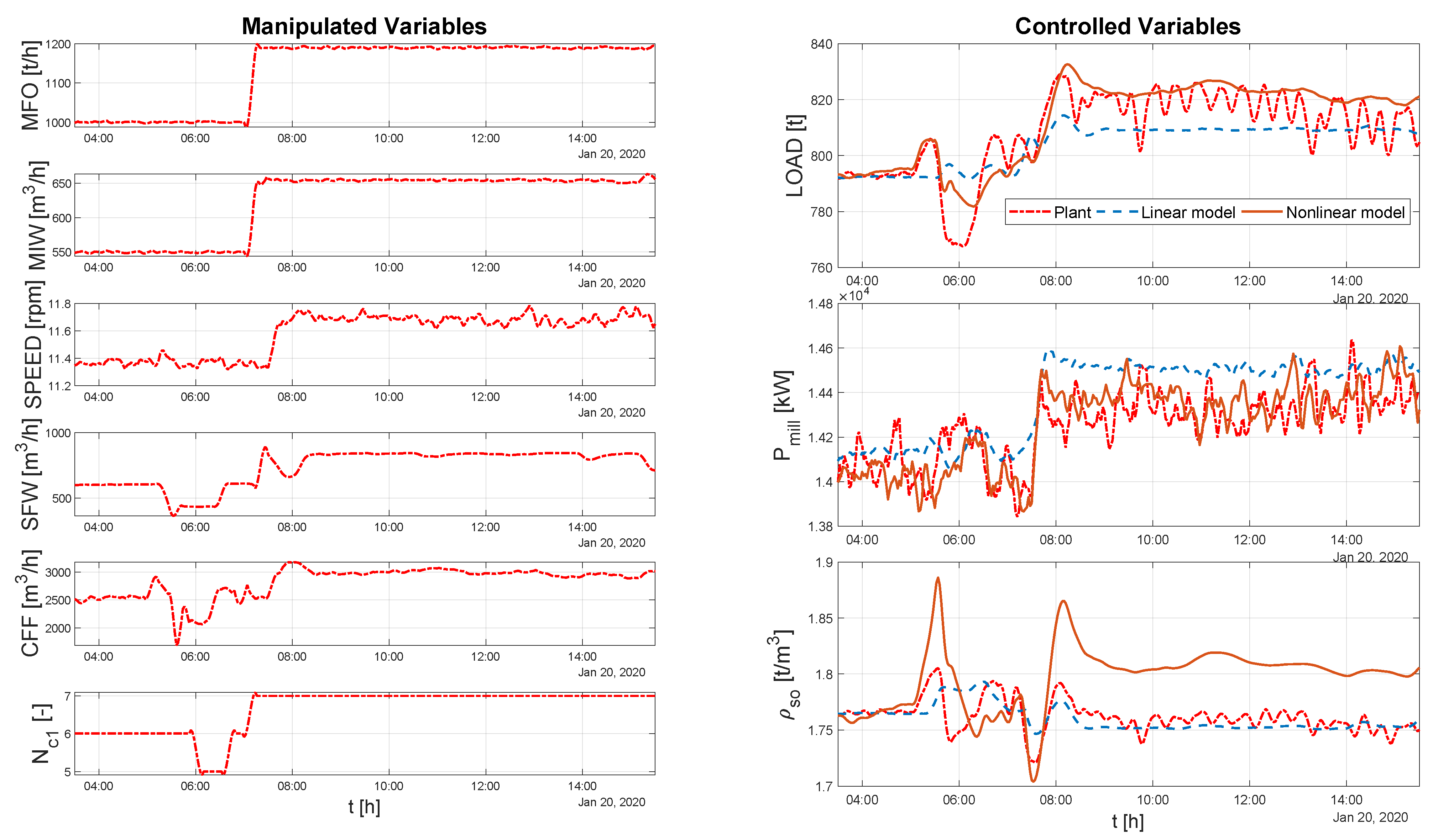
The results from modeling the DQA data is used to compare the two models. The visual comparison of the predictions of the two models is shown in Figure 11.
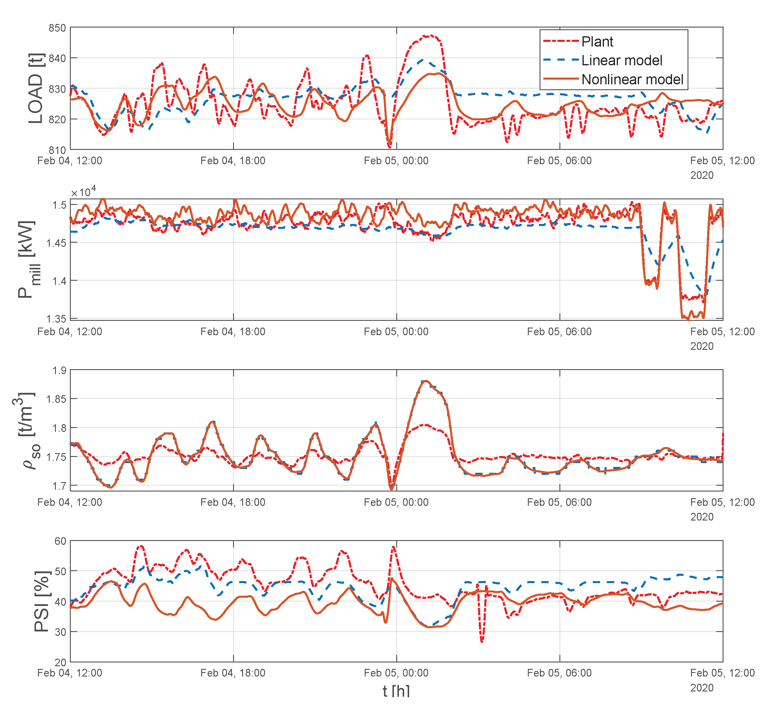
The results from modeling the planned step test data are used to compare the two models. The visual comparison of the predictions of the two models is shown in Figure 12.
The goodness-of-fit statistics for the two models are given in Table 4. All the models have small mean squared errors (MSEs). The correlation coefficient for the power () and discharge density () are very good, but poorer for the load () and, in particular, the grind (). The nonlinear model gives a superior prediction of the discharge density and load. Further investigation would be needed to determine why the grind predictions are poor, as this could be due to either an unmodelled effect or a fault in the instrument.
6. Conclusions
With the increasing need for automated data processing methods, this paper examined the application of a DQA method in comparison with planned step tests, linear, and nonlinear models of the system. First, it was shown that for multivariate DQA one of the challenges is selecting the appropriate set of variables for partitioning. Nevertheless, the DQA method was able to uncover a large region of data suitable for modeling. Second, it was shown that both the linear and nonlinear models of the primary mill can use the identified region for modeling. In addition, planned step test data was also used and compared. However, it was shown that the closed-loop data obtained using the DQA method provided poorer estimates than the planned step tests. This can partly be explained by noting that such closed-loop data presents a number of challenges for identification. Nevertheless, the models obtained would have been sufficient as the initial seed models for the automated APC methods. Future work will consider extending the applicability of the DQA method to more complex situations with the eventual goal of being able to better identify appropriate regions from complex industrial data sets and apply it to various different types of models.
Author Contributions
Conceptualization, K.B. and Y.A.W.S.; Data curation, C.S.; Formal analysis, K.B., D.l.R., Y.A.W.S. and C.S.; Investigation, K.B., D.l.R., Y.A.W.S. and C.S.; Methodology, K.B., D.l.R. and Y.A.W.S.; Validation, K.B., D.l.R., Y.A.W.S. and C.S.; Visualization, K.B., D.l.R., Y.A.W.S. and C.S.; Writing—review and editing, K.B., D.l.R., Y.A.W.S. and C.S.; All authors have read and agreed to the published version of the manuscript.
Funding
This research received no external funding.
Institutional Review Board Statement
Not applicable.
Informed Consent Statement
Not applicable.
Data Availability Statement
The industrial data presented in this study is not publicly available.
Conflicts of Interest
The authors declare no conflict of interest.
Abbreviations
The following abbreviations are used in this manuscript:
| APC | Advanced Process Control |
| ARX | Autoregressive with exogenous inputs |
| CVA | Canonical Variable Analysis |
| CV | Controlled Variable |
| DQA | Data Quality Assessment |
| FIR | Finite Impulse Response |
| I/O | Input/Output |
| MIMO | Multi-input, Multi-output |
| MISO | Multi-input, Single-Output |
| MPC | Model Predictive Control |
| MSE | Mean Squared Error |
| MV | Manipulated Variable |
| PID | Proportional, Integral, Derivative |
| SS | Subspace |
| TTSS | Time to steady state |
| SCADA | Supervisory Control and Data Acquisition |
| VSD | Variable Speed Drive |
References
- Ge, Z.; Song, Z.; Ding, S.X.; Huang, B. Data Mining and Analytics in the Process Industry: The Role of Machine Learning. IEEE Access 2017, 5, 20590–20616. [Google Scholar] [CrossRef]
- McCoy, J.; Auret, L. Machine learning applications in minerals processing: A review. Miner. Eng. 2019, 132, 95–109. [Google Scholar] [CrossRef]
- Lidwell, W.; Holden, K.; Butler, J. Universal Principles of Design, Revised and Updated: 125 Ways to Enhance Usability, Influence Perception, Increase Appeal, Make Better Design Decisions, and Teach through Design; Rockport Pub: Beverly, MA, USA, 2010. [Google Scholar]
- Qin, S.J. Process data analytics in the era of big data. AIChE J. 2014, 60, 3092–3100. [Google Scholar] [CrossRef]
- Ljung, L. System Identification: Theory for the User; Prentice Hall Inc.: Upper Saddle River, NJ, USA, 1999. [Google Scholar]
- Shardt, Y.A.W. Statistics for Chemical and Process Engineers; Springer: Berlin, Germany, 2015. [Google Scholar]
- Peretzki, D.; Isaksson, A.; Carvalho Bittencourt, A.; Forsman, K. Data Mining of Historic Data for Process Identification; Linköping University Electronic Press: Linköping, Sweden, 2011. [Google Scholar]
- Shardt, Y.A.W.; Huang, B. Data quality assessment of routine operating data for process identification. Comput. Chem. Eng. 2013, 55, 19–27. [Google Scholar] [CrossRef]
- Arengas, D.; Kroll, A. A data selection method for large databases based on recursive instrumental variables for system identification of MISO models. In Proceedings of the 2019 18th European Control Conference (ECC), Naples, Italy, 25–28 June 2019; pp. 357–362. [Google Scholar]
- Shardt, Y.A.; Yang, X.; Brooks, K.; Torgashov, A. Data Quality Assessment for System Identification in the Age of Big Data and Industry 4.0. IFAC-PapersOnLine 2020, 53, 104–113. [Google Scholar] [CrossRef]
- Shardt, Y.A.W. Data Quality Assessment for Closed-Loop System Identification and Forecasting with Application to Soft Sensors. Ph.D. Thesis, University of Alberta, Edmonton, AB, Canada, 2012. [Google Scholar]
- Shardt, Y.A.W.; Brooks, K.S. Automated system identification in mineral processing industries: A case study using the zinc flotation cell. IFAC-PapersOnLine 2018, 51, 132–137. [Google Scholar] [CrossRef]
- Shah, S.; Shardt, Y.A.W. Segmentation methods for model identification from historical process data. IFAC-PapersOnLine 2014, 47, 2836–2841. [Google Scholar]
- Steyn, C.W.; Brooks, K.S.; De Villiers, P.G.R.; Muller, D.; Humphries, G. A holistic approach to control and optimization of an industrial run-of-mine ball milling circuit. IFAC Proc. Vol. 2010, 43, 137–141. [Google Scholar] [CrossRef]
- Qin, S.J.; Badgwell, T.A. A survey of industrial model predictive control technology. Control Eng. Pract. 2003, 11, 733–764. [Google Scholar] [CrossRef]
- Kalafatis, A.; Patel, K.; Harmse, M.; Zheng, Q.; Craik, M. Multivariable step testing for MPC projects reduces crude unit testing time. Hydrocarb. Process. 2006, 85, 93–100. [Google Scholar]
- Nieto, L.; Olivares, J.; Gatica, J.; Ramos, B.; Olmos, H. Implementation of a multivariable controller for grinding-classification process. IFAC Proc. Vol. 2009, 42, 55–60. [Google Scholar] [CrossRef]
- Jamaludin, I.; Wahab, N.; Khalid, N.; Sahlan, S.; Ibrahim, Z.; Rahmat, M.F. N4SID and MOESP subspace identification methods. In Proceedings of the 2013 IEEE 9th International Colloquium on Signal Processing and its Applications, Kuala Lumpur, Malaysia, 8–10 March 2013; pp. 140–145. [Google Scholar]
- Zhao, H.; Harmse, M.; Guiver, J.; Canney, W.M. Subspace identification in industrial APC applications—A review of recent progress and industrial experience. IFAC Proc. Vol. 2006, 39, 1074–1079. [Google Scholar] [CrossRef]
- Larimore, W.E. Automated multivariable system identification and industrial applications. In Proceedings of the 1999 American Control Conference (Cat. No. 99CH36251), San Diego, CA, USA, 2–4 June 1999; Volume 2, pp. 1148–1162. [Google Scholar]
- Le Roux, J.D.; Craig, I.K.; Hulbert, D.G.; Hinde, A.L. Analysis and validation of a run-of-mine ore grinding mill circuit model for process control. Miner. Eng. 2013, 43–44, 121–134. [Google Scholar] [CrossRef] [Green Version]
- Powell, M.S.; Van der Westhuizen, A.P.; Mainza, A.N. Applying grindcurves to mill operation and optimisation. Miner. Eng. 2009, 22, 625–632. [Google Scholar] [CrossRef]
- Apelt, T.A.; Asprey, S.P.; Thornhill, N.F. Inferential measurement of SAG mill parameters. Miner. Eng. 2001, 14, 575–591. [Google Scholar] [CrossRef]
- Le Roux, J.D.; Steinboeck, A.; Kugi, A.; Craig, I.K. Steady-state and dynamic simulation of a grinding mill using grind curves. Miner. Eng. 2020, 152, 106208. [Google Scholar] [CrossRef]
- Botha, S.; Craig, I.K.; Le Roux, J.D. Hybrid non-linear model predictive control of a run-of-mine ore grinding mill circuit. Miner. Eng. 2018, 123, 49–62. [Google Scholar] [CrossRef] [Green Version]
Figure 1.
A high-level process flow diagram of the platinum concentrator plant.

Figure 2.
Primary milling circuit with manipulated and controlled variables.

Figure 3.
Simplified process flow diagram of the primary milling circuit.

Figure 4.
Cross-correlation plot for the complete data set.

Figure 5.
Data Segmentation for (top left) Case 1, (top right) Case 2, (bottom left) Case 3, and (bottom right) Case 4.
Figure 5.
Data Segmentation for (top left) Case 1, (top right) Case 2, (bottom left) Case 3, and (bottom right) Case 4.

Figure 6.
Sample autocorrelation for the level .

Figure 7.
MVs and CVs for the DQA data.

Figure 8.
Linear model matrix for DQA data.

Figure 9.
MVs and CVs for the planned step test data.

Figure 10.
Linear time- invariant models from planned step tests (red) and DQA data (black).

Figure 11.
Comparison of the CV predictions using the linear and nonlinear models for a short section of DQA data.
Figure 11.
Comparison of the CV predictions using the linear and nonlinear models for a short section of DQA data.

Figure 12.
Comparison of the CV predictions using the linear and nonlinear models for the planned step test data.
Figure 12.
Comparison of the CV predictions using the linear and nonlinear models for the planned step test data.


Table 1.
Manipulated and controlled variables in the primary milling circuit.
| Variable | Unit | Description |
|---|---|---|
| Manipulated Variables | ||
| t/h | Fresh mill feed ore tonnage | |
| m3/h | Mill inlet water | |
| m3/t | Mill inlet water to feed ore ratio | |
| rpm | Mill speed | |
| m3/h | Sump feed water | |
| m3/h | Cyclone feed flow-rate | |
| integer | Number of cyclones in operation for cluster 1 | |
| integer | Number of cyclones in operation for cluster 2 | |
| Controlled Variables | ||
| ton | Mill load | |
| MW | Mill power | |
| % | Percentage of sump filled with slurry | |
| t/m3 | Sump outflow density | |
| kPa | Cyclone cluster 1 pressure | |
| kPa | Cyclone cluster 2 pressure | |
| % pass 75 mm | Product particle size passing 75 m | |
Table 2.
Model parameters.
| Parameter | Unit | Description |
|---|---|---|
| General | ||
| t/m3 | Density of ore | |
| t/m3 | Density of water | |
| Mill | ||
| - | Mass fraction of fines in the feed ore | |
| - | Mass fraction of rocks in the feed ore | |
| D | m | Internal mill diameter |
| - | Power parameter for fraction solids in the mill | |
| - | Power parameter for volume of mill filled | |
| h | Discharge rate | |
| - | Rheology normalization factor | |
| - | Fraction of mill volume filled at maximum power draw | |
| MWh/t | Fines production factor | |
| - | Fractional change in fines production factor per change in fractional mill filling | |
| MWh/t | Rock consumption factor | |
| MW | Maximum mill power draw parameters | |
| m3 | Mill volume | |
| Sump | ||
| m3 | Sump volume | |
| Cyclone cluster | ||
| - | Parameter related to fraction solids in cyclone underflow | |
| - | Cyclone model constant | |
| m3/h | Parameter related to coarse split at cyclone | |
Table 3.
Ratio of gains between the DQA and planned step test models. Red background—negative; Orange background—greater than two; Yellow background—positive, less than 0.5.
Table 3.
Ratio of gains between the DQA and planned step test models. Red background—negative; Orange background—greater than two; Yellow background—positive, less than 0.5.
| 1.35 | −0.36 | 1.24 | 2.03 | |
| 0.08 | 0.54 | N/A | N/A | |
| 0.70 | −0.34 | 1.45 | −0.42 | |
| N/A | N/A | 0.80 | 0.93 |
Table 4.
Goodness-of-Fit Statistics.
| Average | 824.9 | 14.73 | 1.752 | 0.447 |
| MSE—Nonlinear model | 6.17 | 0.14 | 0.002 | 0.082 |
| —Nonlinear model | 0.32 | 0.86 | 0.98 | 0.05 |
| MSE—Linear Model | 7.06 | 0.10 | 0.028 | 0.055 |
| —Linear Model | 0.22 | 0.87 | 0.79 | 0.12 |
Publisher’s Note: MDPI stays neutral with regard to jurisdictional claims in published maps and institutional affiliations. |
© 2021 by the authors. Licensee MDPI, Basel, Switzerland. This article is an open access article distributed under the terms and conditions of the Creative Commons Attribution (CC BY) license (https://creativecommons.org/licenses/by/4.0/).
Share and Cite
MDPI and ACS Style
Brooks, K.; le Roux, D.; Shardt, Y.A.W.; Steyn, C. Comparison of Semirigorous and Empirical Models Derived Using Data Quality Assessment Methods. Minerals 2021, 11, 954. https://0-doi-org.brum.beds.ac.uk/10.3390/min11090954
AMA Style
Brooks K, le Roux D, Shardt YAW, Steyn C. Comparison of Semirigorous and Empirical Models Derived Using Data Quality Assessment Methods. Minerals. 2021; 11(9):954. https://0-doi-org.brum.beds.ac.uk/10.3390/min11090954
Chicago/Turabian StyleBrooks, Kevin, Derik le Roux, Yuri A. W. Shardt, and Chris Steyn. 2021. "Comparison of Semirigorous and Empirical Models Derived Using Data Quality Assessment Methods" Minerals 11, no. 9: 954. https://0-doi-org.brum.beds.ac.uk/10.3390/min11090954
Note that from the first issue of 2016, this journal uses article numbers instead of page numbers. See further details here.