Inversion and Uncertainty Estimation of Self-Potential Anomalies over a Two-Dimensional Dipping Layer/Bed: Application to Mineral Exploration, and Archaeological Targets

Abstract

Self-Potential data have been widely used in numerous applications. The interpretation of SP data from subsurface bodies is quite challenging. The advantages of geophysical inversion for interpreting non-linear geophysical problems have gained a great deal of attention over conventional interpretation. The efficiency of the present inversion approach in interpreting SP anomalies from a thin dipping layer/bed is presented in the study. The inversion approach was applied to interpret synthetic model parameters such as the self-potential of the layer (k), depth to the body top (h), location of the body (x₀), dip angle ($\theta ),$ and the upper and lower end of the sheet (δ₁ and δ₂). The interpretation of the results showed that the parameters Δh, δ₁, and δ₂ exhibited a wide range of results. The estimated parameter values lay within the limit of uncertainty. The inversion approach was also applied to two field datasets obtained from polymetallic deposits in Russia and Azerbaijan for mineral exploration purposes and one from a buried ancient Roman limestone construction in Halutza, Israel, for the purposes of archaeological study. The field investigation results demonstrate a good agreement with previous works of literature. The efficiency of the present approach for interpreting SP anomalies from thin layer/bed-like structures is shown in this study.

1. Introduction

The Self-Potential (SP) method is one of the oldest geoelectrical methods for measuring the natural electric potentials formed on the surface of the earth as a result of different mechanisms. The SP method was initially used for metalliferous sulfide deposits [1], and then in different branches of exploration and applied geophysics, such as the fields of mining [2,3] and archaeological investigation [4,5,6]. SP methods have also been applied in numerous other applications, such as hydrology, engineering, environmental monitoring, volcanology, and the identification of shear zones [7,8,9,10,11,12,13].

Many qualitative and quantitative methods have been developed for the interpretation of SP anomalies, from simple geometrical shapes to 2D and 3D geological structures [12,14]. SP data interpretation is based on field SP anomalies or the computed models from idealized structures or 2D or 3D geological structures with irregular shapes and sizes [13]. Many interpretation techniques have been established to interpret SP data by identifying simple geometric source bodies. Such bodies may be embedded in a homogeneous and isotropic half-space or in layered or faulted geometries [15]. Subsurface structures characterized by spheres or vertical and horizontal cylinders have been interpreted using various techniques [16,17,18,19,20,21,22,23,24,25,26,27,28,29,30]. Interpretation of SP anomalies from 2D thin and thick sheets has also been performed using different interpretation techniques [13,19,31,32,33,34,35,36,37,38,39,40,41,42,43,44,45,46,47,48]. In fact, 2D inclined plate-type structures from SP anomalies have also been interpreted using a number of techniques [14,49,50,51]. Detailed techniques for the interpretation of SP anomalies have been reported [7,13,51]. However, the interpretation of SP anomalies from a 2D thin dipping layer/bed has not been well studied in most of the literature, as mentioned above.

Self-Potential interpretation can be performed either based on an analysis of the signal or using various inversion approaches. Various interpretation techniques, such as characteristic points, logarithmic curve matching, and nomograms, have been developed previously [16,17,19,31,52,53]. These qualitative interpretation methods were mostly trial-and-error methods, which have a higher error with respect to interpretation. The interpretation of SP anomalies has subsequently been performed using practical techniques and inversion methods [14,24,32,36,38,54,55]. However, while these techniques also give efficient results, only a few parameters can be estimated, leading to incorrect interpretations of all of the model parameters. Since SP anomalies are generally non-linear, many new techniques have been established based on the non-linear inversion of SP anomalies. It is well known that the inversions of SP anomalies are also ill-posed, and non-uniqueness is inherent in the interpretation; therefore, superior approaches and competent algorithms are required to invert all the model parameters [13]. In recent decades, non-derivative nature-inspired global optimization and metaheuristics have become prevalent, rather than using derivative-based local-search optimization to resolve geophysical inverse problems [56,57]. SP data have been interpreted using various global optimization algorithms, including genetic algorithms [23], neural network [28], particle swarm optimization [39,58], differential evolution [59,60], ant colony optimization [61], black-hole algorithm [62], genetic-price algorithm [27], and micro differential evolution algorithm [63]. These optimization algorithms have been well applied in the interpretation of idealized bodies such as spheres, horizontal and vertical cylinders, and thin and thick sheets for SP data. However, in none of the above literature has the interpretation of 2D dipping layers been studied using a non-linear inversion approach to interpret all model parameters.

Hence, in this work, we employ the forward modeling approach of [41] for the interpretation of SP anomalies produced from a 2D thin dipping layer. The 2D thin dipping layers and bed-type structures are very important in locating the different geological layers associated with mineralization or any specific structures associated with it. Moreover, the work in [41] is based on a combination of automatic linear and non-linear approaches to interpreting all of the model parameters, but the uncertainty in the interpretation of such models has not been studied at all. In every geophysical optimization, the estimation of the uncertainty of the model parameters is very important for achieving precise interpretation results. This also determines the relationship among the model parameters and how each parameter influences the others in the final interpretation. Hence, the current work focuses on the interpretation of all model parameters associated with thin dipping layers and the uncertainty associated with the interpretation of all model parameters, which has not been studied for such types of structures. Here, we used the non-linear global optimization of a very fast simulated annealing (VFSA) technique for the elucidation of SP anomalies. The VFSA approach does not involve a priori evidence for the understanding of SP data. The advantage of this method is that it is able to effectively interpret both small and large profile data, for solitary as well as multiple structures, and it is able to accurately interpret the parameters of near-surface as well as deeper structures. This approach is illustrated and evaluated on synthetic and noisy models, as well as on three field anomalies for polymetallic deposits from Russia and Azerbaijan, in addition to archaeological investigations from Israel.

2. Methodology

2.1. Self-Potential Data

A high-impedance voltmeter with 0.01 mV precision is often used to collect SP data from the field utilizing a pair of an array of non-polarizing electrodes [64,65]. Depending on the objective of the study, SP data can be acquired from the field using potential difference or potential gradient methods with varying potential electrode separation [44]. The SP data were interpreted based on the assumption of various geological targets reflected by structures of the simplest or most complex shapes. The details of the geological-geophysical relationship and the target estimate for subsurface structures are presented in

Table 1. Geological-Geophysical relationship and the target estimate for subsurface structures (modified after [66]).

Geological Targets	Geophysical Targets	Target Approximation of Subsurface Structures
Objects Outcropping onto the Earth’s Surface and Overburden	Buried or Cropping out When Aerial/Ground Geophysical Surveying Is Carried Out
Tectonic-magmatic zones, sill-shaped intrusions, thick dikes, large fault zones, thick sheet-like ore deposits, salt bodies	Tectonic-magmatic zones, thick sheet intrusion, and zones of hydrothermal alteration	2D Dyke/fault/thick bed/sheet
Thin dykes, zones of disjunctive dislocations and hydrothermal alterations, sheet-like ore deposits, veins	Sheet intrusion, dykes, disjunctive dislocations, sheet-like ore deposits	2D thin dyke/thin bed/sheet
Lens and string-like deposits	Folded structure, elongated morphostructure, large mineral lenses	Horizontal circular cylinder
Pipes, vents of eruption, ore shoots	Intrusion (isometric in the plane), pipes, vents of a volcano, large ore shoots,	Vertical and (inclined) circular cylinder or pivot
Karst cavities, ore bodies	Short anticline, short-syncline, isometric morphostructure, karst terranes, hysterogenetic ore bodies,	Sphere
Traps, thin basaltic layers, salt layers	Intrusions, evaporites	Thick/thin horizontal plate

[66]. The SP field data were taken from published data [66] for mineral exploration and archaeological investigation. The target bodies may likely be 2D thin-sheet, 2D thick-sheet, or 2D thin/thick bed-like dipping layers to interpret the field data. Interpretation of thin sheet and thick sheet-like bodies are well analyzed in numerous literature [7]. However, the interpretation and uncertainty estimation of the 2D dipping bed are less studied. Hence, this work interprets the SP data in the context of 2D thin to thick dipping layers/beds.

2.2. Forward Modeling

The forward modeling produced from SP anomaly by a 2D thin sheet and 2D thick sheet is well studied and presented in various literature [7,67]. The SP anomaly produced due to a 2D thin/thick sheet-like dipping layer/dipping bed [41] at any point on the surface of the earth (Figure 1) can be written as

$$V\left(x\right)=\frac{k}{\pi }\left[\begin{array}{c}\left(\arctan \frac{x_0-x+{\delta }_1\cos \theta }{h+{\delta }_1\sin \alpha }-\arctan \frac{x_0-x}{h}\right)+\\ \left(\arctan \frac{x_0-x+{\delta }_2\cos \theta }{\left(h+\Delta h\right){\delta }_2\sin \theta }-\arctan \frac{x_0-x}{\left(h+\Delta h\right)}\right)\end{array}\right]$$

(1)

The parameters mentioned in the Equation (1) are defined as follows:

k is the self-potential of the layer (negative in case of negative anomalies); h is the depth to the body top; x₀ is the location of the body; x corresponds to the point M along the x-axis for which the potential is calculated; $\theta$ is the dip angle; δ₁, and δ₂, are the upper and lower end of the sheet [41].

When the bottom of the polarized layer is taken into account, the depth in Equation (1) is determined to be h + Δh, where Δh = m/cos $\theta$, and m represents the actual layer thickness.

2.3. Inversion of Self-Potential Data

Various interpretation techniques have been used to interpret self-potential data. Prior work included curve matching, nomograms, and qualitative and quantitative interpretations. However, these methods have some limitations, and to overcome those problems, global optimization techniques such as simulated annealing (SA), genetic algorithm (GA), neural network (NN), particle swarm optimization (PSO), differential evolution (DE), and genetic price algorithm (GPO) have been effectively employed to interpret SP data ([13] and reference therein). The present interpretation of Self-Potential data employs a simulated annealing variation known as very fast simulated annealing (VFSA) to interpret the SP data generated by a 2D thin/thick sheet-like dipping layer/dipping bed. VFSA is a global optimization technique that derives from the fundaments of chemical thermodynamics and is an imitator of the analogy of the heat bath algorithm [68]. VFSA is a directed random search algorithm that searches out the globally optimum result within several local optima. The technique has proven beneficial in multiple geophysical data applications [44,68,69,70]. The methodology is thoroughly explained in numerous literature and is not discussed here for brevity. An abridged flowchart of VFSA is shown in Figure 2 [51]. The error estimation is very crucial to effectively interpret the SP data and hence following [42], it is taken as:

$$\phi =\frac{1}{N}{{\displaystyle \sum }}_{i=1}^N{\left(\frac{M_i^0-M_i^c}{\left|M_i^0\right|+\left(M_{max}^0-M_{min}^0\right)/2}\right)}^2$$

(2)

where N = number of data points, $M_i^0$ and $M_i^c$ = ith observed and model responses for SP data, $M_{max}^0$ and $M_{min}^0$ = maximum and minimum value of the SP data to refute the zero crossing value in the anomaly data.

Moreover, to find out the globally best-fit models, the technique developed by [71,72] is followed in this study. Next, uncertainty estimation and the probability density function (PDF) were also elicited in the present study [73,74,75]. The inversion algorithm is developed using the MS FORTRAN Developer studio (Microsoft Corporation, Redmond, WA, USA). Each iteration takes four seconds to compute, and 10 iterations take twenty-four seconds.

3. Results and Discussion

Theoretical modeling and inversion of a 2D thin/thick sheet-like dipping layer/dipping bed are required prior to interpreting the SP field data. Hence, different synthetic models were generated using the forward Equation (1), and the anomaly was derived. Moreover, the inversion method was employed to interpret the synthetic data.

VFSA has been employed on synthetic SP data from 2D dipping layer/bed-like models, taking noise-free and noisy gaussian data (mean = 1 and standard deviation = 0.2). A few synthetic models have been produced to elucidate the best-fit layer/bed-like models by altering the model parameters. VFSA optimization was achieved by defining the search space, and an inversion process was executed by selecting the dissimilar input parameters (see Figure 1). The convergence pattern for a single run was considered for all the parameters (Figure 3). Once the convergence was found to be appropriate, ten runs were performed. Subsequently, the search space is also reduced to get the optimal mean models. Finally, the interpreted model parameters whose misfit goes below 1 × 10⁻⁴ (synthetic data) and 1 × 10⁻² (field data) are considered for a statistical calculation to find the optimum resolutions.

3.1. D Thin/Thick Dipping Layer/Bed

3.1.1. Synthetic Models

Two synthetic models were taken to interpret SP anomalies caused by a 2D thin dipping layer/bed. The first synthetic model (Model 1) was produced using different model parameters (

Table 2. Inverted model parameters (Model 1) of synthetic data from 2D dipping layer/bed.

Parameters	True Value	Search Limit	Inversion Results
			Noise-Free	Noisy
k (mV)	500	0–600	502.4 ± 9.2	466.2 ± 12.1
x0 (m)	500	0–1000	500.0 ± 0.1	490.1 ± 0.2
h (m)	10	0–20	10.1 ± 0.2	8.8 ± 0.3
Δh (m)	1	0–2	0.8 ± 0.6	1.9 ± 0.3
δ1 (m)	10	0–15	9.7 ± 0.6	11.3 ± 0.8
δ2 (m)	10	0–20	10.2 ± 0.2	10.7 ± 0.5
θ (°)	45	0–60	44.5 ± 0.9	45.9 ± 1.4
error			9.6 × 10−8	2.2 × 10−4

).

The current inversion approach was then applied to the synthetic models in order to optimize the error. Following that, the histogram for this model is prepared from the elucidated parameters to determine whether the inversion approach can well delineate all the model parameters (Figure 4a). The histogram illustrates that the inversion approach can effectively interpret all the model parameters. However, there is a broad solution for Δh, and other parameters such as k, x₀, h, δ₁, δ₂, and θ show well-resolved results. The interpreted results for this synthetic model are shown in Table 2. To test the efficacy of the noisy SP data, 10% Gaussian noise was added to the data, and the inversion technique was executed. The histogram analysis for noisy data also shows similar for noise-free data (Figure 4b). The interpreted parameters are also shown in Table 2; Figure 5a,b depict the synthetic data and calculated noise-free and noise-corrupted data.

To see the variation of the different model parameters, we have taken another model (Model 2) by changing the parameter values (

Table 3. Inverted model parameters (Model 2) of synthetic data from 2D dipping layer/bed.

Parameters	True Value	Search Limit	Inversion Results
			Noise-Free	Noisy
k (mV)	1000	0–2000	998.8 ± 7.1	930.0 ± 8.7
x0 (m)	500	0–1000	499.9 ± 0.1	491.9 ± 0.3
h (m)	20	0–30	20.0 ± 0.2	18.3 ± 0.3
Δh (m)	5	0–6	4.9 ± 0.3	4.2 ± 0.3
δ1 (m)	20	0–30	20.1 ± 0.8	19.8 ± 0.6
δ2 (m)	20	0–30	20.1 ± 0.3	29.4 ± 0.9
θ (°)	60	0–90	60.2 ± 0.9	49.2 ± 1.3
error			1.0 × 10−8	1.7 × 10−3

). The inversion technique was also applied to the synthetic data and data with 20% Gaussian noise. The histogram study from noise-free and noisy data found that Δh shows a wide solution (Figure 6a,b). The concluding interpreted parameters are given in Table 3, and the synthetic and calculated data are shown in Figure 7a,b.

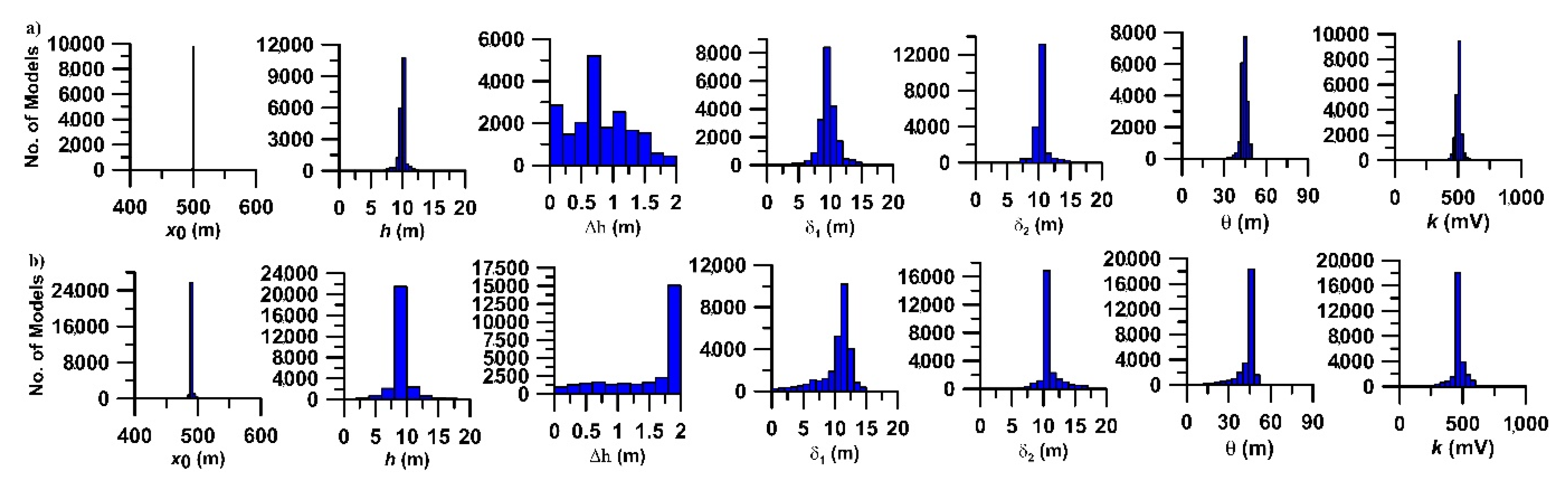
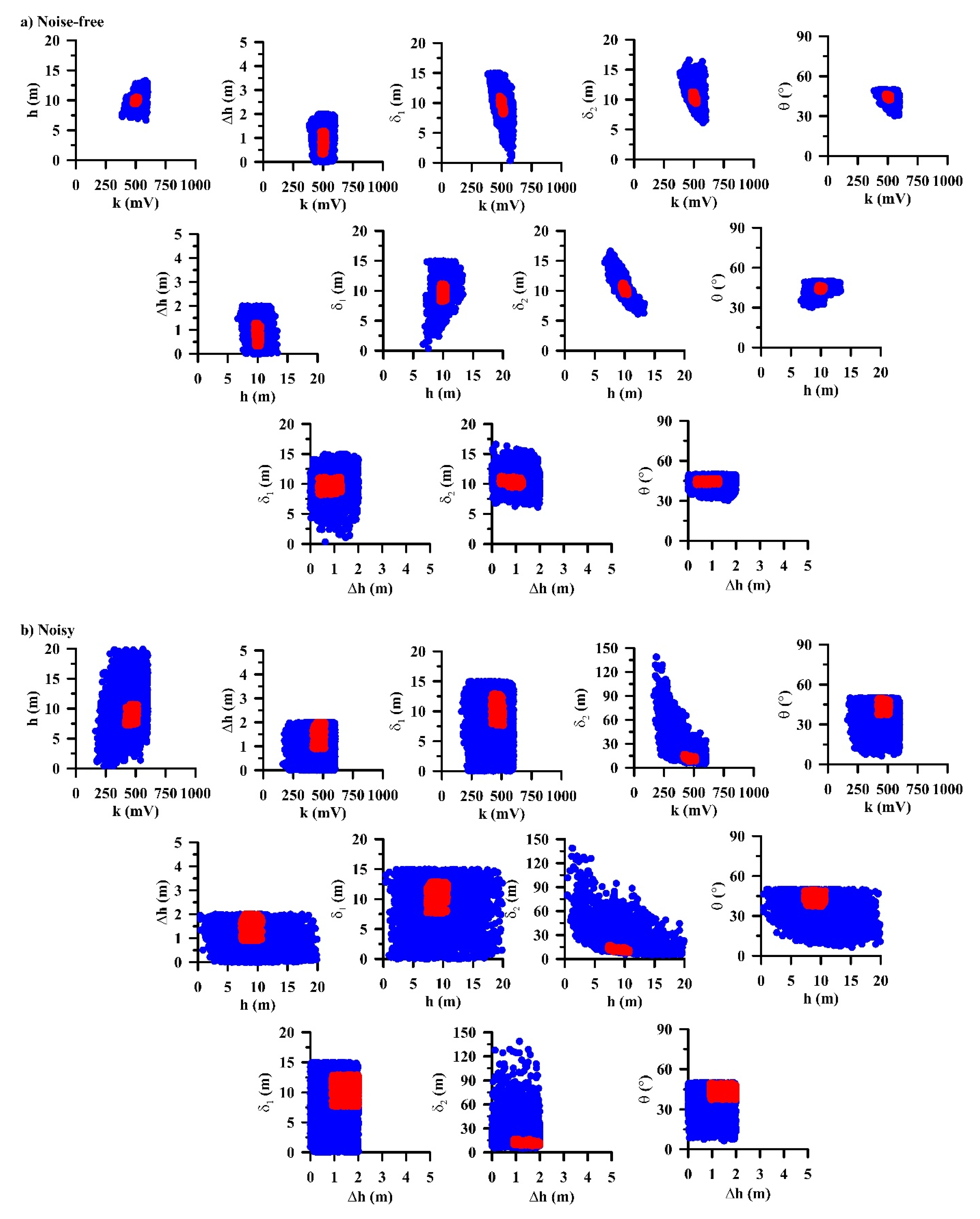
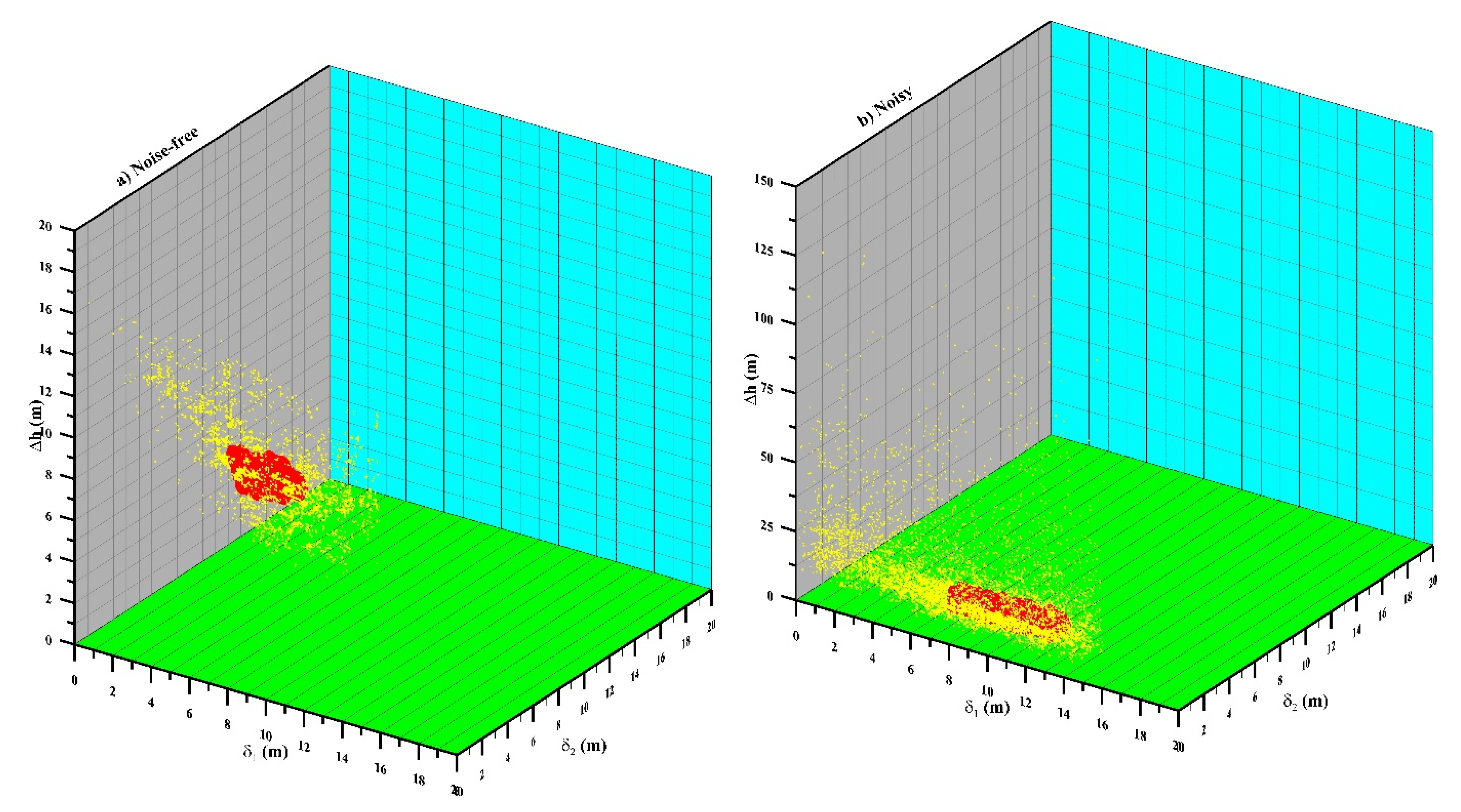
3.1.2. Uncertainty Analysis of Synthetic Models

Uncertainty investigation is always necessary for any geophysical modeling [76]. As a result, a 2D cross-plot was generated for this study to determine the effect of each parameter on the final improved solution, and cross-plots between all the parameters are depicted in Figure 8a. Here, it has been perceived that apart from the parameter Δh; δ₁, δ₂, also indicates a broad solution, and other parameters were well resolved. Still, the parameters for the noise-free data are closer to the actual value (Blue), and the mean model parameters are inside the uncertainty range, which lies in the peak PDF (Red). Figure 8b shows an identical situation from the cross-plots for noise-corrupted data.

Since the cross-plots from the study show that the three parameters Δh, δ₁, and δ₂, depict uncertainty in the interpretation, hence, a 3D cross-plot was also prepared for this investigation (Figure 9). It was found that these three parameters (Δh, δ₁, δ₂) show a diverse solution (yellow) with similar models with smaller errors. The concluding mean model parameter was observed within the well-defined uncertainty margins in the high PDF (Red) region. Figure 9a,b demonstrate the 3D scatter plot for noise-free and noise-corrupted data.

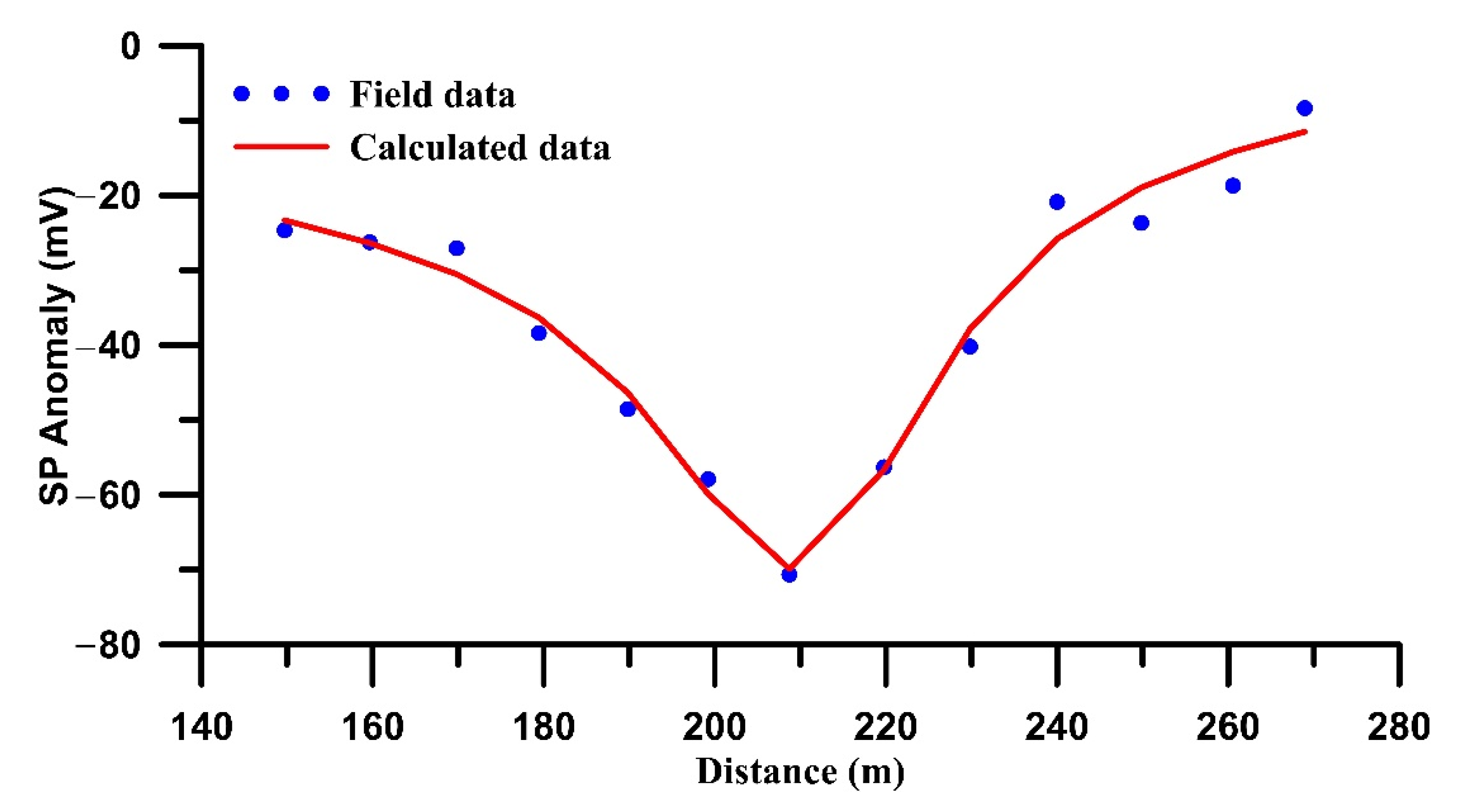
3.2. Self-Potential Anomaly from Real Field Data

To see the robustness of the inversion technique, we have taken three field examples from the published literature [77]. In order to evaluate the accuracy of our inversion results using synthetic data, we have used SP field data for mineral exploration and archaeological investigations. The field data was exactly digitized from the published literature based on the distance (x-axis) and SP anomaly values (y-axis).

3.2.1. Mineral Exploration

The first field example [77] was taken from the polymetallic deposit, Rudnyi Altai, Russia (Figure 10) which is one of the world’s significant volcanogenic massive sulfide deposits [78]. The region is known for its polymetallic sulphide deposits, and the primary components are copper and zinc [79]. Earlier, this field example was analyzed using characteristic points and the tangent method [78], and the interpretation results indicate that the subsurface structure is a thin bed. However, the field example was also taken in this study to decipher the anomaly and the model parameters. It has been seen that the present inversion approach can be able to delineate the SP data. The interpreted parameters, k, x₀, h, Δh, δ₁, δ₂, and θ were found to be 1089.7 mV, 214.8 m, 24.4 m, 61.4 m, 4.2 m, 3.2 m, and 160.6°, respectively. The error estimation for this field data is within the uncertainty limits.

Table 4. Interpretation of the polymetallic deposit, Rudnyi Altai, Russia.

Parameters	Search Limit	Present Study
k (mV)	0–2000	1089.7 ± 144.5
x0 (m)	180–240	214.8 ± 0.9
h (m)	0–30	24.4 ± 2.4
Δh (m)	0–100	61.4 ± 8.7
δ1 (m)	0–10	4.2 ± 0.9
δ2 (m)	0–10	3.2 ± 0.7
θ (°)	0–180	160.6 ± 4.3
error		1.5 × 10−3

shows the inversion results, and Figure 10 shows the field and calculated data.

The second field example [77] was taken from the highly complex terrain of Filizchai polymetallic deposit, Southern Greater Caucasus, Azerbaijan (Figure 11). In fact, ref. [77] also interpreted the field data using the improved characteristic points and the tangent method and inferred it to be a thin bed-type structure. The current technique was also used to analyze the field data, which revealed a thin bed-type structure. The elucidated parameters such as k, x₀, h, Δh, δ₁, δ₂, and θ were found to be 13,261.2 mV, 297.7 m, 40.7 m, 273.4 m, 3.9 m, 11.8 m, and 175°, respectively. The estimated error is found to be low and within uncertainty limits.

Table 5. Interpretation of Filizchai polymetallic deposit, Southern Greater Caucasus, Azerbaijan.

Parameters	Search Limit	Present Study
k (mV)	0–20,000	13,261.2 ± 1550.9
x0 (m)	200–400	297.7 ± 1.7
h (m)	0–100	40.7 ± 3.8
Δh (m)	0–1000	274.3 ± 66.9
δ1 (m)	0–10	3.9 ± 0.8
δ2 (m)	0–20	11.8 ± 2.4
θ (°)	0–180	175.0 ± 1.3
error		9.3 × 10−3

displays the inversion findings, while Figure 11 illustrates the field and computed data.

3.2.2. Archaeological Investigation

The field data was taken from the buried ancient Roman limestone constructions from Halutza, Southern Israel [77], to comprehend the use of SP anomalies from archaeological research (Figure 12). It is renowned for its archaeological strata from different periods [80]. The field data was interpreted by [77] considering thin beds using the quantitative interpretation. The model parameters such as k, x₀, h, Δh, δ₁, δ₂, and θ were found to be 277.6 mV, 4.3 m, 0.7 m, 5.3 m, 1.0 m, 0.5 m, and 110°, respectively. Moreover, ref. [77] estimates the depth and angle to be 0.85 m and 70° (calculated from the opposite side), which closely matches our findings. The error was found to be significantly less and within the uncertainty limits.

Table 6. Interpretation of Archaeological investigation, Halutza, Southern Israel.

Parameters	Search Limit	Present Study	Eppelbaum [78]
k (mV)	0–500	277.6 ± 31.2	-
x0 (m)	0–6	4.3 ± 0.0	-
h (m)	0–10	0.7 ± 0.0	0.85
Δh (m)	0–10	5.3 ± 1.6	-
δ1 (m)	0–5	1.0 ± 0.2	-
δ2 (m)	0–5	0.5 ± 0.1	-
θ (°)	0–180	109.9 ± 3.3	110
error		2.3 × 10−3	-

shows the interpreted results from the inversion, and Figure 12 shows the field and calculated data.

4. Conclusions

The interpretation of Self-Potential anomaly for locating subsurface structures/bodies associated with mineralized zones and its application for archaeological prospection is of enormous importance. SP data have been interpreted considering various subsurface idealized bodies which resemble the subsurface structures. Identifying a dipping layer or a bed is of enormous importance for tracing such bodies. Based on these structures, a very fast simulated annealing (VFSA) global optimization algorithm is used to perform inverse modeling of the Self-Potential (SP) anomalies formed by a two-dimensional dipping layer-like body. Following the objective, model parameters such as amplitude coefficient, depth from the top, origin, vertical sheet thickness, dip angle, and the upper and lower end of the sheet layer of the bodies were interpreted. The inversion technique was then applied to the noise-free synthetic, noisy data in the three field examples of known SP anomalies from Polymetallic deposits of Russia and Azerbaijan, and buried Ancient Roman limestone construction from Halutza, Israel. The results show that it can proficiently interpret all the model parameters with the lowest uncertainty. However, model parameters such as vertical sheet thickness and the upper and lower end of the sheet layer show a large solution. Also, the parameters were found to be within the smallest misfits, and are close to the accurate models with the least uncertainty. Uncertainty analysis from 2D and 3D cross-plot analysis also unveils the same. The present inversion methodology demonstrates that it can provide a reasonable result that is consistent with real field data and previous findings from other interpretation techniques. Hence, it is clear that the inversion algorithm is effective for elucidation of the SP anomalies resulting from the 2D dipping layer with or without a priori geological information.

References

1. Sato, M.; Mooney, H.M. The electrochemical mechanism of sulfide self-potentials. Geophysics 1960, 25, 226–249. [Google Scholar] [CrossRef]
2. Logn, O.; Bolviken, B. Self-potentials at the Joma Pyrite deposit. Geoexploration 1974, 12, 11–28. [Google Scholar] [CrossRef]
3. Corry, C.E. Spontaneous polarization associated with porphyry sulphide mineralization. Geophysics 1985, 50, I020–I034. [Google Scholar] [CrossRef] [Green Version]
4. Wynn, J.C.; Sherwood, S.I. The self-potential (SP) method: An expensive reconnaissance and archaeological mapping tool. J. Field Archaeol. 1984, 11, 195–204. [Google Scholar]
5. Cammarano, F.; Mauriello, P.; Pattella, D.; Piro, S.; Rosso, F.; Versino, L. Integration of high-resolution geophysical methods. Detection of shallow depth bodies of archaeological interest. Ann. Geophys. 1998, 41, 359–368. [Google Scholar] [CrossRef]
6. Eppelbaum, L.V. Advanced Analysis of Self-potential Anomalies: Review of Case Studies from Mining, Archaeology, and Environment. In Self-Potential Method: Theoretical Modeling and Applications in Geosciences; Geophysics Series; Biswas, A., Ed.; Springer: Cham, Switzerland, 2021. [Google Scholar] [CrossRef]
7. Biswas, A. A review on modeling, inversion, and interpretation of self-potential in mineral exploration and tracing paleo-shear zones. Ore Geol. Rev. 2017, 91, 21–56. [Google Scholar] [CrossRef]
8. Kulessa, B.; Hubbard, B.; Brown, G.H. Cross-coupled flow modeling of coincident streaming and electrochemical potentials and application to sub-glacial self-potential data. J. Geophys. Res. 2003, 108, 2381. [Google Scholar] [CrossRef]
9. Jardani, A.; Revil, A.; Boleve, A.; Dupont, J.P. Three-dimensional inversion of self-potential data used to constrain the pattern of groundwater flow in geothermal fields. J. Geophys. Res. Solid Earth 2008, 113, B09204. [Google Scholar] [CrossRef]
10. Mendonca, C.A. Forward and inverse self-potential modeling in mineral exploration. Geophysics 2008, 73, F33–F43. [Google Scholar] [CrossRef]
11. Mehanee, S. An efficient regularized inversion approach for self-potential data interpretation of ore exploration using a mix of logarithmic and non-logarithmic model parameters. Ore Geol. Rev. 2014, 57, 87–115. [Google Scholar] [CrossRef]
12. Mehanee, S. Tracing of paleo-shear zones by self-potential data inversion: Case studies from the KTB, Rittsteig, and Grossensees graphite-bearing fault planes. Earth Planets Space 2015, 67, 14–47. [Google Scholar] [CrossRef]
13. Gobashy, M.; Abdelazeem, M. Metaheuristics Inversion of Self-Potential Anomalies. In Self-Potential Method: Theoretical Modeling and Applications in Geosciences; Geophysics Series; Biswas, A., Ed.; Springer: Cham, Switzerland, 2021. [Google Scholar] [CrossRef]
14. Mehanee, S.; Essa, K.S.; Smith, P.D. A rapid technique for estimating the depth and width of a two-dimensional plate from self-potential data. J. Geophys. Eng. 2011, 8, 447–456. [Google Scholar] [CrossRef]
15. Patella, D. Introduction to ground surface self-potential tomography. Geophys. Prospect. 1997, 45, 653–682. [Google Scholar] [CrossRef]
16. Paul, M.K.; Data, S.; Banerjee, B. Interpretation of SP anomalies due to localized causative bodies. Pure Appl. Geophys. 1965, 61, 95–100. [Google Scholar] [CrossRef]
17. Rao, B.S.R.; Murthy, I.V.R.; Reddy, S.J. Interpretation of self-potential anomalies of some simple geometrical bodies. Pure Appl. Geophys. 1970, 78, 60–77. [Google Scholar] [CrossRef]
18. Roy, S.V.S.; Mohan, N.L. Spectral interpretation of self-potential anomalies of some simple geometric bodies. Pure Appl. Geophys. 1984, 78, 66–77. [Google Scholar]
19. Murthy, B.V.S.; Haricharan, P. Nomograms for the complete interpretation of spontaneous potential profiles over sheet like and cylindrical 2D structures. Geophysics 1985, 50, 1127–1135. [Google Scholar] [CrossRef]
20. Abdelrahman, E.M.; Sharafeldin, M.S. A least-squares approach to depth determination from self-potential anomalies caused by horizontal cylinders and spheres. Geophysics 1997, 62, 44–48. [Google Scholar] [CrossRef]
21. Tlas, M.; Asfahani, J. A best-estimate approach for determining self-potential parameters related to simple geometric shaped structures. Pure Appl. Geophys. 2007, 164, 2313–2328. [Google Scholar] [CrossRef]
22. Essa, K.; Mahanee, S.; Smith, P.D. A new inversion algorithm for estimating the best fitting parameters of some geometrically simple body to measured self-potential anomalies. Explor. Geophys. 2008, 39, 155–163. [Google Scholar] [CrossRef]
23. Göktürkler, G.; Balkaya, Ç. Inversion of self-potential anomalies caused by simple geometry bodies using global optimization algorithms. J. Geophys. Eng. 2012, 9, 498–507. [Google Scholar] [CrossRef]
24. Tlas, M.; Asfahani, J. An approach for interpretation of self-potential anomalies due to simple geometrical structures using flair function minimization. Pure Appl. Geophys. 2013, 170, 895–905. [Google Scholar] [CrossRef]
25. Biswas, A.; Sharma, S.P. Interpretation of self-potential anomaly over idealized body and analysis of ambiguity using very fast simulated annealing global optimization. Near Surf. Geophys. 2015, 13, 179–195. [Google Scholar] [CrossRef]
26. Roudsari, M.S.; Beitollahi, A. Laboratory modelling of self-potential anomalies due to spherical bodies. Explor. Geophys. 2015, 46, 320–331. [Google Scholar] [CrossRef]
27. Di Maio, R.; Rani, P.; Piegari, E.; Milano, L. Self-potential data inversion through a Genetic-Price algorithm. Comput. Geosci. 2016, 94, 86–95. [Google Scholar] [CrossRef]
28. Di Maio, R.; Piegari, E.; Rani, P.; Avella, A. Self-Potential data inversion through the integration of spectral analysis and tomographic approaches. Geophys. J. Int. 2016, 206, 1204–1220. [Google Scholar] [CrossRef]
29. Abdelrahman, E.M.; Abdelazeem, M.; Gobashy, M. A minimization approach to depth and shape determination of mineralized zones from potential field data using the Nelder-Mead simplex algorithm. Ore Geol. Rev. 2019, 114, 103123. [Google Scholar] [CrossRef]
30. Abdelazeem, M.; Gobashy, M.; Khalil, M.H.; Abdraboub, M. A complete model parameter optimization from self-potential data using Whale algorithm. J. Appl. Geophys. 2019, 170, 103825. [Google Scholar] [CrossRef]
31. Paul, M.K. Direct interpretation of self-potential anomalies caused by inclined sheets of infinite extension. Geophysics 1965, 30, 418–423. [Google Scholar] [CrossRef]
32. Jagannadha, R.S.; Rama, R.P.; Radhakrishna, M.I.V. Automatic inversion of self-potential anomalies of sheet-like bodies. Comput. Geosci. 1993, 19, 61–73. [Google Scholar] [CrossRef]
33. Rao, A.D.; Babu, H.; Sivakumar Sinha, G.D. A Fourier transform method for the interpretation of self-potential anomalies due to two-dimensional inclined sheet of finite depth extent. Pure Appl. Geophys. 1982, 120, 365–374. [Google Scholar] [CrossRef]
34. Sundararajan, N.; Arun Kumar, I.; Mohan, N.L.; Seshagiri-Rao, S.V. Use of Hilbert transform to interpret self-potential anomalies due to two dimensional inclined sheets. Pure Appl. Geophys. 1990, 133, 117–126. [Google Scholar] [CrossRef]
35. Sundararajan, N.; Srinivasa Rao, P.; Sunitha, V. An analytical method to interpret self-potential anomalies caused by 2D inclined sheets. Geophysics 1998, 63, 1551–1555. [Google Scholar] [CrossRef]
36. Murthy, I.V.R.; Sudhakar, K.S.; Rao, P.R. A new method of interpreting self- potential anomalies of two-dimensional inclined sheets. Comput. Geosci. 2005, 31, 661–665. [Google Scholar] [CrossRef]
37. Abdelrahman, E.M.; El-Araby, H.M.; Hassanein, A.G.; Hafez, M.A. New methods for shape and depth determinations from SP data. Geophysics 2003, 68, 1202–1210. [Google Scholar] [CrossRef] [Green Version]
38. El-Kaliouby, H.M.; Al-Garani, M.A. Inversion of self-potential anomalies caused by 2D inclined sheets using neural networks. J. Geophys. Eng. 2009, 6, 29–34. [Google Scholar] [CrossRef] [Green Version]
39. Monteiro Santos, F.A. Inversion of Self-potential of Idealized bodies anomalies using particle swarm optimization. Comput. Geosci. 2010, 36, 1185–1190. [Google Scholar] [CrossRef]
40. Essa, K.S. A new algorithm for gravity or self-potential data interpretation. J. Geophys. Eng. 2011, 8, 434–446. [Google Scholar] [CrossRef]
41. Dmitriev, A.N. Forward and inverse self-potential modeling: A new approach. Russ. Geol. Geophys. 2012, 53, 611–622. [Google Scholar] [CrossRef]
42. Sharma, S.P.; Biswas, A. Interpretation of self-potential anomaly over 2D inclined structure using very fast simulated annealing global optimization—An insight about ambiguity. Geophysics 2013, 78, WB3–WB15. [Google Scholar] [CrossRef]
43. Roudsari, M.S.; Beitollahi, A. Forward modeling and inversion of self-potential anomalies caused by 2D inclined sheets. Explor. Geophys. 2013, 44, 176–184. [Google Scholar] [CrossRef]
44. Biswas, A.; Sharma, S.P. Resolution of multiple sheet-type structures in self-potential measurement. J. Earth Syst. Sci. 2014, 123, 809–825. [Google Scholar] [CrossRef] [Green Version]
45. Biswas, A.; Sharma, S.P. Optimization of Self-Potential interpretation of 2-D inclined sheet-type structures based on Very Fast Simulated Annealing and analysis of ambiguity. J. Appl. Geophys. 2014, 105, 235–247. [Google Scholar] [CrossRef]
46. Biswas, A. A comparative performance of Least Square method and Very Fast Simulated Annealing Global Optimization method for interpretation of Self-Potential anomaly over 2-D inclined sheet type structure. J. Geol. Soc. India 2016, 88, 493–502. [Google Scholar] [CrossRef]
47. Biswas, A.; Sharma, S.P. Interpretation of Self-potential anomaly over 2-D inclined thick sheet structures and analysis of uncertainty using very fast simulated annealing global optimization. Acta Geod. Geophys. 2017, 52, 439–455. [Google Scholar] [CrossRef] [Green Version]
48. Biswas, A. Inversion of amplitude from the 2-D analytic signal of self-potential anomalies. In Minerals; Essa, K., Ed.; InTech Education and Publishing: London, UK, 2019; pp. 13–45. [Google Scholar]
49. Hafez, M.A. Interpretation of the self-potential anomaly over a 2D inclined plate using a moving average window curves method. J. Geophys. Eng. 2005, 2, 97–102. [Google Scholar] [CrossRef]
50. Essa, K.S.; El-Hussein, M. A new approach for the interpretation of self-potential data by 2-D inclined plate. J. Appl. Geophys. 2017, 136, 455–461. [Google Scholar] [CrossRef]
51. Rao, K.; Jain, S.; Biswas, A. Global Optimization for Delineation of Self-potential Anomaly of a 2D Inclined Plate. Nat. Resour. Res. 2021, 30, 175–189. [Google Scholar] [CrossRef]
52. Meiser, P. A method of quantitative interpretation of self-potential measurements. Geophys. Prospect. 1962, 10, 203–218. [Google Scholar] [CrossRef]
53. Murthy, B.V.S.; Haricharan, P. Self-potential anomaly over double line of poles—Interpretation through log curves. Proc. Indian Acad. Sci. (Earth Planet. Sci.) 1984, 93, 437–445. [Google Scholar] [CrossRef]
54. Abdelrahman, E.M.; Saber, H.S.; Essa, K.S.; Fouad, M.A. A least-squares approach to depth determination from numerical horizontal self-potential gradients. Pure Appl. Geophys. 2004, 161, 399–411. [Google Scholar] [CrossRef]
55. El-Araby, H.M. A new method for complete quantitative interpretation of self-potential anomalies. J. Appl. Geophys. 2004, 55, 211–224. [Google Scholar] [CrossRef]
56. Ben, U.C.; Ekwok, S.E.; Akpan, A.E.; Mbonu, C.C. Interpretation of magnetic anomalies by simple geometrical structures using the manta-ray foraging optimization. Front. Earth Sci. 2022, 10, 849079. [Google Scholar] [CrossRef]
57. Essa, K.S.; Diab, Z.E. Magnetic data interpretation for 2D dikes by the metaheuristic bat algorithm: Sustainable development cases. Sci. Rep. 2022, 12, 14206. [Google Scholar] [CrossRef]
58. Peksken, E.; Yas, T.; Kayman, A.Y.; Ozkan, C. Application of particle swarm optimization on self-potential data. J. Appl. Geophys. 2011, 75, 305–318. [Google Scholar] [CrossRef]
59. Li, X.; Yin, M. Application of differential evolution algorithm on self-potential data. PLoS ONE 2012, 7, e51199. [Google Scholar] [CrossRef]
60. Balkaya, C. An implementation of differential evolution algorithm for inversion of geoelectrical data. J. Appl. Geophys. 2013, 98, 160–175. [Google Scholar] [CrossRef]
61. Cui, Y.; Zhu, X.; Chen, Z. Performance evaluation for intelligent optimization algorithms in self-potential data inversion. J. Cent. S. Univ. 2016, 23, 2659–2668. [Google Scholar] [CrossRef]
62. Sungkono; Warnana, D.D. Black hole algorithm for determining model parameter in self-potential data. J. Appl. Geophys. 2018, 148, 189–200. [Google Scholar] [CrossRef]
63. Sungkono. An efficient global optimization method for self-potential data inversion using micro-differential evolution. J. Earth Syst. Sci. 2020, 129, 178. [Google Scholar] [CrossRef]
64. Biswas, A. Identification and Resolution of Ambiguities in Interpretation of Self-Potential Data: Analysis and Integrated Study around South Purulia Shear Zone, India. Ph.D. Thesis, Department of Geology and Geophysics, Indian Institute of Technology Kharagpur, Kharagpur, India, 2013. [Google Scholar]
65. Biswas, A.; Sharma, S.P. Integrated geophysical studies to elicit the structure associated with Uranium mineralization around South Purulia Shear Zone, India: A Review. Ore Geol. Rev. 2016, 72, 1307–1326. [Google Scholar] [CrossRef]
66. Eppelbaum, L.V. Quantitative interpretation of magnetic anomalies from bodies approximated by thick bed models in complex environments. Environ. Earth Sci. 2015, 74, 5971–5988. [Google Scholar] [CrossRef]
67. Biswas, A. Self-Potential Method: Theoretical Modeling and Applications in Geosciences; Geophysics Series; Springer International Publishing: Cham, Switzerland, 2021; Volume X, 314p, ISBN 978-3-030-79332-6. [Google Scholar] [CrossRef]
68. Sen, M.K.; Stoffa, P.L. Global Optimization Methods in Geophysical Inversion, 2nd ed.; Cambridge University Press: London, UK, 2013; 289p. [Google Scholar]
69. Biswas, A. Interpretation of residual gravity anomaly caused by a simple shaped body using very fast simulated annealing global optimization. Geosci. Front. 2015, 6, 875–893. [Google Scholar] [CrossRef] [Green Version]
70. Biswas, A. Interpretation of gravity anomaly over 2D vertical and horizontal thin sheet with finite length and width. Acta Geophys. 2020, 68, 1083–1096. [Google Scholar] [CrossRef]
71. Mosegaard, K.; Tarantola, A. Monte Carlo sampling of solutions to inverse problems. J. Geophys. Res. 1995, 100, 12431–12447. [Google Scholar] [CrossRef]
72. Sen, M.K.; Stoffa, P.L. Bayesian inference, Gibbs sampler and uncertainty estimation in geophysical inversion. Geophys. Prospect. 1996, 44, 313–350. [Google Scholar] [CrossRef]
73. Biswas, A.; Parija, M.P.; Kumar, S. Global nonlinear optimization for the interpretation of source parameters from total gradient of gravity and magnetic anomalies caused by thin dyke. Ann. Geophys. 2017, 60, G0218. [Google Scholar] [CrossRef] [Green Version]
74. Biswas, A. Inversion of source parameters from magnetic anomalies for mineral/ore deposits exploration using global optimization technique and analysis of uncertainty. Nat. Resour. Res. 2018, 27, 77–107. [Google Scholar] [CrossRef]
75. Trivedi, S.; Kumar, P.; Parija, M.P.; Biswas, A. Global Optimization of Model Parameters from the 2-D Analytic Signal of Gravity and Magnetic anomalies 2020. In Advances in Modeling and Interpretation in Near Surface Geophysics; Biswas, A., Sharma, S.P., Eds.; Springer: Cham, Switzerland, 2020; pp. 189–221. [Google Scholar]
76. Daviran, M.; Parsa, M.; Maghsoudi, A.; Ghezelbash, R. Quantifying Uncertainties Linked to the Diversity of Mathematical Frameworks in Knowledge-Driven Mineral Prospectivity Mapping. Nat. Resour. Res. 2022, 31, 2271–2287. [Google Scholar] [CrossRef]
77. Eppelbaum, L.V. Review of Processing and Interpretation of Self-Potential Anomalies: Transfer of Methodologies Developed in Magnetic Prospecting. Geosciences 2021, 11, 194. [Google Scholar] [CrossRef]
78. Eremin, N.I.; Dergachev, A.L.; Sergeeva, N.E. Rudny Altay in comparison with the other largest sulfide provinces of the world. In Greater Altay as a Unique Rare Metal-Gold-Polymetallic Province of Central Asia: Proceedings of the International Conference; East Kazakhstan State Technical University Publishing: Ust-Kamenogorsk, Kazakhstan, 2010; pp. 91–92. (In Russian) [Google Scholar]
79. Lobanov, K.; Yakubchuk, A.; Creaser, R.A. Besshi-type VMS deposits of the Rudny Altai (Central Asia). Econ. Geol. 2014, 109, 1403–1430. [Google Scholar] [CrossRef]
80. Reich, R. Architecture of Ancient Israel; Israel Exploration Society: Jerusalem, Israel, 1992. [Google Scholar]
Figure 1. The source geometry for the 2D dipping layer/bed.
Minerals 12 01484 g001
Figure 2. Flowchart of the VFSA algorithm to interpret SP data [51].
Minerals 12 01484 g002
Figure 3. Convergence for all parameters and the misfit.
Minerals 12 01484 g003
Figure 4. Histogram for Model 1: (a) Noise-free and (b) Noisy synthetic data.
Minerals 12 01484 g004
Figure 5. Fits for Model 1: (a) Noise-free and (b) Noisy synthetic data.
Minerals 12 01484 g005
Figure 6. Histogram for Model 2: (a) Noise-free and (b) Noisy synthetic data.
Minerals 12 01484 g006
Figure 7. Fits for Model 2: (a) Noise-free and (b) Noisy synthetic data.
Minerals 12 01484 g007
Figure 8. 2D cross-plot for layer/bed Model 1: (a) Noise-free, and (b) Noisy synthetic data.
Minerals 12 01484 g008
Figure 9. 3D cross-plot for 2D layer/bed Model 1: (a) Noise-free, and (b) Noisy synthetic data.
Minerals 12 01484 g009
Figure 10. Fits for field data of polymetallic deposit, Rudnyi Altai, Russia.
Minerals 12 01484 g010
Figure 11. Fits for field data of Filizchai polymetallic deposit, Southern Greater Caucasus, Azerbaijan.
Minerals 12 01484 g011
Figure 12. Fits for field data of Archaeological investigation, Halutza, Southern Israel.
Minerals 12 01484 g012