Modelling Bubble Flow Hydrodynamics: Drift-Flux and Molerus Models

Abstract

Minerals flotation is a widely used process to produce base metal concentrates through the selective capture of particles on the surface of bubbles. The process performance depends on the size distribution of the bubble population generated by gas dispersion, which is characterized by three variables: superficial gas velocity, gas holdup, and bubble size. A literature review revealed that current instrumentation cannot provide reliable on-line measurement of these variables except for gas velocity. There are some promising alternatives for gas holdup, but bubble size measurement will continue to be unavailable. The use of a model that integrates the three gas dispersion variables makes possible the calculation of one of the variables when knowing the values of the other two. Modelling bubble flow has been pursued using two approaches: determining the bubble terminal velocity reduction by the presence of other bubbles and regarding the bubble swarm as a packed bed through which a fluid is allowed to flow. Models based on these approaches (drift-flux and Molerus, respectively) were found in the literature and used to assess their prediction ability. Gas holdup predictions for known values of gas velocity and bubble size showed similar trends for both models; Molerus results were always higher than those obtained with the drift-flux model, and the difference between both predictions increased with bubble size and gas velocity. A relationship between bubble surface area flux and gas holdup was explored (a single line was expected); Molerus values showed a noticeable effect of bubble size, while drift-flux results showed a minor effect of bubble size only for gas holdups below 10%. Model accuracy was established using a data set collected to characterize frother roles in flotation for six commercial frothers, which included values of the three gas dispersion variables measured simultaneously and reported at the same conditions. The results indicate that bubble size predictions obtained from Molerus model are closer to the measured values than those obtained from the drift-flux model. Drift-flux predictions systematically underestimated the measured bubble size, with relative errors between 10 and 30%, while Molerus predictions showed values around the measured size with relative errors not larger than 15% (and in most cases below 10%). The accuracy of the Molerus predictions is acceptable for applications in the control of individual cells and flotation circuits operation. Further testing to assess the performance of Molerus model with data collected in lab and industrial mechanical cells and columns, where conditions in the test volume may not be stable or homogeneous, is recommended.

1. Introduction

Minerals flotation, a widely used process to selectively separate particles of a valuable mineral based on its hydrophobicity, involves the formation and separation of bubble–particle aggregates (bubbles with collected particles on their surfaces). The formation of bubble–particle aggregates occurs in a collection zone as the result of collisions between rising bubbles and hydrophobic mineral particles suspended or sedimenting in a liquid medium. These conditions are created in mechanical cells and columns by continuous generation of bubble swarms at the bottom of large tanks filled with mineral pulps, using a variety of rotor–stator combinations in the case of mechanical cells and, in the case of columns, by injection of gas or air–pulp mixtures after high-intensity contact.

The efficiency of the process relies heavily on the size and liberation characteristics of the particle population formed at the ore-grinding stage and on the external bubble surface area generated by gas dispersion in the collection zone, which is defined by the resulting bubble size distribution. Gas dispersion technologies are operated to form bubbles with the smallest possible size, which means the largest interfacial areas to boost particle collection. Because of the high bubble concentration and intense turbulence in the region where bubbles are formed, a high bubble collision frequency is inevitable, which leads to coalescence with significant bubble size increases unless the formation bubble size is preserved by addition of frothers and/or by the presence of soluble inorganic salts in the liquid medium. Surfactants molecules and inorganic ions adsorb on the bubble surface, forming a protective layer that reduces or eliminates the coalescence of colliding bubbles and affects its rising velocity [1]. Increasing frother or salt concentrations decreases bubble size until a value is reached (critical coalescence concentration CCC), beyond which bubble size is not further reduced. The CCC, which is not considered a physical property of the frother or inorganic salt, depends on the machine and the operating conditions used during its measurement.

Bubble flow hydrodynamics and flotation machine performance are defined by the number, size, and velocity of the bubbles generated in the collection zone. These parameters are intrinsically related; after a gas flowrate is dispersed into a bubble population with a known size distribution, the number of bubbles is established, and a gas holdup develops as the bubbles rise and reach a stable velocity. The superficial gas velocity is the control variable that defines for any gas dispersion technology the characteristics of the generated bubble population, and once selected, the bubble size distribution and corresponding gas holdup cannot be independently modified.

Three parameters (gas dispersion variables) are used to characterize the flow of rising bubbles in the collection zone of flotation machines: the superficial gas velocity J_g (volumetric gas flowrate per unit of cross-sectional area of the machine); the bubble size D_b (a calculated average from a bubble size distribution); and the gas holdup ε_g (volumetric fraction of gas in the aerated collection-zone pulp). The performance of flotation circuits depends on cell operating strategies based on the control of interfacial areas and particle residence times, which require calculations with known values of the gas dispersion variables.

Sensors and techniques for off-line measurement of these variables in laboratory and industrial machines have been developed and demonstrated [2,3,4,5,6,7,8,9,10]. Although gas dispersion measurements have been successfully used to diagnose the operation and performance of laboratory and industrial units [11,12], applications driving machine operation and circuit optimization efforts have not occurred because on-line techniques for measuring bubble size and gas holdup are unavailable. A literature search revealed that continuous measurement of bubble size in industrial flotation machines is not possible with the current instrumentation, but in the case of gas holdup, some promising alternatives have been proposed and successfully tested [13,14,15,16].

Although the availability of a reliable technique for on-line gas holdup measurement would be a significant advance in mineral flotation technology, missing bubble size measurement will continue to be a major limitation. A possible answer is the use of a model, given the close relationship between the gas dispersion variables, that makes possible the calculation of one of them when knowing the values of the other two. Applications of this approach to calculate bubble sizes from gas velocity and holdup values have been reported in the literature [17,18,19,20]. Model development for the flow of bubbles has been limited because of the difficulties in generating a continuous flow of single-size bubbles and the problems derived in the interpretation of results that require consideration of the effect of frothers and ions of inorganic salts. However, because of the similarities between the forces driving a rising bubble and a sedimenting particle, models that include equations derived for the movement of solid spheres and particles have been proposed.

A literature search for a model that can be used to reliably predict bubble sizes from gas velocity and holdup measurements was undertaken. It was found that hydrodynamic modelling of bubble flows has been developed using two approaches: characterizing the reduction of bubble rising velocities by the presence of other bubbles and regarding the suspension as a packed bed through which a fluid is allowed to flow [21,22,23]. Two models were selected to test their prediction’s ability: the drift-flux model based on the first approach and the model proposed by Molerus based on the second approach [24]. Both models are described, and calculations are demonstrated for a range of conditions of interest in flotation. The prediction accuracy was assessed using a set of data obtained in the CCC determination for several frothers in a laboratory flotation column; this data set includes measurements of the three gas dispersion variables simultaneously measured and corrected to the same conditions of pressure and temperature.

2. Drift-Flux Model

A separated-flow model based on drift flux analysis [25] has been used in flotation for characterizing the flow of a dispersed gas phase, in the form of a bubble swarm, through a side-by-side flowing liquid phase. The drift flux represents the volumetric flux of the gas or liquid phase relative to an observer moving at the average bubble velocity (slip velocity U_bs). The slip velocity, which is a function of bubble size, is calculated using the following equation:

$${\mathrm{U}}_{\mathrm{bs}}=\frac{{\mathrm{J}}_{\mathrm{g}}}{{\mathsf{\epsilon }}_{\mathrm{g}}}+\frac{{\mathrm{J}}_{\mathrm{l}}}{{\mathsf{\epsilon }}_{\mathrm{l}}}=\frac{{\mathrm{J}}_{\mathrm{g}}}{{\mathsf{\epsilon }}_{\mathrm{g}}}+\frac{{\mathrm{J}}_{\mathrm{l}}}{{1-\mathsf{\epsilon }}_{\mathrm{g}}}$$

(1)

where J_g and J_l are the gas and liquid superficial velocities, respectively, and ε_g and ε_l are the gas and liquid holdups, respectively. This equation (drift flux equation) applies to co-current and counter-current flows of gas and liquid. It is considered that flows and forces opposing gravity, i.e., in the direction of freely moving bubbles, are positive.

Bubbles rise in a water solution due to the action of three forces: two static (weight F_g and buoyancy F_b) and one proportional to the rising velocity relative to the fluid (friction or drag force F_k). The static forces oppose each other, are vertical, and constant as depend on the bubble volume and not its shape. Buoyancy, the weight of solution displaced by the bubble, is larger than the weight of the volume of gas forming the bubble because of its higher density, which results in a difference between the static forces that drives bubbles to rise:

$${\mathrm{F}}_{\mathrm{b}}{-\mathrm{F}}_{\mathrm{g}}={\mathrm{gV}}_{\mathrm{b}}\left({\mathsf{\rho }}_{\mathrm{l}}{-\mathsf{\rho }}_{\mathrm{g}}\right)$$

(2)

V_b is the volume of the bubble, g is the acceleration of gravity, and ρ_l and ρ_g are the densities of the liquid solution and gas, respectively.

The friction force opposes movement, and it is a strong function of the slip velocity. As the bubbles rise, a point is reached where the summation of the three forces is zero, and a steady terminal velocity is achieved (Ut). The calculation of the terminal velocity requires a value for the friction force. Theoretical calculation of the friction force is complex; the only theoretical derivation of the friction force has been that performed by Stokes in 1851 (as reported in [26]), for the simple case of creeping flow around a single, small, spherical particle in an infinite fluid, but its application range is out of that relevant in flotation.

No other theoretical treatment has been developed for a particle or bubble moving faster (higher Re), for a non-spherical particle or bubble, or for situations when there is interference between particles. However, the problem has been widely examined experimentally. The results were interpreted utilizing concepts borrowed from the characterization of friction losses for the flow of liquids in pipes to obtain a relationship for calculation of the friction force:

$${\mathrm{F}}_{\mathrm{k}}=\frac{{\mathrm{C}}_{\mathrm{d}}{\mathrm{A}}_{\mathrm{x}}{\mathsf{\rho }}_{\mathrm{l}}{\mathrm{U}}_{\mathrm{t}}^2}{2}$$

(3)

where C_d is a drag coefficient, and A_x is the projected area of the particle or bubble in the direction of the flow; for a spherical bubble of diameter d_b, A_x is the area of a circle of diameter d_b.

The following expression is obtained for calculating the terminal velocity of a spherical particle or bubble when the summation of forces is zero (Equation (2) equal to (3)):

$${\mathrm{U}}_{\mathrm{t}}=\sqrt{\frac{4\mathrm{g}\left({\mathsf{\rho }}_{\mathrm{l}} {-\mathsf{\rho }}_{\mathrm{g}}\right){\mathrm{d}}_{\mathrm{b}}}{{3\mathsf{\rho }}_{\mathrm{l}}{\mathrm{C}}_{\mathrm{d}}}}$$

(4)

The calculation requires a value for the drag coefficient. The literature contains numerous correlations to estimate C_d that have been developed almost exclusively for the sedimentation of solid spheres and particles. Measurements involving the flow of bubble swarms have been limited because of the difficulties to generate a continuous flow of single-size bubbles, and of the problems derived in the interpretation of results that require consideration of the effect of frothers and ions of inorganic salts. Bubble shapes and velocities are affected by the presence of surface-active agents in the solution, which adsorb on the surface of bubbles affecting its rigidity [27,28,29,30]; this is not the case for solid spheres and particles.

Drag coefficients are often reported using dimensionless numbers that include values of physical properties of the phases involved and of operating conditions. A correlation frequently used in flotation applications [18,20,31,32], has been that proposed by Schiller and Nauman (as reported in [26]), which, although developed for the sedimentation of single steel spheres with Reynolds numbers up to 800, has been applied to rising single bubbles:

$${\mathrm{C}}_{\mathrm{d}}=\frac{24}{{\mathrm{Re}}_{\mathrm{b}}}\left[1+0.15{\mathrm{Re}}_{\mathrm{b}}^{0.687}\right]{\hspace{1em}\mathrm{Re}}_{\mathrm{b}}<800$$

(5)

The dimensionless Reynolds number (Re_b) is calculated using the terminal velocity of a single bubble rising in a liquid medium with the same characteristics as that where the bubble swarm is flowing:

$${\mathrm{Re}}_{\mathrm{b}}=\frac{{\mathsf{\rho }}_{\mathrm{l}}{\mathrm{U}}_{\mathrm{t}}{\mathrm{d}}_{\mathrm{b}}}{{\mathsf{\mu }}_{\mathrm{l}}}$$

(6)

where μ_l is the dynamic viscosity of the liquid medium.

A combination of Equations (4)–(6) results in an expression to calculate bubble terminal velocity if the bubble size is known:

$${\mathrm{U}}_{\mathrm{t}}=\frac{{\mathrm{g}(\mathsf{\rho }}_{\mathrm{l}}{-\mathsf{\rho }}_{\mathrm{g}}{)\mathrm{d}}_{\mathrm{b}}^2}{{18\mathsf{\mu }}_{\mathrm{l}}\left[1+{0.15\mathrm{Re}}_{\mathrm{b}}^{0.687}\right]}$$

(7)

Calculation of the drift velocity (Equation (1)) and of the terminal velocity (Equation (7)) makes possible the estimation of bubble size for a bubble swarm based on the pioneering work of Richardson and Zaki [22], which has been fundamental in the development of the drift-flux model. Results of measurements of the settling rate of uniformly sized spherical particles larger than 100 μm, as a function of particle concentration, demonstrated that the ratio of the sedimentation to the terminal velocity is related by a function of the gas holdup that accounts for the reduction of the terminal velocity by interactions with other particles:

$$\frac{{\mathrm{U}}_{\mathrm{bs}}}{{\mathrm{U}}_{\mathrm{t}}}={(1-{\mathsf{\epsilon }}_{\mathrm{g}})}^{\mathrm{m}-1}$$

(8)

The exponent m is calculated from

$$\mathrm{m}=\left(4.45+18\frac{{\mathrm{d}}_{\mathrm{b}}}{{\mathrm{D}}_{\mathrm{c}}}\right){\mathrm{Re}}_{\mathrm{b}}^{-0.1}\hspace{1em}\hspace{1em}1<{\mathrm{Re}}_{\mathrm{b}}\le 200$$

(9)

$$\mathrm{m}={4.45\mathrm{Re}}_{\mathrm{b}}^{-0.1}\hspace{1em}\hspace{1em}\hspace{1em}200<{\mathrm{Re}}_{\mathrm{b}}\le 500$$

(10)

$$\mathrm{m}=2.39\hspace{1em}\hspace{1em}500<{\mathrm{Re}}^{\mathrm{b}}$$

(11)

where D_C is the diameter of the cell or column.

Bubble size prediction is basically a search for the size of a bubble with a terminal velocity that, after correction for the interaction with surrounding bubbles, is equal to the measured slip velocity calculated from the known values of gas holdup and the gas and liquid superficial velocities (Equation (1)). The solution requires two iterative procedures: one initiated by assumption of a bubble size and then searching for the Re number that gives the same terminal velocity from Equations (6) and (7), followed by calculation of exponent m (Equations (9)–(11)) and bubble size using Equation (7); this calculation sequence is repeated until the assumed and calculated bubble sizes are the same.

It is important to point out that the model requires drag coefficients to determine the terminal velocity of bubbles. There are many equations in the literature developed to calculate drag coefficients for the settling of solid spheres and particles and, in most cases, in water solutions with no addition of frother and soluble inorganic salts (i.e., Equation (5) used in this work). Richardson and Zaki’s equation (Equation (8)) requires swarm and terminal velocities obtained in the same liquid medium, which is a major limitation for the selection of a drag coefficient equation. This is even more challenging when the model is applied to bubbles rising in mineral pulps.

3. Molerus’ Model

Fixed beds and particulate fluidized beds are similar physical processes. Equations to calculate pressure drop and particle drag in fixed beds can be easily extended to particulate fluidized beds at low fluid flowrates, which is the case of bubble columns operating under a uniform bubbling regime. As particles are homogeneously distributed, the total bed can be considered as the stacking of individual cells. The cell model considered divides the bed in as many cells as individual particles, each with a surrounding pore space around the particle for the fluid to flow, which is characterized by a length ratio (r₀/δ) parameter [24]. This parameter relates the characteristic dimension of the particles (r₀), not necessarily spheres, to that of the pores (δ), and it is a function of the gas holdup and a packing parameter ς determined by calibration:

$$\frac{{\mathrm{r}}_0}{\mathsf{\delta }}=\frac{1}{(\mathsf{\varsigma }/\sqrt[3]{{\mathsf{\epsilon }}_{\mathrm{g}}}-1)}$$

(12)

The estimation of the dependence of a particle drag on the packing characteristics of a fixed bed, at different Reynolds numbers, result in the following empirical formula [24]:

$$\mathrm{Eu}=\frac{24}{\mathrm{Re}}\left[{1+\mathrm{K}}_1\left\{\frac{{\mathrm{r}}_0}{\mathsf{\delta }}+\frac{1}{2}{\left(\frac{{\mathrm{r}}_0}{\mathsf{\delta }}\right)}^2\right\}\right]+\frac{4}{\sqrt{\mathrm{Re}}}\left[{1+\mathrm{K}}_2{\left(\frac{{\mathrm{r}}_0}{\mathsf{\delta }}\right)}^{1.5}\right]+\left[0.4+\frac{{\mathrm{K}}_3}{{\mathrm{Re}}^{\mathrm{n}}}\left(\frac{{\mathrm{r}}_0}{\mathsf{\delta }}\right)\right]$$

(13)

where K₁, K₂, K₃, and n are constants to be determined by calibration, and Eu is the Euler number for fluidization:

$$\mathrm{Eu}=\frac{4\mathrm{g}\left({\mathsf{\rho }}_{\mathrm{l}}{-\mathsf{\rho }}_{\mathrm{g}}\right){\mathrm{d}}_{\mathrm{b}}}{{3\mathsf{\rho }}_{\mathrm{l}}{\mathrm{U}}^2}{\mathsf{\epsilon }}^2$$

(14)

Calibration of Equation (13) using bed expansion values measured in the fluidization of solid particles by Wilhelm and Kwauk [33] and by Wild, as reported by Molerus [24], resulted in the following values for the parameters involved: K₁ = 0.341, K₂ = 0.07, K₃ = 0.907, n = 0.1, and ς = 0.9. Introducing the parameter-calibrated values and replacing the Euler number by the dimensionless bubble size β, the following equation is obtained [24]:

$${\mathsf{\beta }}^3=18\left[1+0.341\left\{\frac{r_0}{\mathsf{\delta }}+\frac{1}{2} {\left(\frac{r_0}{\mathsf{\delta }}\right)}^2\right\}\right]\mathrm{Re}+3\left[1+0.07{\left(\frac{{\mathrm{r}}_0}{\mathsf{\delta }}\right)}^{1.5}\right]{\mathrm{Re}}^{1.5}+\left[0.3+\frac{0.68}{{\mathrm{Re}}^{0.1}}\left(\frac{{\mathrm{r}}_0}{\mathsf{\delta }}\right)\right]{\mathrm{Re}}^2$$

(15)

where

$${\mathsf{\beta }}^3=\frac{{\mathrm{g}\mathsf{\rho }}_{\mathrm{l}}\left({\mathsf{\rho }}_{\mathrm{l}}{-\mathsf{\rho }}_{\mathrm{g}}\right)}{{\mathsf{\mu }}_{\mathrm{l}}^2}{\mathrm{d}}_{\mathrm{b}}^3$$

(16)

and the Re number is calculated as

$$\mathrm{Re}=\frac{{\mathsf{\rho }}_{\mathrm{l}}{\mathrm{U}}_{\mathrm{bs}}{\mathrm{d}}_{\mathrm{b}}}{{\mathsf{\mu }}_{\mathrm{l}}}$$

(17)

The slip velocity U_bs (Equation (1)) and the length ratio r₀/δ (Equation (12)) are calculated from the known values of the gas holdup and the gas and liquid medium superficial velocities. The calculation of bubble size requires an iteration procedure initiated by assumption of a bubble size, calculation of a Re number (Equation (17)), and determination of a bubble size from Equation (15) until the assumed and calculated values are the same.

4. Model Predictions

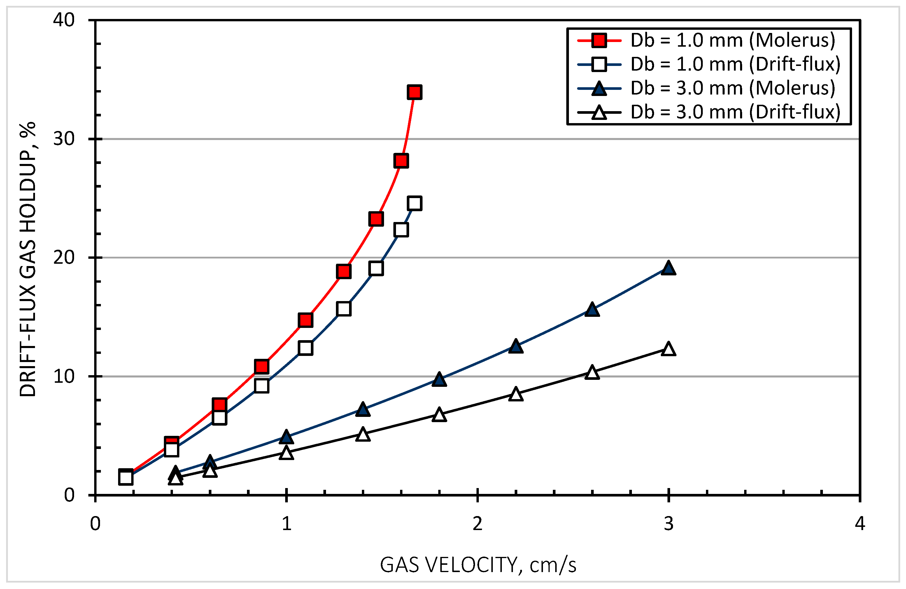
Gas holdup predictions for both models were calculated for bubble sizes up to 3 mm and superficial gas velocities up to 3 cm/s, which cover ranges of interest in flotation. The calculations were made for a 3 m diameter cell, operated in batch mode (no liquid flowrate) and at standard conditions (100,000 Pa and 20 °C). Values used in the calculations were a gravity acceleration of 980.6 cm/s² and water and air properties at 20 °C (ρ_water = 0.9983 g/cm³, µ_water = 0.01000 g/cm s, and ρ_air = 0.001205 g/cm³). The selected conditions and results of these calculations are summarized in

Table 1. Gas holdup model predictions for bubble sizes and gas velocities of interest in flotation.

Db (cm)	Drift-Flux			Molerus
	Jg (cm/s)	Sb (1/s)	εg (%)	Jg (cm/s)	Sb (1/s)	εg (%)
0.05	0.09	10.8	1.69	0.08	10.8	1.59
0.05	0.20	24.0	3.96	0.26	24.0	5.78
0.05	0.35	42.0	7.54	0.40	42.0	9.71
0.05	0.49	58.8	11.67	0.52	58.8	13.78
0.05	0.59	70.8	15.48	0.61	70.8	17.62
0.05	0.67	80.4	19.64	0.68	80.4	21.64
0.05	0.72	86.4	23.55	0.72	86.4	25.10
0.05	0.75	90.0	27.87	0.74	90.0	28.32
0.10	0.16	9.6	1.46	0.16	9.6	1.60
0.10	0.50	30.0	4.87	0.40	30.0	4.34
0.10	0.75	45.0	7.70	0.65	45.0	7.58
0.10	1.00	60.0	10.95	0.87	60.0	10.82
0.10	1.25	75.0	14.81	1.10	75.0	14.74
0.10	1.45	87.0	18.64	1.30	87.0	18.83
0.10	1.60	96.0	22.36	1.47	96.0	23.26
0.10	1.72	103.2	26.49	1.60	103.2	28.16
0.10	1.80	108.0	31.15	1.67	108.0	33.93
0.15	0.30	12.0	1.91	0.30	12.0	2.22
0.15	0.70	28.0	4.65	0.75	28.0	6.13
0.15	1.20	48.0	8.50	1.20	48.0	10.75
0.15	1.65	66.0	12.55	1.60	66.0	15.68
0.15	2.10	84.0	17.50	1.90	84.0	20.20
0.15	2.45	98.0	22.54	2.15	98.0	25.01
0.15	2.70	108.0	27.64	2.34	108.0	30.29
0.15	2.82	112.8	31.37	2.44	112.8	36.27
0.20	0.32	9.6	1.57	0.32	9.6	1.90
0.20	0.65	19.5	3.28	0.65	19.5	4.12
0.20	1.10	33.0	5.76	1.10	33.0	7.51
0.20	1.50	45.0	8.14	1.50	45.0	10.94
0.20	1.90	57.0	10.75	1.90	57.0	14.86
0.20	2.25	67.5	13.26	2.25	67.5	18.87
0.20	2.60	78.0	16.06	2.65	78.0	24.61
0.20	3.00	90.0	19.78	3.00	90.0	32.45
0.30	0.42	8.4	1.47	0.42	8.4	1.90
0.30	0.60	12.0	2.12	0.60	12.0	2.79
0.30	1.00	20.0	3.60	1.00	20.0	4.92
0.30	1.40	28.0	5.16	1.40	28.0	7.24
0.30	1.80	36.0	6.80	1.80	36.0	9.78
0.30	2.20	44.0	8.53	2.20	44.0	12.56
0.30	2.60	52.0	10.37	2.60	52.0	15.66
0.30	3.00	60.0	12.34	3.00	60.0	19.17

, which also includes corresponding values of bubble surface area flux.

Gas holdup variations as a function of gas velocity for different bubble sizes are illustrated in Figure 1 and Figure 2 for the drift-flux and Molerus models, respectively. Gas velocity values were selected to obtain approximately evenly distributed gas holdups along the range. Both models showed in every case similar trends with higher Molerus than drift-flux gas holdups for the same gas velocity and bubble size. A direct comparison of model gas holdups (Figure 3) demonstrated that the difference between Molerus and drift-flux values increased with bubble size and with gas holdup. A comparison of gas holdup values obtained at the same gas velocity for several bubble sizes (Figure 4) showed that the difference between Molerus and drift-flux predictions also increased with gas velocity.

The relationship between bubble surface area flux and gas holdup is of interest, as if proven, interfacial areas can be calculated without the need for bubble size measurements. There is evidence in the literature that a linear relationship with slope around 5.5 can be found when values of bubble surface area flux are plotted vs. gas holdup [34]. Plots of the bubble surface area flux vs. gas holdup predicted by the two models showed significant differences (Figure 5 and Figure 6). In the case of the drift-flux model, the curves for the different bubble sizes were close and approximately linear for gas holdups below 10%; a linear relationship with slope 5.5 fits this range reasonably well. However, the curves obtained with Molerus model showed a noticeable effect of bubble size.

5. Models Application

Data for the characterization of frother roles in flotation were collected in laboratory flotation cells and columns operated with frother solutions of increasing concentration. The exercise, which involves bubble size measurements and the determination of water flowrates carried by the bubbles into the froth zone, produces a data set with values of the three gas dispersion variables (superficial gas velocity, bubble size, and gas holdup) simultaneously measured in the collection zone and corrected to the same conditions of pressure and temperature. In the case of a laboratory column, this data set is hydrodynamically coherent, as the full bubble population flows through the test section where bubbles are sampled while rising at a velocity limited by the maximum level of interactions possible and developing a gas holdup measured along the full test section; this is an ideal set of gas dispersion variables to assess model predictions by comparison to calculated values.

A data set collected in one of these exercises was used to test the reliability and accuracy of the drift-flux and Molerus model predictions. Full documentation of the equipment and testing procedure is necessary to ensure that the required information to calculate values of the gas dispersion variables, at a reference set of conditions, is available. The data were collected around the top of a laboratory flotation column assembled with flanged sections of acrylic tube (Figure 7). The unit, 0.1 m in diameter and 2.2 m high, was instrumented for on-line monitoring of the differential pressure (DP) along a test section to calculate gas holdup, the solution temperature (T) to calculate gas flowrate, and the hydrostatic pressure at its bottom (P1) to calculate the pressure at its middle point; the conditions at this middle point were selected as reference to report measurements. A mass flowmeter was used to continuously control and monitor the delivery of a gas flowrate, reported at standard conditions (100,000 Pa and 20 °C), which was dispersed by injection through a stainless-steel porous cylinder. The bubble size distribution was measured using a device for bubble collection and imaging (McGill bubble size analyser) installed at the top of the column; bubbles were collected by means of a vertical sampling tube immersed from the top. Four distances are necessary for the calculation of the dispersion variables at the reference conditions: H₀, the height of the test section; H₁, the vertical distance between the top of the test section and the column overflow; H₂, the vertical distance between the column overflow and the bottom end of the bubble collection tube immersed in the column; and H₃, the vertical distance between the column overflow to the point at the centre of the area imaged to collect bubble images.

The test program, which was run on six commercial frothers provided by Flottec (F140, F150, F160-05, F160-10, F160-13, and F173), included measurements in solutions at seven concentrations (2, 5, 10, 15, 30, 60, and 100 ppm), using the same gas flowrate of 3 sL/min and keeping a 5 cm froth depth. A video-camera/monitor combination was used to track the location of the interface. The froth depth was maintained by manual adjustments of the flow of a frother solution fed to compensate for the water overflowing the column; introduction of the feed above the test section causes the rise of the bubble swarm through the test section with no counter-current liquid flowrate. Batches of 80 L of the test solution (frother in water) were prepared at room temperature (around 20 °C) for every measurement. The water overflow rate was collected into a vertical acrylic tube, 0.05 m in diameter, and measured by tracking the increasing hydrostatic pressure of the solution column formed by accumulation of the liquid (P2).

Every measurement was initiated circulating for 10 min, with the gas flowrate established: first tap water to wash the column and then the frother solution to fill the column. The selected froth depth was maintained by manual control of the level control pump. Once stable traces of the monitored variables were confirmed, data were collected for 5 min at a sampling rate of one reading every two seconds, followed by the collection of two hundred bubble images. Average values of the variables during sampling periods were used to calculate superficial gas velocity and gas holdup, while the size distribution of the bubble population was determined from automated processing of the bubble images.

The set of data is summarized in Table 2; it includes frother, solution concentration and temperature, and measured gas velocity J_g, gas holdup ε_g, and Sauter mean bubble size d_b (d₃₂). Model predictions for bubble size (calculated from measured gas velocity and gas holdup) and for gas holdup (calculated from measured gas velocity and bubble size) are also included for both models. Temperature adjustments of water and air properties were necessary in these calculations. Data were collected from two internet sites for a temperature range expected in laboratory testing and industrial units (0–40 °C):

(1)

(http://www.viscopedia.com/viscosity-tables/substances/water) accessed on 26 October 2022;

(2)

(Properties of Air at atmospheric pressure–The Engineering Mindset).

Table 2. Measured and model predicted values of gas dispersion variables obtained in the characterization of frother effects on flotation.

Frother	Conc. (ppm)	Temp. (°C)	Measurements			Model Predictions (Drift-Flux)		Model Predictions (Molerus)
			Jg (cm/s)	Db (mm)	εg (%)	Db (mm)	εg (%)	Db (mm)	εg (%)
F140	2	19.0	0.605	2.063	4.17	1.437	2.97	1.787	3.72
	5	17.5	0.601	1.581	4.96	1.214	3.82	1.451	4.61
	10	18.7	0.604	1.045	6.82	0.903	5.79	1.028	6.71
	15	17.1	0.602	0.884	8.71	0.749	7.08	0.824	8.05
	30	17.2	0.601	0.721	10.46	0.655	9.13	0.707	10.21
	60	17.6	0.604	0.607	13.21	0.567	11.77	0.599	12.94
	100	17.0	0.604	0.584	13.84	0.556	12.67	0.584	13.85
F150	2	19.9	0.606	1.993	3.82	1.567	3.06	1.993	3.82
	5	17.5	0.601	1.527	4.44	1.355	3.95	1.654	4.75
	10	17.5	0.602	1.055	6.05	1.011	5.77	1.168	6.68
	15	16.9	0.601	0.894	7.42	0.850	6.99	0.954	7.96
	30	18.6	0.606	0.621	11.90	0.599	11.24	0.639	12.40
	60	19.6	0.610	0.547	14.26	0.538	13.81	0.565	15.03
	100	20.8	0.612	0.527	15.13	0.517	14.58	0.541	15.83
F160-05	2	21.3	0.609	2.012	3.69	1.618	3.02	2.086	3.79
	5	19.0	0.604	1.821	3.85	1.558	3.33	1.972	4.10
	10	20.9	0.609	1.212	5.29	1.128	4.91	1.345	5.81
	15	19.7	0.607	0.922	7.18	0.862	6.64	0.976	7.62
	30	21.0	0.611	0.703	10.66	0.634	9.22	0.686	10.34
	60	18.1	0.606	0.607	13.25	0.565	11.74	0.597	12.91
	100	20.2	0.611	0.579	14.91	0.523	12.42	0.548	13.64
F160-10	2	9.6	0.585	2.231	3.75	1.667	2.85	2.051	3.51
	5	7.9	0.581	1.637	4.49	1.404	3.85	1.659	4.54
	10	19.1	0.605	1.101	6.23	0.976	5.47	1.128	6.37
	15	16.5	0.600	0.807	10.40	0.661	7.93	0.714	8.95
	30	18.6	0.607	0.620	12.28	0.588	11.29	0.626	12.46
	60	17.9	0.606	0.582	13.86	0.552	12.63	0.581	13.82
	100	15.9	0.602	0.566	14.69	0.543	13.60	0.568	14.77
F160-13	2	17.4	0.600	2.079	3.72	1.622	2.96	2.057	3.69
	5	17.8	0.601	1.637	4.24	1.415	3.68	1.746	4.47
	10	17.1	0.600	1.054	6.05	1.010	5.77	1.166	6.68
	15	16.7	0.600	0.841	7.87	0.811	7.52	0.903	8.51
	30	16.8	0.602	0.655	12.08	0.600	10.54	0.639	11.66
	60	20.5	0.610	0.569	13.70	0.545	12.71	0.575	13.93
	100	19.9	0.610	0.541	14.93	0.523	14.02	0.548	15.25
F173	2	15.9	0.598	1.744	3.90	1.557	3.50	1.943	4.26
	5	18.1	0.603	1.292	4.85	1.240	4.65	1.491	5.50
	10	21.1	0.610	0.837	7.84	0.796	7.38	0.894	8.42
	15	18.2	0.604	0.741	9.16	0.716	8.75	0.785	9.82
	30	19.0	0.607	0.625	11.84	0.600	11.09	0.641	12.26
	60	18.7	0.607	0.630	12.78	0.574	11.00	0.609	12.16
	100	18.3	0.607	0.627	13.14	0.567	11.15	0.600	12.31

Table 2. Measured and model predicted values of gas dispersion variables obtained in the characterization of frother effects on flotation.

Frother	Conc. (ppm)	Temp. (°C)	Measurements			Model Predictions (Drift-Flux)		Model Predictions (Molerus)
			Jg (cm/s)	Db (mm)	εg (%)	Db (mm)	εg (%)	Db (mm)	εg (%)
F140	2	19.0	0.605	2.063	4.17	1.437	2.97	1.787	3.72
	5	17.5	0.601	1.581	4.96	1.214	3.82	1.451	4.61
	10	18.7	0.604	1.045	6.82	0.903	5.79	1.028	6.71
	15	17.1	0.602	0.884	8.71	0.749	7.08	0.824	8.05
	30	17.2	0.601	0.721	10.46	0.655	9.13	0.707	10.21
	60	17.6	0.604	0.607	13.21	0.567	11.77	0.599	12.94
	100	17.0	0.604	0.584	13.84	0.556	12.67	0.584	13.85
F150	2	19.9	0.606	1.993	3.82	1.567	3.06	1.993	3.82
	5	17.5	0.601	1.527	4.44	1.355	3.95	1.654	4.75
	10	17.5	0.602	1.055	6.05	1.011	5.77	1.168	6.68
	15	16.9	0.601	0.894	7.42	0.850	6.99	0.954	7.96
	30	18.6	0.606	0.621	11.90	0.599	11.24	0.639	12.40
	60	19.6	0.610	0.547	14.26	0.538	13.81	0.565	15.03
	100	20.8	0.612	0.527	15.13	0.517	14.58	0.541	15.83
F160-05	2	21.3	0.609	2.012	3.69	1.618	3.02	2.086	3.79
	5	19.0	0.604	1.821	3.85	1.558	3.33	1.972	4.10
	10	20.9	0.609	1.212	5.29	1.128	4.91	1.345	5.81
	15	19.7	0.607	0.922	7.18	0.862	6.64	0.976	7.62
	30	21.0	0.611	0.703	10.66	0.634	9.22	0.686	10.34
	60	18.1	0.606	0.607	13.25	0.565	11.74	0.597	12.91
	100	20.2	0.611	0.579	14.91	0.523	12.42	0.548	13.64
F160-10	2	9.6	0.585	2.231	3.75	1.667	2.85	2.051	3.51
	5	7.9	0.581	1.637	4.49	1.404	3.85	1.659	4.54
	10	19.1	0.605	1.101	6.23	0.976	5.47	1.128	6.37
	15	16.5	0.600	0.807	10.40	0.661	7.93	0.714	8.95
	30	18.6	0.607	0.620	12.28	0.588	11.29	0.626	12.46
	60	17.9	0.606	0.582	13.86	0.552	12.63	0.581	13.82
	100	15.9	0.602	0.566	14.69	0.543	13.60	0.568	14.77
F160-13	2	17.4	0.600	2.079	3.72	1.622	2.96	2.057	3.69
	5	17.8	0.601	1.637	4.24	1.415	3.68	1.746	4.47
	10	17.1	0.600	1.054	6.05	1.010	5.77	1.166	6.68
	15	16.7	0.600	0.841	7.87	0.811	7.52	0.903	8.51
	30	16.8	0.602	0.655	12.08	0.600	10.54	0.639	11.66
	60	20.5	0.610	0.569	13.70	0.545	12.71	0.575	13.93
	100	19.9	0.610	0.541	14.93	0.523	14.02	0.548	15.25
F173	2	15.9	0.598	1.744	3.90	1.557	3.50	1.943	4.26
	5	18.1	0.603	1.292	4.85	1.240	4.65	1.491	5.50
	10	21.1	0.610	0.837	7.84	0.796	7.38	0.894	8.42
	15	18.2	0.604	0.741	9.16	0.716	8.75	0.785	9.82
	30	19.0	0.607	0.625	11.84	0.600	11.09	0.641	12.26
	60	18.7	0.607	0.630	12.78	0.574	11.00	0.609	12.16
	100	18.3	0.607	0.627	13.14	0.567	11.15	0.600	12.31

The data were fitted to the following polynomials using the temperature t in degrees centigrade (°C) as the variable:

$${\mathsf{\rho }}_{\mathrm{w}}={4.360\times 10}^{-8}{\mathrm{t}}^3 -{7.990\times 10}^{-6}{\mathrm{t}}^2+{5.901\times 10}^{-5}\mathrm{t}+1.000\times {10}^0$$

(18)

$${\mathsf{\mu }}_{\mathrm{w}}=-{9.211\times 10}^{-8}{\mathrm{t}}^3+{1.088\times 10}^{-5} {\mathrm{t}}^2 -{5.703\times 10}^{-4}\mathrm{t}+{1.779\times 10}^{-2}$$

(19)

$${\mathsf{\rho }}_{\mathrm{air}}={1.416\times 10}^{-8}{\mathrm{t}}^2 -{4.705\times 10}^{-6}\mathrm{t}+{1.293\times 10}^{-3}$$

(20)

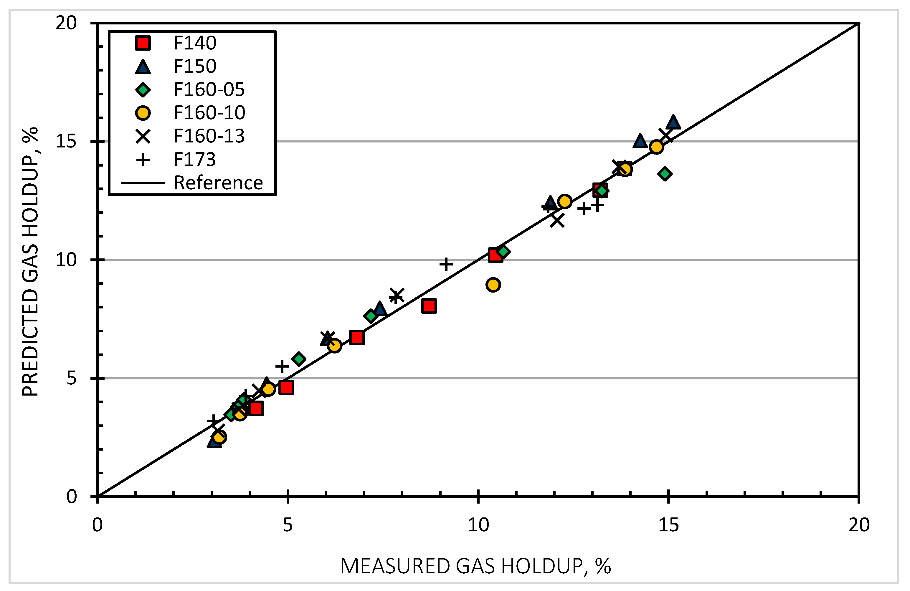
Bubble size predictions for the drift-flux and Molerus models are illustrated in Figure 8 and Figure 9, respectively. The results showed that predicted bubble sizes are systematically underestimated by the drift-flux model. Relative errors (respect to the measured bubble size) are between 10 and 30%, increasing with bubble size. Bubble size predictions using the Molerus model were lower and higher around the measured size, with values that are much closer. Relative errors are up to about 15%, with most values below 10%, and showed no effect of bubble size. In the case of the gas holdup (Figure 10 and Figure 11), predictions follow similar patterns as those exhibited by bubble size. The drift-flux model consistently underestimates gas holdup with relative errors between 10 and 30%, while results for the Molerus model showed values around the measured gas holdups with relative errors below 15% (mostly below 10%).

The results indicate that bubble size and gas holdup predictions obtained from Molerus model are closer to the measured values than those obtained from the drift-flux model. Molerus model predictions showed in most cases relative errors below 10%, which are acceptable for calculating bubble sizes in the control of cell operation. It is important to keep in mind that the test program for the data set used in the models’ assessment was not designed for this specific purpose; one limitation was that all tests were run at a single gas flowrate. The Molerus model seems to be a promising alternative for bubble size prediction, but further testing is required to assess its performance with data collected in lab and industrial mechanical cells and columns, where conditions in the test section may not be stable or homogeneous; efforts need to be made to ensure collection of a hydrodynamically coherent data set.

6. Concluding Statements

Knowledge of the characteristics of the bubble population in the collection zone of flotation equipment makes possible the effective control of individual cells and circuit performance. Three variables describe bubble populations generated by gas dispersion: superficial gas velocity, has holdup, and bubble size. A literature review revealed that current instrumentation cannot provide reliable on-line measurement of these variables except for gas velocity and that some promising alternatives for gas holdup measurement may be available in the near future; bubble size measurements will continue to be absent. The close relationships between the gas dispersion variables makes possible the development of models that allow calculation of one of the variables knowing values of the other two, which, in flotation, will provide values for the three gas dispersion variables measuring just gas velocity and holdup.

Modelling bubble flow in flotation was pursued using two approaches: determining the bubble velocity reduction by the presence of other bubbles and regarding the bubble swarm as a packed bed through which a fluid is allowed to flow. Models developed using these two approaches were searched in the literature (drift-flux and Molerus, respectively) and used to assess their prediction ability.

Gas holdup predictions for both models were calculated for bubble sizes and superficial gas velocities below 3 mm and 3 cm/s, respectively. The results showed similar trends for both models with higher gas holdup values for Molerus than drift-flux; the difference between Molerus and drift-flux values increased with bubble size and gas velocity. A relationship between bubble surface area flux and gas holdup was explored by plotting values of bubble surface area flux vs. predicted gas holdups. The results for both models showed in general an effect of bubble size that was more noticeable for the Molerus model.

A data set collected to characterize frother roles in flotation was utilized to assess model predictions for bubble size (calculated from measured gas velocity and gas holdup) and for gas holdup (calculated from measured gas velocity and bubble size). The set included values of the three gas dispersion variables measured simultaneously and reported at the same conditions. The program involved measurements in solutions of six commercial frothers for a wide range of concentrations (2 to 100 ppm). Bubble size and gas holdup predictions using the drift-flux model systematically underestimated the measured values, with relative errors between 10 and 30%. Predictions using the Molerus model showed lower and higher values around the measured value, with relative errors below 15%.

The results indicated that bubble size and gas holdup predictions obtained from the Molerus model were closer to the measured values than those obtained from the drift-flux model. Molerus model predictions showed in most cases relative errors below 10%, which are acceptable for calculating bubble sizes in the control of cell operation. It is important to keep in mind that the test program for the data set used in the models’ assessment was not designed for this specific purpose; one limitation was that all tests were run at a single gas flowrate. The Molerus model seems to be a promising alternative for bubble size prediction, but further testing is required to assess its performance with data collected in lab and industrial mechanical cells and columns, when conditions in the test section may not be stable or homogeneous. An effort needs to be made to collect hydrodynamically coherent data sets.

Both models may be improved by including data and equations developed for the behaviour of rising bubbles instead of sedimenting particles. Bubble velocity is a function of its shape, which changes in the presence of frothers and with the liquid medium viscosity, which is not the case for particles.

References

- Okasaki, S. The Velocity of Ascending Air Bubbles in Aqueous Solutions of a Surface Active Substance and the Life of the Bubble on the Same Solution. Bull. Chem. Soc. Jpn. 1964, 37, 144–150. [Google Scholar] [CrossRef]
- Gomez, C.O.; Finch, J.A. Gas Dispersion Measurements in Flotation Machines. CIM Bull. 2002, 95, 73–78. [Google Scholar]
- Gomez, C.O.; Finch, J.A. Gas Dispersion Measurements in Flotation Cells. Int. J. Miner. Process. 2007, 84, 51–58. [Google Scholar] [CrossRef]
- Gorain, B.K.; Franzidis, J.-P.; Manlapig, E.V. Studies on Impeller Type, Impeller Speed and Air Flow Rate in an Industrial Scale Flotation Cell—Part 1: Effect on Bubble Size Distribution. Miner. Eng. 1995, 8, 615–635. [Google Scholar] [CrossRef]
- Gorain, B.K.; Franzidis, J.-P.; Manlapig, E.V. Studies on Impeller Type, Impeller Speed and Air Flow Rate in an Industrial Scale Flotation Cell—Part 2: Effect on Gas Holdup. Miner. Eng. 1995, 8, 1557–1570. [Google Scholar] [CrossRef]
- Gorain, B.K.; Franzidis, J.-P.; Manlapig, E.V. Studies on Impeller Type, Impeller Speed and Air Flow Rate in an Industrial Scale Flotation Cell—Part 3: Effect on Superficial Gas Velocity. Miner. Eng. 1996, 9, 639–654. [Google Scholar] [CrossRef]
- Grau, R.A.; Heiskanen, K. Visual Technique for Measuring Bubble Size in Flotation Machines. Miner. Eng. 2002, 15, 507–513. [Google Scholar] [CrossRef]
- Grau, R.A.; Heiskanen, K. Gas Dispersion Measurements in a Flotation Cell. Miner. Eng. 2003, 16, 1081–1089. [Google Scholar] [CrossRef]
- Randall, E.W.; Goodall, C.M.; Fairlamb, P.M.; Dold, P.L.; O’Connor, C.T. A Method for Measuring the Sizes of Bubbles in Two and Three Phase Systems. J. Phys. E Sci. Instrum. 1989, 22, 827–833. [Google Scholar] [CrossRef]
- Schwarz, S.; Alexander, D. Gas Dispersion Measurements in Industrial Flotation Cells. Miner. Eng. 2006, 19, 554–560. [Google Scholar] [CrossRef]
- Gomez, C.O.; Hernandez-Aguilar, J.R.; McSorley, G.; Voigt, P.; Finch, J.A. Plant Experiences in the Measurement and Interpretation of Bubble Size Distribution in Flotation Machines. In Proceedings of the Copper 2003—The 5th International Conference, Santiago, Chile, 30 November–3 December 2003; Gomez, C.O., Barahona, C.A., Eds.; Volume III, pp. 226–240. [Google Scholar]
- Yianatos, J.; Bergh, L.; Condori, P.; Aguilera, J. Hydrodynamic and Metallurgical Characterization of Industrial Flotation Banks for Control Purposes. Miner. Eng. 2001, 14, 1033–1046. [Google Scholar] [CrossRef]
- Amelunxen, P.A.; Rothman, P. The Online Determination of Bubble Surface Area Flux Using the CiDRA GH-100 Sonar Gas Holdup Meter. IFAC Proc. Vol. 2009, 42, 156–160. [Google Scholar] [CrossRef] [Green Version]
- Gomez, C.O.; Cortes-Lopez, F.; Finch, J.A. Industrial Testing of a Gas Holdup Sensor for Flotation Systems. Miner. Eng. 2003, 16, 493–501. [Google Scholar] [CrossRef]
- Maldonado, M.; Gomez, C.O. A new Approach to Measure Gas Holdup in Industrial Flotation Machines—Part I: Demonstration of Working Principle. Miner. Eng. 2018, 118, 1–8. [Google Scholar] [CrossRef]
- O’Keefe, C.; Viega, J.; Fernald, M. Application of Sonar Technology to Mineral Processing and Oil Sands Applications. In Proceedings of the 39th Annual Canadian Mineral Processors Conference 2007; Paper 26; CIM: Ottawa, ON, Canada, 2007; pp. 429–457. [Google Scholar]
- Banisi, S.; Finch, J.A. Technical Note: Reconciliation of Bubble Size Estimation Methods Using Drift Flux Analysis. Miner. Eng. 1994, 7, 1555–1559. [Google Scholar] [CrossRef]
- Dobby, G.S.; Yianatos, J.B.; Finch, J.A. Estimation of Bubble Diameter in Flotation Columns from Drift Flux Analysis. Can. Met. Quart. 1988, 27, 85–90. [Google Scholar] [CrossRef]
- Filippov, L.O.; Javor, Z.; Piriou, P.; Filippova, I.V. Salt Effect on Gas Dispersion in Flotation Column—Bubble Size as a Function of Turbulent Intensity. Miner. Eng. 2018, 127, 6–14. [Google Scholar] [CrossRef]
- Yianatos, J.; Finch, J.A.; Dobby, G.S.; Xu, M. Bubble Size Estimation in a Bubble Swarm. J. Colloid Interface Sci. 1988, 126, 37–44. [Google Scholar] [CrossRef]
- Alexander, K.S.; Dollimore, D.; Tata, S.S.; Uppala, V. A Comparison of the Coefficients in the Richardson and Zaki’s and Steinour’s Equations Relating to the Behaviour of Concentrated Suspensions. Sep. Sci. Technol. 1991, 26, 819–829. [Google Scholar] [CrossRef]
- Richardson, R.F.; Zaki, W.N. Sedimentation and Fluidisation: Part I. Trans. Inst. Chem. Eng. 1954, 32, 35–53. [Google Scholar] [CrossRef]
- Zuber, N. On the Dispersed Two-phase Flow in the Laminar Flow Regime. Chem. Eng. Sci. 1964, 19, 897–917. [Google Scholar] [CrossRef]
- Molerus, O. Principles of Flow in Disperse Systems; Chapman & Hall: London, UK, 1993; pp. 12, 27, 29, 70–83. [Google Scholar]
- Wallis, J.B. One Dimensional Two-Phase Flow; McGraw-Hill: New York, NY, USA, 1969; Chapter 4; pp. 89–105. [Google Scholar]
- Clift, R.; Grace, J.R.; Weber, M.E. Bubbles, Drops and Particles; Academic Press: New York, NY, USA, 1978; pp. 34–35, 111. [Google Scholar]
- Gomez, C.O.; Maldonado, M.; Araya, R.; Finch, J.A. Frother and Viscosity Effects on Bubble Shape and Velocity; Rheology in Mineral Processing; Pawlik, M., Ed.; MetSoc: Quebec, QC, Canada, 2010; pp. 57–73. [Google Scholar]
- Karamanev, D.G. Equations for Calculations of the Terminal Velocity and Drag Coefficient of Solids Spheres and Gas Bubbles. Chem. Eng. Commun. 1996, 147, 75–84. [Google Scholar] [CrossRef]
- Sam, A.; Gomez, C.O.; Finch, J.A. Axial Velocity Profiles of Single Bubbles in Water/Frother Solutions. Int. J. Miner. Process. 1996, 47, 177–196. [Google Scholar] [CrossRef]
- Zhang, Y.; McLaughlin, J.B.; Finch, J.A. Bubble Velocity Profile and Model of Surfactant Mass Transfer to Bubble Surface. Chem. Eng. Sci. 2001, 56, 6605–6616. [Google Scholar] [CrossRef]
- Chegeni, M.H.; Abdollahy, M.; Khalesi, M.R. Column Flotation Cell Design by Drift Flux and Axial Dispersion Models. Int. J. Miner. Process. 2015, 145, 83–86. [Google Scholar] [CrossRef]
- Masliyah, J.H. Hindered Settling in a Multi-Species Particle System. Chem. Eng. Sci. 1979, 34, 1166–1168. [Google Scholar] [CrossRef]
- Wilhem, R.H.; Kwauk, M. Fluidization of Solid Particles. Chem. Eng. Prog. 1948, 44, 201–218. [Google Scholar]
- Finch, J.A.; Xiao, J.; Hardie, C.; Gomez, C.O. Gas Dispersion Properties: Bubble Surface Area Flux and Gas Holdup. Miner. Eng. 2000, 13, 365–372. [Google Scholar] [CrossRef]
Figure 1.
Gas holdup predictions for selected bubble sizes and gas velocities (drift-flux model).
Figure 2.
Gas holdup predictions for selected bubble sizes and gas velocities (Molerus model).
Figure 3.
Comparison of gas holdup model predictions for selected bubble sizes and gas velocities.
Figure 4.
Gas holdup model predictions vs. gas velocity for selected bubble sizes.
Figure 5.
Bubble surface area flux vs. gas holdup prediction (drift-flux model).
Figure 6.
Bubble surface area flux vs. gas holdup prediction (Molerus model).
Figure 7.
Relevant lengths and distances in the measurements of gas dispersion variables in a laboratory flotation column.
Figure 8.
Predicted vs. measured bubble size (drift-flux model).
Figure 9.
Predicted vs. measured bubble size (Molerus model).
Figure 10.
Predicted vs. measured gas holdup (drift-flux model).
Figure 11.
Predicted vs. measured gas holdup (Molerus model).