
3D Focusing Inversion of Full Tensor Magnetic Gradiometry Data with Gramian Regularization


1
Department of Geology and Geophysics, University of Utah, Salt Lake City, UT 84112, USA
2
TechnoImaging, Salt Lake City, UT 84107, USA
3
Vale Canada Limited, Toronto, ON M5J 2K2, Canada
*
Author to whom correspondence should be addressed.
Minerals 2023, 13(7), 851; https://0-doi-org.brum.beds.ac.uk/10.3390/min13070851
Submission received: 9 May 2023
/
Revised: 17 June 2023
/
Accepted: 20 June 2023
/
Published: 23 June 2023
(This article belongs to the Special Issue Feature Papers in Mineral Exploration Methods and Applications 2022)
Abstract
:Full tensor magnetic gradiometry (FTMG) is becoming a practical method for exploration due to recent advancements in superconducting quantum interference device (SQUID) technology. This paper introduces an efficient method of 3D modeling and inversion of FTMG data. The forward modeling uses single-point Gaussian integration with pulse basis functions to compute the volume integrals representing the second spatial derivatives of the magnetic potential. The inversion is aimed at recovering both the magnetic susceptibility and magnetization vectors. We have introduced a 3D regularized focusing inversion technique that utilizes Gramian regularization and a moving sensitivity domain approach. We have also developed a new method of magnetization vector decomposition into induced and remanent parts. The case study includes applying the developed inversion method and computer code to interpret a helicopter-borne FTMG survey carried out over the Thompson Nickel Belt. We have analyzed and separately inverted the observed FTMG and total magnetic intensity (TMI) data using the developed 3D inversion methods to obtain the subsurface susceptibility and magnetization vector models. Furthermore, we present a comparison of the inversions utilizing the FTMG data and the TMI data.
1. Introduction
The measurement of magnetic vector data using orthogonal fluxgate magnetometers is heavily influenced by the Earth’s magnetic field and can be greatly affected by the orientation of the instruments. Therefore, due to the instability of airborne platforms, cesium vapor magnetometers have been preferred as they directly measure the total magnetic intensity (TMI) and are not affected by instrument orientation.
Despite this, direct measurements of magnetic tensors have advantages, as they contain directional sensitivity, which is important for determining rock magnetization vector and studying remanent magnetization. Recently, full tensor magnetic gradiometers based on superconducting quantum interference devices (SQUIDs) have been developed and are now commercially used for geophysical surveying (e.g., [1,2,3,4]). The quantum magnetic tensor (QMAGT) system, developed by Dias Airborne of Saskatoon, Saskatchewan, Canada in collaboration with Supracon AG of Jena, Thuringia, Germany, is a helicopter-borne magnetic survey system that measures the FTMG data using the SQUID, operating within a liquid helium bath (https://www.diasgeo.com/technology-innovation/full-tensor-magnetic-gradiometry-ftmg/, accessed on 21 June 2023).
Inverting the data obtained from full tensor magnetic gradiometry into a magnetization vector through 3D inversion remains a challenging problem [4,5]. In this paper, we present recent advances in FTMG data modeling and inversion and illustrate the developed methods using the results of a helicopter-borne QMAGT FTMG survey conducted over the Thompson Nickel Belt near Thompson, Manitoba, Canada.
We also demonstrate that the inversion of FTMG data has several advantages over traditional TMI data for mineral exploration. TMI data usually require significant post-processing before inversion, such as arbitrary filtering, but FTMG data are naturally high-frequency and require only minimal post-processing, such as leveling and outlier removal, before inversion. Furthermore, the FTMG data are less sensitive to instrument orientation than TMI data because magnetic gradients are mainly caused by localized sources rather than the Earth’s background field or regional trends. However, the depth sensitivity of FTMG data is limited, typically to about 600 m below the surface, whereas TMI data can penetrate several kilometers below the surface.
2. Modeling of FTMG Data for the Models without Remanent Magnetization
In what follows, we assume first that there is no remanent magnetization, the impact of self-demagnetization is insignificant, and the magnetic susceptibility is uniform in all directions. Given these assumptions, the magnetization intensity I(r) can be directly linked to the inducing magnetic field, H0(r), through the magnetic susceptibility, χ(r):
We discretize the 3D earth model into a grid of Nm cells, each of constant magnetic susceptibility. Following [10], the magnetic potential can be expressed in discrete form as follows:
where is the whole-space Green’s function for the magnetic potential:
As we will show, all components of the magnetic field can be computed as the spatial derivatives of Equation (2). For example, the magnetic field, H(r), is the first derivative of the magnetic potential:
Substituting Equation (2) into (3), we arrive at the following discrete form:
where denotes the point of observation; denotes the point of source location; and and are the direction of magnetization and the absolute value of the inducing magnetic field, H0, respectively.
In our chosen coordinate system, we consider positive y as the north direction, positive x as the east direction, and positive z as the downward direction. When conducting a magnetic survey, the inclination (I), declination (D), and azimuth (A) of the inducing magnetic field (measured in degrees) can be determined by referencing the International Geomagnetic Reference Field (IGRF) model. Under these assumptions, the components of the unit vector in the direction of the inducing magnetic field are as follows:
Previous studies (e.g., [11]) have provided analytical solutions for calculating the volume integral described in Equation (4) for right rectangular prisms with magnetic susceptibility. However, we choose to perform the volume integral computation numerically using single-point Gaussian integration with pulse basis functions, as proposed by [12]. This method dramatically speeds up the processing time compared to the conventional approach based on prismatic cell approximation while yielding a very accurate result. In this case, denotes the cell center. We assume constant discretization of ∆x, ∆y, and ∆z in the x, y, and z directions, respectively.
Thus, Equation (4) can be simplified as follows:
From Equation (8), we can derive discrete expressions for the scalar components of the magnetic field:
where
In the case of studying the full magnetic tensor, one has to calculate the second derivatives of the magnetic potential as follows:
The second spatial derivatives of the magnetic potential form a symmetric tensor with zero trace:
where
This implies that of the nine tensor components, only five are independent.
After some algebra, we find discrete forms for each component of the magnetic tensor [13]:
where t is defined by Equation (12), and
Equations (16) through (24) provide the basis for computing the FTMG data for the models without the remanent magnetization.
3. Magnetization Vector Decomposition into Induced and Remanent Parts
Conventional inversions for magnetic susceptibility only consider induced magnetization, which limits their ability to provide a comprehensive geological understanding [4,14,15]. In order to obtain an adequate understanding of geology and mineralization and recover information about remanent magnetization, magnetic data must be inverted towards a magnetization vector model. This paper presents a new method for determining remanent magnetization using the magnetization vector decomposition technique. This method decomposes the full magnetization vector into the induced (inline relative to the inducing) and remanent components (Figure 1). The amplitude of the inline magnetization can provide models similar to susceptibility since paramagnetic and ferromagnetic materials tend to align parallel to the inducing field, while diamagnetic materials tend to align in the opposite direction. The remanent magnetization can manifest itself as a vector pointing away from the inducing field (Figure 1). We illustrate this novel method for direct imaging of remanent magnetization, which is useful for determining optimal exploration strategies.
Remanent magnetization (or remanence) is a permanent magnetization of a rock obtained in the past when the Earth’s magnetic field had a different magnitude and direction than it has today. It follows that the total intensity of magnetization, I(r), is linearly related to both the induced, Mind, and remanent, Mrem, magnetizations:
where the induced magnetization vector, Mind, is linearly proportional to the inducing magnetic field, H0(r), through the magnetic susceptibility, χ(r):
and l the unit vector in the direction of the inducing magnetic field, defined by Equations (5)–(7). We should note that we have defined the magnetization vectors (both the induced, Mind, and remanent, ) as unitless for convenience of derivations.
The Koenigsberger ratio, Q, is the ratio of the absolute values of the remanent magnetization to the induced magnetization [16]:
For Koenigsberger ratios greater than 1, the remanent magnetization vector is the predominant contribution to the total intensity of magnetization [17].
We can rewrite Equation (25) as follows:
where M is the dimensionless magnetization vector:
At the same time, one can also consider a simplified alternative method to decompose the full magnetization vector into the induced and remanent components. This involves finding the magnitude of the projection of the vector onto the inducing field direction. This is termed the inline component, which is a proxy for induced magnetization. We then calculate the magnitude of vector elements that are not parallel, which we term the perpendicular component. These elements are not necessarily perpendicular, but they are not parallel to the inducing field, and this “perpendicular” term is the proxy for remanent magnetization.
4. Modeling of FTMG Data for the Models with Remanent Magnetization
For the modeling of magnetic data, we discretize the 3D earth model into a grid of Nm cells, each of a constant magnetization vector. Following [10], the magnetic field can be expressed in discrete form as follows:
where is the magnetization vector of the k-th cell.
Closed-form solutions for the volume integral in Equation (30) over right rectangular magnetic prisms have been previously presented (e.g., [11]). As discussed in [12], we prefer to evaluate the volume integral numerically using single-point Gaussian integration with pulse basis functions because this numerical solution is as accurate as the analytic solution, provided that the depth to the center of the cell exceeds twice the dimension of the cell. In this case, now denotes the center of the cell. We assume constant discretization of ∆x, ∆y, and ∆z in the x, y, and z directions, respectively. It follows that Equation (30) can be simplified as follows:
From Equation (31), we obtain discrete expressions for the vector components of the magnetic field:
where
We can write Equations (32)–(34) in a compact form as follows:
The second spatial derivatives of the magnetic potential,
form a symmetric magnetic tensor
with zero trace
where
As for the case without the remanent magnetization considered above, this implies that of the nine tensor components, only five are independent.
By introducing and after some algebra, we find discrete forms for each component of the magnetic tensor:
We now take the derivatives:
where
Substituting Equation (42) into (41), we obtain
According to (35), we can write
and
Substituting (44) and (45) into (43), we have
We introduce a sensitivity kernel for magnetic tensor as follows:
Using this notation, we can rewrite Equation (46) in the following compact form:
where are the components of the magnetization vector:
Equations (36) and (48) are the key equations that we need for solving both modeling and inversion for remanent magnetization. Note also that any implementation of these equations includes both topography and variable flight height, obviating the need for upward continuation of the data.
5. Principles of Inversion
Regardless of the iterative scheme used, most regularized inversions seek to minimize the Tikhonov parametric functional, :
where is a misfit functional of the observed and predicted potential field data, is a stabilizing functional, and is the regularization parameter that balances the misfit and stabilizing functionals [10,18]. Data and model weights can be introduced to Equation (50) through data and model weighting matrices. The purpose of these weighting matrices is to adjust the inverse problem in logarithmic space, thereby decreasing the range of variation in both the data and model parameters.
In our specific implementation, the weights assigned to the data and model are determined by considering their integrated sensitivity, as originally introduced in [19]. The concept of sensitivity weighting in geophysical inverse problems was also discussed in a number of publications, e.g., [20,21] and many others. The interested reader can find a detailed description of the theory of sensitivity weighting applied to general linear and nonlinear inverse problems in the textbooks by Zhdanov [12,18]. The sensitivity-based weighting functions ensure that the various components of the observed data exhibit equal sensitivity to cells situated at different depths and horizontal positions. Consequently, the sensitivity-based weighting functions inherently incorporate necessary adjustments for the vertical and horizontal distribution of susceptibility. This distinction represents a key difference between our approach and the geometric depth weighting functions devised by [22]. Another critical issue of the potential field inversion is the nonuniqueness of the inverse model. This question was addressed in hundreds of published papers and monographs, including those cited above. The most general approach to overcoming inherent nonuniqueness is based on the regularization theory. The nonuniqueness of the inversion is significantly reduced by bringing the a priori information via a regularization. For example, in our paper, we use Gramian and focusing regularization, which forces a level of structural similarity between the magnetization vector components.
Every geological constraint is expressed as a form of regularization, which can be measured by adjusting data weights, establishing upper and lower bounds for the model, determining model weights, incorporating prior knowledge, and selecting an appropriate stabilizing functional. The stabilizing functional incorporates information about the category of models utilized in the inversion process. The selection of a suitable stabilizing functional should rely on the user’s geological understanding. In the following section, we will provide a concise overview of various smooth and focusing stabilizers, showcasing the outcomes obtained from the 3D inversion of magnetic vector and tensor data for each approach. A minimum norm (MN) stabilizer will seek to minimize the norm of the difference between the current model and an a priori model:
and usually produces a relatively smooth model (where m = m(r) is some function describing the model parameters).
The first derivative (FD) stabilizer implicitly introduces smoothness as the first spatial derivatives of the model parameters:
and can result in spurious oscillations and artifacts when the model parameters are discontinuous. A combination of stabilizers (51) and (52) is often used (e.g., [22]).
In reality, the majority of geological formations do not possess smooth magnetization distributions. Geology often displays distinct boundaries with sharp contrasts in susceptibility, such as those observed between an ore deposit and its surrounding rock, or at a discontinuity. Consequently, the application of stabilizers (51) and (52), or their combinations, leads to results that lack physical relevance to the actual geological conditions. To address this limitation, ref. [23] introduced focusing stabilizers that enable the recovery of models with sharper boundaries and greater contrast. In this paper, we consider the minimum support (MS) stabilizer:
where e is a focusing parameter introduced to avoid singularity when .
The minimum support stabilizer aims to minimize the volume that deviates from the a priori model, thereby promoting the recovery of compact bodies. Consequently, any smooth distribution of model parameters with only minor deviations from the a priori model is penalized.
While variations of Equation (53) were derived in [10,12], we base our solution on the re-weighted regularized conjugate gradient method (RRCG) [10,18], which is easier to implement numerically.
In numerical dressing, the corresponding parametric functional can be written as follows:
where Wd is the weighting matrix for the data, and Wm is a diagonal matrix for weighting the model parameters based on integrated sensitivity, (), where is the Frechet derivative of the forward operator:
Matrix We is a diagonal matrix, determined by the discrete values of the model parameters, mi, representing the action of the minimum support stabilizer [10]:
where e is a small number (focusing parameter).
The minimization problem (50) can be reformulated using a space of weighted parameters:
where .
Equation (54) can be rewritten as follows:
where is a new forward operator in the space of weighted parameters, which can be related to the forward operator A in the original space as
The algorithm of the re-weighted regularized conjugate gradient method to solve the minimization of parametric functional (58) is given in Appendix A.
The inversion process continues through iterations until one of the following conditions is met: the residual error reaches a predetermined threshold, the decrease in error between consecutive iterations is smaller than the preset threshold, or the maximum number of iterations is reached. Once the inversion is completed, the quality of the results is assessed based on the data misfit and through visual examination of the model. As we discussed above, in practical applications of the inversion method, some boundary conditions must be imposed on the variations of the model parameters:
where and are the lower and upper limits of the model parameter . However, during the process of minimization of the Tikhonov parametric functional, we can obtain the values of the model parameters outside the above boundaries. In order to limit the interval of possible values of the inverse problem solution, one can introduce a new model parameter with the property that the corresponding original model parameter m will always remain within the imposed above boundaries and . One way to solve this problem is by using the following logarithmic transformation to arrive at new model parameters:
The corresponding inverse transformation is given by the following formula:
It is evident that conducting the inversion process in the logarithmic space of model parameters, denoted as , guarantees that the transformed value of each , regardless of its magnitude, will always remain within the predefined intervals defined by and . The details of the RRCG algorithm used to solve the inverse problem in the logarithmic space of model parameters are provided in the Appendix A.
6. Gramian Stabilizer
Inverting for the magnetization vector is a more challenging problem than inverting for scalar magnetic susceptibility, because we have three unknown scalar components of the magnetization vector for every cell. At the same time, there is inherent correlation between the different components of the magnetization vector. The different scalar components have similar spatial variations and represent the same zones of anomalous magnetization. Therefore, it is possible to expect that the different components of the magnetization vector should be mutually correlated [15,24]. It was demonstrated in [25] that one can enforce the correlation between the different model parameters by using the Gramian constraints. Following the cited paper, we have included the Gramian constraint in Equation (50) as follows:
where m is the 3Nm length vector of magnetization vector components; is the Nm length vector of the component of magnetization vector, ; is the Nm length vector of the effective magnetic susceptibility, defined as the magnitude of the magnetization vector,
Using the Gramian constraint (65), we enhance a direct correlation between the scalar components of the magnetization vector with , which is computed at the previous iteration of an inversion and is updated on every iteration. The advantage of using the Gramian constraint in the form of Equation (65) is that it does not require any a priori information about the magnetization vector (e.g., direction, the relationship between different components, etc.).
The minimization problem in Equation (63) is solved using the re-weighted regularized conjugate gradient (RRCG) method described above.
Finally, the regularized inversion outlined above can be applied to very-large-scale problems by incorporating the concept of the moving sensitivity domain [9,26]. According to this concept, the sensitivity matrix for the entire large-scale model could be constructed via the superposition of sensitivity domains for all observation points. The sensitivities are also computed “on the flight” during the computations without storing them in the computer memory. This approach makes it possible to invert the data collected by surveys of several thousand line km on a modest PC cluster as one inversion run.
For example, in our case study presented below, we employ a 10 km size of the sensitivity domain, which results in the sensitivity matrix taking up less than 100 GB of memory even on a fine grid discretization (25 m × 25 m laterally with a reasonable number of vertical layers—less than 50). Calculation of the sensitivity for this sensitivity domain takes only a few minutes. Calculation of the sensitivity matrix for an entire area—say 100 km to a side with the same discretization—can take hours or days on a single CPU or GPU with ~200 GB memory.
7. Determining the Remanent Magnetization
The separation of the magnetization vector into the parts responsible for remanent and induced polarization is a challenging problem if no a priori information is available. However, this problem can be solved approximately, assuming that the susceptibility only inversion produced the correct magnetic susceptibility distribution in the rock formations.
Taking into account Equations (25) and (28), we can find the vector of remanent magnetization Mrem as follows:
where according to Equation (26),
where l is the unit vector in the direction of the inducing magnetic field defined by Equations (5)–(7).
The unknown susceptibility, , can be found by susceptibility only inversion of the observed data. On the next step, we invert the data for the magnetization vector, . Finally, we can find the remanent magnetization by substituting Equation (67) into (66):
We should emphasize that the value of remanent magnetization determined by Formula (68) is correct if we use the true values of magnetic susceptibility . In the case when is found by susceptibility only inversion, Formula (68) can be used as some approximation for the remanent magnetization.
Based on Equation (68), one can determine the Koenigsberger ratio, Q:
If we assume that the earth model has the susceptibility of free space, , the vector of induced magnetization is constant,
Therefore, we arrive at the following equation for the remanent magnetization:
We can approximately calculate the Koenigsberger ratio, Q, as follows:
8. Model Study: Inversion of the TMI and FTMG Data for Synthetic Model
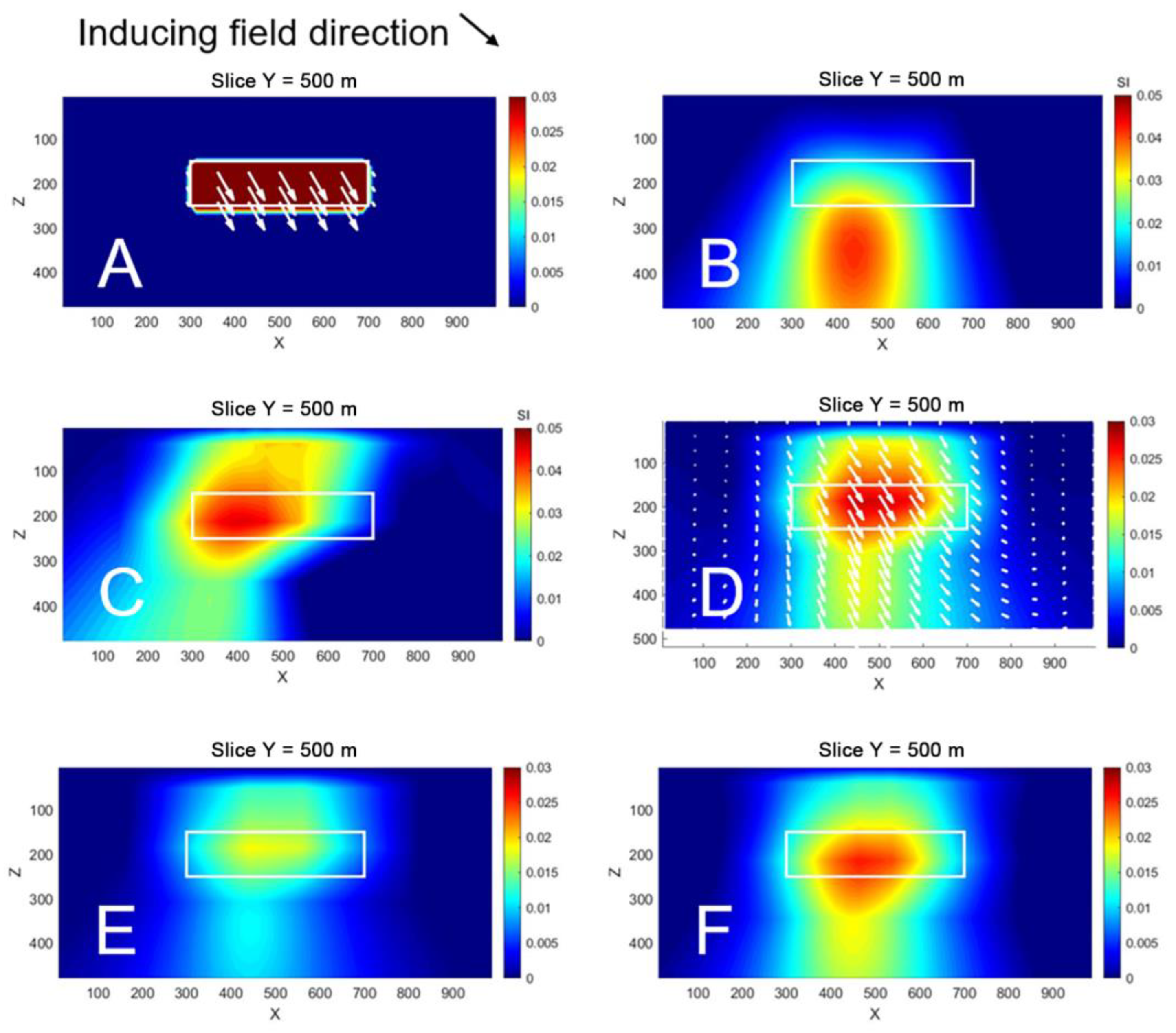
We first conducted a synthetic model study using the developed method and computer code. Figure 2 represents the vertical sections of the magnetized target and the inversion results. The anomaly in red in panel (A) has a susceptibility of 0.1 SI and amplitude of dimensionless magnetization vector 0.1 in a homogeneous background of zero elsewhere. Magnetization vector anomaly has a magnitude of 0.1 in the direction shown by the white arrows. The inclination is 75 degrees, and the declination is 35 degrees. The inducing magnetic field (indicated by the black arrow at the top of Figure 2) has an inclination of 45 degrees and a declination of 5 degrees. This is 30 degrees offset from the direction of the magnetization vector in both inclination and declination, which indicates the presence of “remanent” magnetization in this model. We have calculated the synthetic observed TMI and FTMG data using the vector magnetization model described above.
We ran inversions of the synthetic data for the magnetic susceptibility model first. Panel (B) shows the susceptibility model obtained from the inversion of the synthetic TMI data. Panel (C) shows the susceptibility model obtained from the inversion of synthetic FTMG data. One can see that TMI data inversion has difficulties recovering the correct susceptibility model; the image is diffused and slightly shifted down. At the same time, the FTMG inversion solves this problem more accurately (Panel (C)).
In the next step of this numerical experiment, we run inversion for the magnetization vector model. Panel (D) shows the magnetization vector model obtained from the inversion of synthetic FTMG data. The white arrows show the full magnetization vector, while the color map represents the amplitude of this vector. We can see the reasonable correlation between the inverse magnetization vector and the actual magnetization vector model shown in Panel (A).
Finally, Panels (E) and (F) show the color maps of the inline and “remanent” magnetization amplitudes, respectively. The stronger values in Panel (F) indicate that the anomalous body possesses “remanent” magnetization, responsible for a deviation of the magnetization vector from the inducing magnetic field indicated by the black arrow at the top of Figure 2.
9. Case Study: Inversion of the TMI and FTMG Data in the Thompson Nickel Belt in Northern Manitoba, Canada
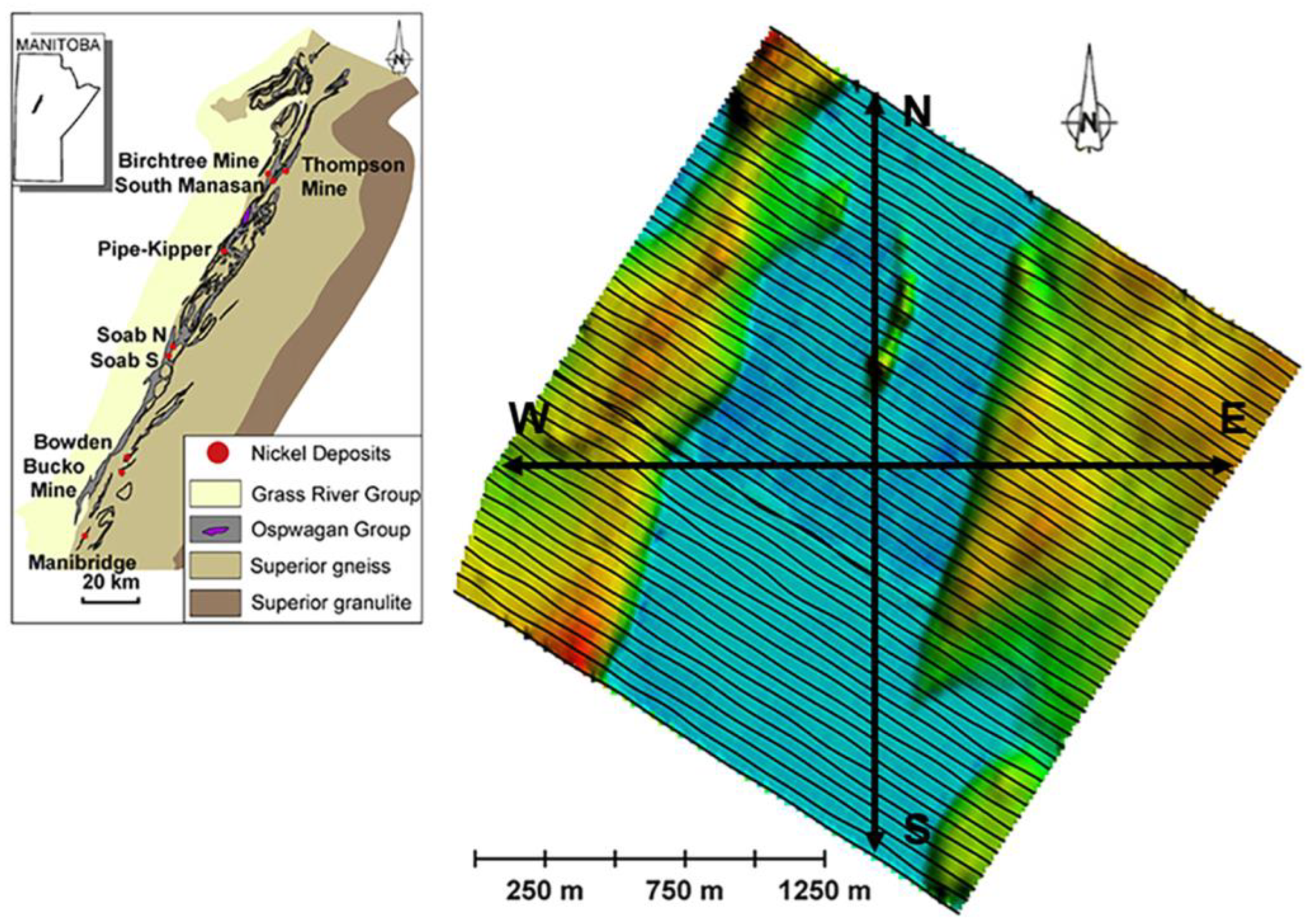
Dias Airborne collected approximately 10,655 line-km of QMAGT FTMG data in the Thompson Nickel Belt in northern Manitoba, Canada. The survey aimed to determine the gross geomorphology of the Thompson Nickel Belt which is part of the fifth-largest nickel camp in the world and the associated Ni sulfide mineralization [27,28]. This paper focuses on a small area of interest (AOI) in the northern extent of Thompson Nickel Belt near Mystery Lake, covered by approximately 100 line km. The line spacing was 50 m, with sampling every ~2.5 m, and the flight height was around 40 m. The digital terrain model (DTM) and flight lines over the AOI are shown in Figure 3.
9.1. Susceptibility and Magnetization Vector Models Produced by Inversion of FTMG Data
We conducted separate inversions of the FTMG data to obtain models for both susceptibility and magnetization vector. The inversions used a 20 m × 40 m grid with 48 vertical layers ranging from 10–95 m, but the models were ultimately limited to a depth of 600 m based on the sensitivity study. The Tikhonov regularization method with minimum support stabilizer was employed to produce focused images of magnetized structures [10,18,23,29]. The focusing regularization in Equation (53) was used in the inversions with a focusing epsilon of 0.001 which was not varied during the inversion.
Figure 4 displays observed and predicted data for selected FTMG components from the magnetization vector inversion, with the total L2 norm misfit between observed and predicted data for all six magnetic tensor components being less than 10%.
In this study, the inversion parameters for the magnetization vector model were the X, Y, and Z components of the triaxial vector. The inverse models were represented by three characteristics of the full magnetization vector, namely amplitude, inline amplitude (representing induced magnetization), and approximate amplitude of the remanent magnetization. Additionally, the projection of the full magnetization vector was shown as black arrows over the amplitude in the vertical section.
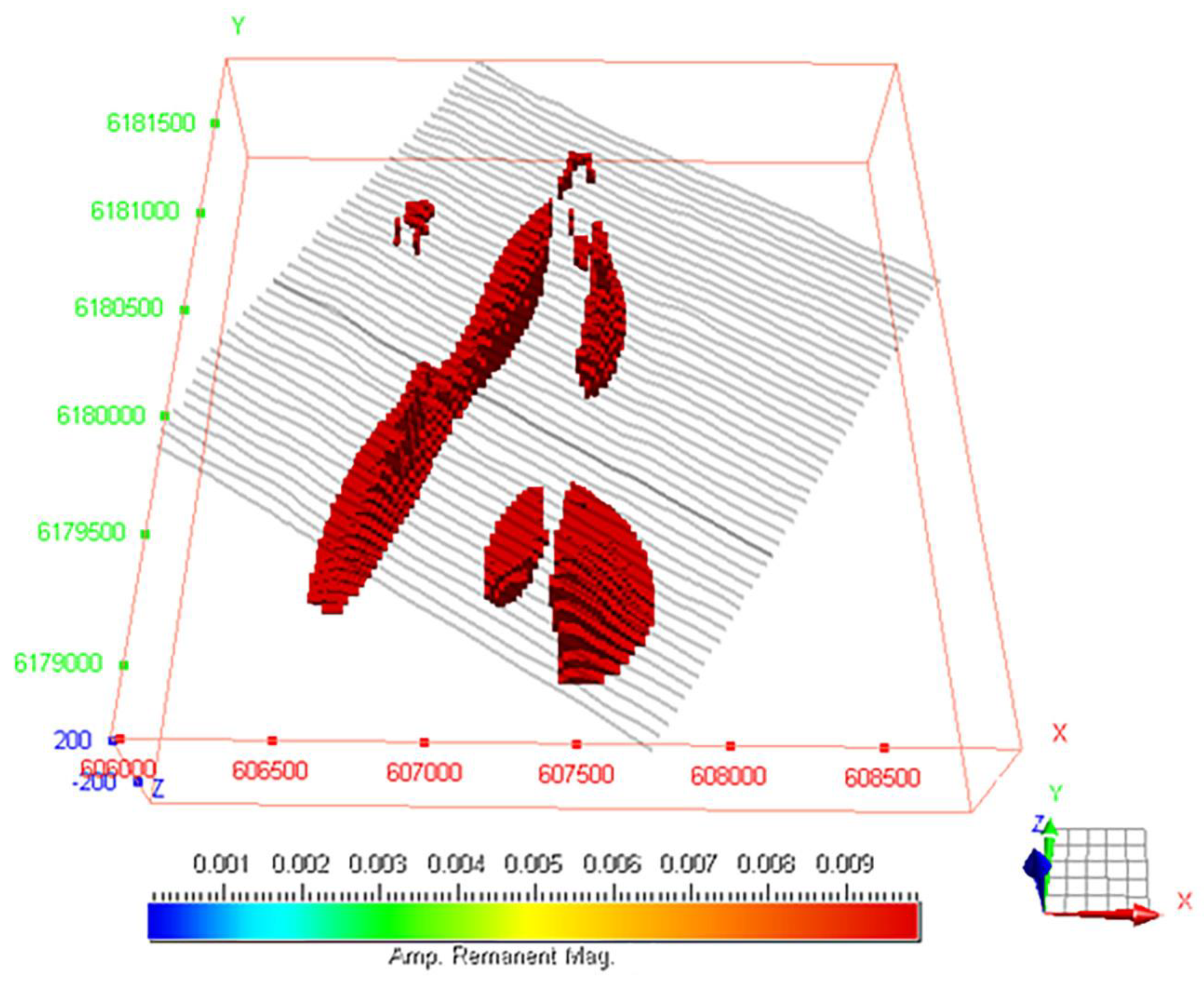
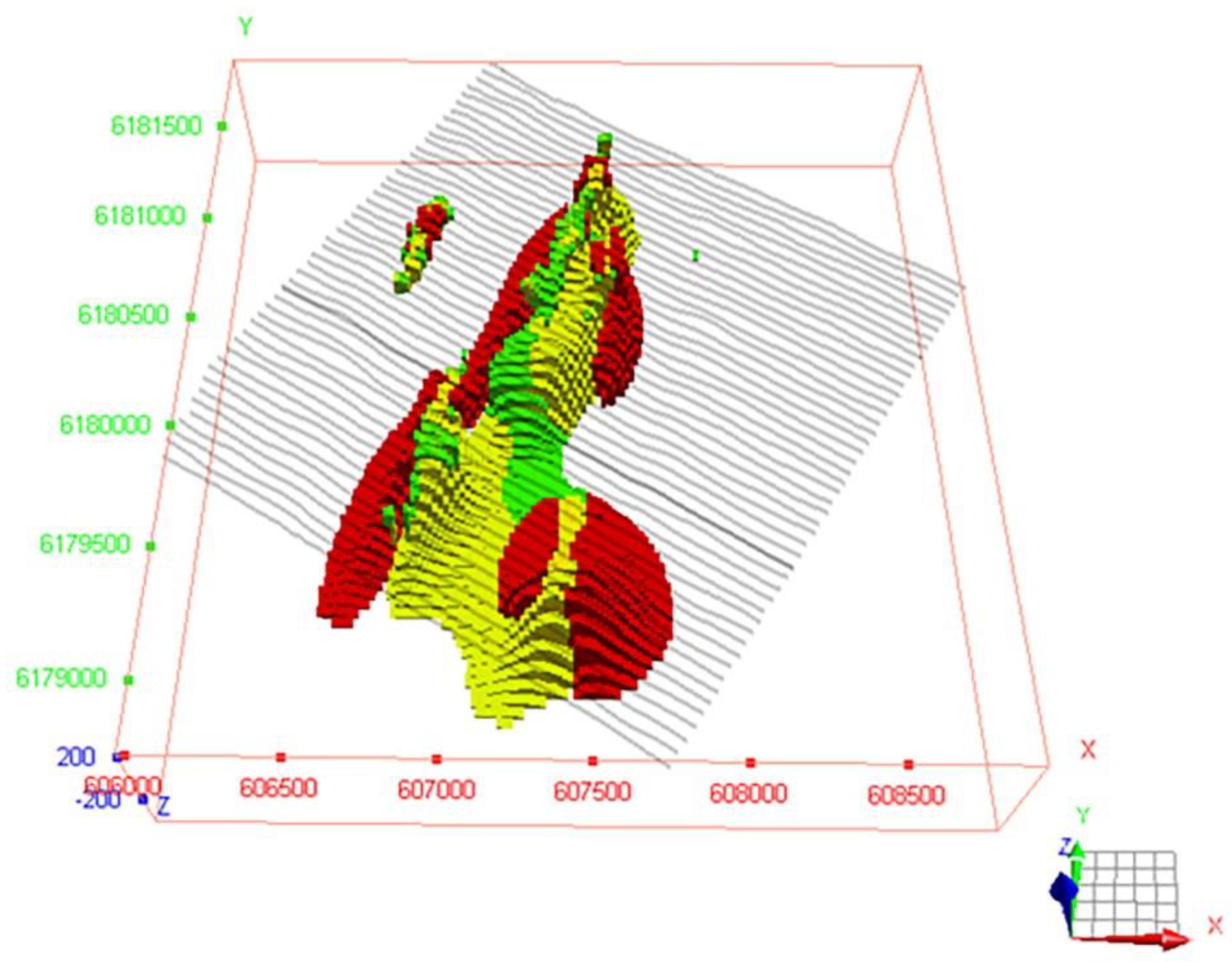
Figure 5, Figure 6, Figure 7 and Figure 8 give a 3D overview of the inverted models. Figure 5 is a 3D isobody view of the inverted susceptibility model with values greater than 0.1 SI shown in green. This isobody is the mystery ultramafic intrusion. The ultramafic body itself is not an economic resource although it does contain some nickel. Figure 6 is a 3D isobody view of the inverted inline magnetization model, which is a proxy for induced magnetization. Values above 0.02 A/m are shown in yellow and represent the same ultramafic intrusion. We see the enhanced resolution of the body versus the susceptibility model shown in Figure 5. Koenigsberger ratios () corresponding to the ultramafic ranged from 1 to 2, indicating a degree of remanence, which is consistent with the difference we see in the susceptibility and inline magnetization models. Figure 7 is a 3D isobody view of the remanent magnetization model, with values over 0.04 A/m shown in red. These red isobodies are potentially breccia-associated mineralization within the Mystery Lake ultramafic coupled with minor sedimentary sulfides which occurs within the package of Pipe Formation rocks. values were much higher in the breccia-associated mineralized zone, ranging from 5 to 5.5. These values were a factor in our choice of cutoff values for the isobodies shown. We may also see some circulation of the field in this component due to the approximate decomposition to inline and perpendicular magnetization. This is a powerful result of the MVI versus the susceptibility inversion in that we can image the target mineralization directly with the various products of the MVI. Finally, Figure 8 shows a composite view of the isobodies presented in Figure 5, Figure 6 and Figure 7.
Figure 9 depicts the S–N profiles of the inverted susceptibility and magnetization vector models. The ultramafic intrusion is clearly visible in the susceptibility and inline magnetization models as high values indicated by warm colors. However, in the remanent magnetization model, the intrusion appears as low values, indicated by cool colors, while the country rocks are shown as high values. This technique allows for better identification of potential mineralization targets by imaging the lithologies near the intrusion.
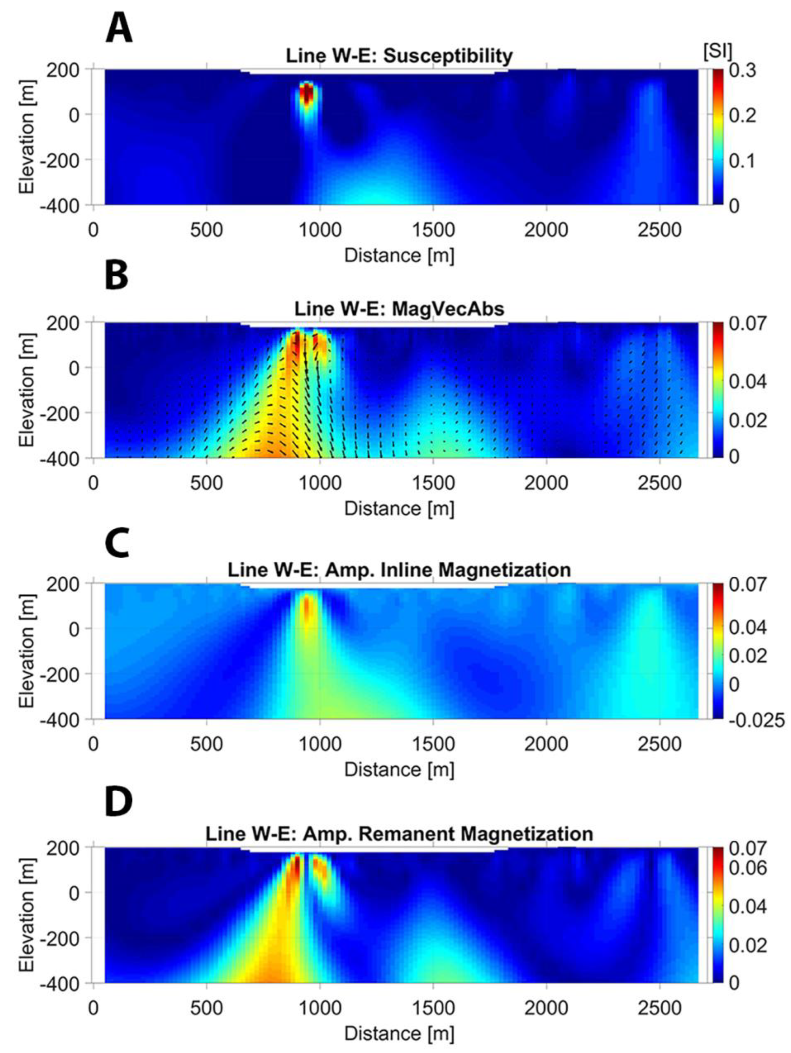
Figure 10 illustrates the W–E profiles of the magnetic models. While the susceptibility model identifies a high susceptibility anomaly near the surface, the magnetization vector models provide a more detailed structure. Specifically, there is a subvertical feature directly west of the susceptibility anomaly at a depth of several hundred meters.
9.2. Comparison of the Inversion Results Using TMI and FTMG Data
Figure 11, Figure 12 and Figure 13 compare the S–N profiles of the susceptibility, inline, and remanent magnetization models, respectively, inverted using the FTMG data and the TMI data which were computed using the tensor data. One can see that the images produced from FTMG data are more focused and compact and outline the prospective target with better clarity than those generated by inverting the TMI data. We can see the TMI inversions adequately resolve the base of the anomalies; however, the FTMG inversions provide significantly better resolution in the near surface. The inversion of FTMG data also results in stronger magnetic property contrast between the magnetized formations and the host rocks. Thus, the advantages of using the FTMG data are clear. The improvement in resolution is comparable to that of airborne gravity gradiometry (AGG) over the vertical gravity total field [30].
10. Conclusions
We have developed and applied a regularized inversion scheme employing a focusing stabilizer and Gramian constraints to invert FTMG data. We have also introduced a new approach to determining the remanent magnetization from the magnetic field and magnetic gradiometry data. These new methods were applied to the airborne magnetic and magnetic gradiometry survey data acquired in the Thompson Nickel Belt. The significant ultramafic formation in the region is distinctly visible in the data, and the surrounding lithologies are also directly imaged in the remanent magnetization transformation of the full magnetization vector. This technique provides a more comprehensive view of the geology and mineralization of the surveyed region. The study has shown the superiority of the inversion of FTMG data over traditional TMI data, as well as the benefits of imaging various components of the magnetization vector.
Author Contributions
Conceptualization, M.S.Z. and M.J.; funding acquisition, B.P. and M.S.Z.; software, M.J.; methodology, M.S.Z. and M.J.; validation, M.S.Z., M.J. and B.P.; investigation, M.J., M.S.Z. and B.P.; writing, M.S.Z. and M.J.; visualization, M.J.; supervision, M.S.Z. All authors have read and agreed to the published version of the manuscript.
Funding
This research was supported by TechnoImaging LLC and Vale Canada Limited and received no external funding.
Data Availability Statement
The data used in this study are not publicly available.
Acknowledgments
We acknowledge the support of TechnoImaging LLC, and CEMI, University of Utah. In addition, we thank Dias Airborne for providing good-quality data and Vale Canada Limited for permission to publish.
Conflicts of Interest
The authors declare no conflict of interest.
Appendix A
The RRCG Algorithm for Solving the Inverse Problem in the Log Space of the Model Parameters
Let us define the forward operator and the corresponding Fréchet derivative in the space of the logarithmic model parameters as Al and Fl. It is easy to see that the following relationship takes place:
We take a derivative of Equation (A1) with respect to m on both sides:
Equation (A2) can be simplified as follows:
where is the Fréchet derivative in the space of original model parameters. In the case of a linear operator, F = A.
One can use Formula (A3) to calculate the Fréchet derivative in the space of the logarithmic model parameters if is known.
From Equation (62), we find
We can write the last equation using the matrix notation:
By substituting Equation (A5) into Equation (A3), we find
Equation (A6) makes it possible to find the Fréchet derivative in the space of the logarithmic model parameters directly if we know the Fréchet derivative in the original space.
In the space of the logarithmic model parameters, the Tikhonov parametric functional can be written as follows:
Here
and
In Equation (A7), the misfit part can be calculated in the original model space instead of the space of logarithmic model parameters since identity (A1) takes place.
Again, let us set
and
Then, Equation (A7) can be rewritten in the space of the weighted model parameters as follows:
The algorithm for re-weighted regularized conjugate gradient minimization of parametric functional (A10) in the space of the weighted logarithmic model parameters can be described as follows:
, if , and , if .
The above iteration process is terminated when the misfit reaches the given level :
References
- Stolz, R.; Zakosarenko, V.; Schulz, M.; Chwala, A.; Fritzsch, L.; Meyer, H.G.; Kostlin, E.O. Magnetic full-tensor SQUID gradiometer system for geophysical applications. Lead. Edge 2006, 25, 178–180. [Google Scholar] [CrossRef]
- Stolz, R.; Schiffler, M.; Zakosarenko, V.; Larnier, H.; Rudd, J.; Chubak, G.; Polomé, L.; Pitts, B.; Schneider, M.; Schulz, M.; et al. Status and future perspectives of airborne magnetic gradiometry. In SEG Technical Program Expanded Abstracts 2011, Proceedings of the IMAGE Annual Meeting, Denver, CO, USA, 26 September–1 October 2021; Society of Exploration Geophysicists: Tulsa, OK, USA, 2021. [Google Scholar]
- Stolz, R.; Schiffler, M.; Becken, M.; Thiede, A.; Schneider, M.; Chubak, G.; Marsden, P.; Bergshjorth, A.B.; Schaefer, M.; Terblanche, O. SQUIDs for magnetic and electromagnetic methods in mineral exploration. Miner. Econ. 2022, 35, 467–494. [Google Scholar] [CrossRef]
- Queitsch, M.; Schiffler, M.; Stolz, R.; Rolf, C.; Meyer, M.; Kukowski, N. Investigation of three-dimensional magnetization of a dolerite intrusion using airborne full tensor magnetic gradiometry (FTMG) data. Geophys. J. Int. 2019, 217, 1643–1655. [Google Scholar]
- Jorgensen, M.; Zhdanov, M.S.; Parsons, B. 3D inversion of QMAGT airborne magnetic gradiometry data for susceptibility and magnetization vector models of the Thompson Nickel Belt in Manitoba, Canada. In SEG Technical Program Expanded Abstracts 2022, Proceedings of IMAGE Annual Meeting, Houston, TX, USA, 28 August–1 September 2022; Society of Exploration Geophysicists: Tulsa, OK, USA, 2022. [Google Scholar]
- Zhdanov, M.S.; Cai, H.; Wilson, G.A. 3D inversion of full tensor magnetic gradiometry (FTMG) data. In SEG Technical Program Expanded Abstracts 2011, Proceedings of SEG Annual Meeting, San Antonio, TX, USA, 18 September–23 September 2011; Society of Exploration Geophysicists: Tulsa, OK, USA, 2011. [Google Scholar]
- Zhdanov, M.S.; Cai, H.; Wilson, G.A. 3D inversion of SQUID magnetic tensor data. J. Geol. Geosci. 2012, 1, 1000104. [Google Scholar]
- Cuma, M.; Wilson, G.A.; Zhdanov, M.S. Large-scale 3D inversion of potential field data. Geophys. Prospect. 2012, 60, 1186–1199. [Google Scholar] [CrossRef]
- Cuma, M.; Zhdanov, M.S. Massively parallel regularized 3D inversion of potential fields on CPUs and GPUs. Comput. Geosci. 2014, 62, 80–87. [Google Scholar] [CrossRef]
- Zhdanov, M.S. Geophysical Inverse Theory and Regularization Problems; Elsevier: Waltham, MA, USA, 2002. [Google Scholar]
- Bhattacharyya, B.K. A generalized multibody model for inversion of magnetic anomalies. Geophysics 1980, 45, 255–270. [Google Scholar] [CrossRef]
- Zhdanov, M.S. Geophysical Electromagnetic Theory and Methods; Elsevier: Waltham, MA, USA, 2009. [Google Scholar]
- Cai, H. Migration and Inversion of Magnetic and Magnetic Gradiometry Data. Master’s Thesis, The University of Utah, Salt Lake City, UT, USA, 2012. [Google Scholar]
- Lelièvre, P.G.; Oldenburg, D.W. A 3D total magnetization inversion applicable when significant, complicated remanence is present. Geophysics 2009, 74, L21–L30. [Google Scholar] [CrossRef]
- Jorgensen, M.; Zhdanov, M.S. Recovering magnetization of rock formations by jointly inverting airborne gravity gradiometry and total magnetic intensity data. Minerals 2021, 11, 366. [Google Scholar] [CrossRef]
- Koenigsberger, J.G. Natural residual magnetism of eruptive rocks. Terr. Magn. Atmos. Electr. 1938, 43, 299–320. [Google Scholar] [CrossRef]
- Clark, D.A.; Emerson, D.W. Notes on rock magnetization characteristics in applied geophysical studies. Explor. Geophys. 1991, 22, 547–555. [Google Scholar] [CrossRef]
- Zhdanov, M.S. Inverse Theory and Applications in Geophysics; Elsevier: Waltham, MA, USA, 2015. [Google Scholar]
- Mehanee, S.; Golubev, N.; Zhdanov, M. Weighted regularized inversion of magnetotelluric data. In SEG Technical Program Expanded Abstracts 1998, Proceedings of SEG Annual Meeting, New Orleans, LA, USA, 8 November–13 November 1998; Society of Exploration Geophysicists: Tulsa, OK, USA, 1998. [Google Scholar]
- Zhdanov, M.; Hursan, G. 3D electromagnetic inversion based on quasi-analytical approximation. Inverse Probl. 2000, 16, 1297. [Google Scholar] [CrossRef]
- Li, Y.; Oldenburg, D.W. Joint inversion of surface and three-component borehole magnetic data. Geophysics 2000, 65, 540–552. [Google Scholar] [CrossRef]
- Li, Y.; Oldenburg, D.W. 3-D inversion of magnetic data. Geophysics 1996, 61, 394–408. [Google Scholar] [CrossRef]
- Portniaguine, O.; Zhdanov, M.S. Focusing geophysical inversion images. Geophysics 1999, 64, 874–887. [Google Scholar] [CrossRef] [Green Version]
- Zhu, Y.; Zhdanov, M.S.; Čuma, M. Inversion of TMI data for the magnetization vector using Gramian constraints. In SEG Technical Program Expanded Abstracts 2015, Proceedings of SEG Annual Meeting, New Orleans, LA, USA, 18 October–23 October 2015; Society of Exploration Geophysicists: Tulsa, OK, USA, 2015. [Google Scholar]
- Zhdanov, M.S.; Gribenko, A.V.; Wilson, G. Generalized joint inversion of multimodal geophysical data using Gramian constraints. Geophys. Res. Lett. 2012, 39, 15482846. [Google Scholar] [CrossRef] [Green Version]
- Cox, L.H.; Zhdanov, M.S. Large-scale 3D inversion of HEM data using a moving footprint. In SEG Technical Program Expanded Abstracts 2007, Proceedings of SEG Annual Meeting, San Antonio, TX, USA, 23–28 September 2007; Society of Exploration Geophysicists: Tulsa, OK, USA, 2007. [Google Scholar]
- Lightfoot, P.C.; Stewart, R.; Gribbin, G.; Mooney, S.J. Relative contribution of magmatic and post-magmatic processes in the genesis of the Thompson Mine Ni-Co sulfide ores, Manitoba, Canada. Ore Geol. Rev. 2017, 83, 258–286. [Google Scholar] [CrossRef]
- Franchuk, A.; Lightfoot, P.C.; Kontak, D.J. High tenor Ni-PGE sulfide mineralization in the South Manasan ultramafic intrusion, Paleoproterozoic Thompson Nickel Belt, Manitoba, Canada. Ore Geol. Rev. 2015, 72, 434–458. [Google Scholar] [CrossRef]
- Zhdanov, M.S. Foundations of Geophysical Electromagnetic Theory and Methods; Elsevier: Waltham, MA, USA, 2018. [Google Scholar]
- Zhdanov, M.S.; Ellis, R.; Mukherjee, S. Three-dimensional regularized focusing inversion of gravity gradient tensor component data. Geophysics 2004, 69, 925–937. [Google Scholar] [CrossRef]
Figure 1.
Graphic representation of magnetization vector M behavior in different rock types. The purple arrow represents the magnetization vector in the presence of remanence.
Figure 1.
Graphic representation of magnetization vector M behavior in different rock types. The purple arrow represents the magnetization vector in the presence of remanence.

Figure 2.
Synthetic model study: comparison of inversion of TMI and FTMG data for magnetic susceptibility and magnetization vector. Panel (A) shows the vertical section of the actual magnetization model. Panel (B) presents the susceptibility model obtained from the inversion of the synthetic TMI data. Panel (C) shows the susceptibility model obtained from the inversion of synthetic FTMG data. Finally, panel (D) shows with the white arrows the magnetization vector model obtained from the inversion of synthetic FTMG data. The color map in the background represents the amplitude of this vector. Panels (E,F) show the inline and “remanent” magnetization amplitudes, respectively.

Figure 3.
The digital terrain model (DTM) of the QMAGT survey area is shown in color. The black lines show survey flight lines. The AOI is located near the Ospwagan Group, indicated by the purple in the inset map of Manitoba, shown on the top left side of the figure. The inserted map is after [28]. The black arrows show the location of profiles S–N and W–E.

Figure 4.
The maps of components of the observed and predicted FTMG data from the magnetization vector inversion. All components have a similar level of data misfit, less than 10%.
Figure 4.
The maps of components of the observed and predicted FTMG data from the magnetization vector inversion. All components have a similar level of data misfit, less than 10%.

Figure 5.
3D isobody view of inverted susceptibility model with values over 0.1 SI shown in green.

Figure 6.
3D isobody view of inverted inline magnetization model with values over 0.02 shown in yellow.
Figure 6.
3D isobody view of inverted inline magnetization model with values over 0.02 shown in yellow.

Figure 7.
3D isobody view of inverted remanent magnetization model with values over 0.04 shown in red.
Figure 7.
3D isobody view of inverted remanent magnetization model with values over 0.04 shown in red.

Figure 8.
Composite 3D isobody view of inverted magnetic models. The mystery ultramafic intrusion is shown in yellow and green. The potential breccia-associated mineralization is shown in red.
Figure 8.
Composite 3D isobody view of inverted magnetic models. The mystery ultramafic intrusion is shown in yellow and green. The potential breccia-associated mineralization is shown in red.

Figure 9.
Line S–N profiles of the inverted magnetic models. Panel (A) shows the magnetic susceptibility model. Panel (B) shows the amplitude of the magnetization vector in color with the projection of the full magnetization vector shown by the black arrows. Panels (C,D) show the inline and remanent components of the magnetization vector, respectively.

Figure 10.
Line W–E profiles of the inverted magnetic models. Panel (A) shows the magnetic susceptibility model. Panel (B) shows the amplitude of the magnetization vector in color with the projection of the full magnetization vector shown with the black arrows. Panels (C,D) show the inline component and remanent component of the magnetization vector, respectively.

Figure 11.
Comparison of the susceptibility models inverted using the FTMG data (Panel (A)) and the computed TMI data (Panel (B)).
Figure 11.
Comparison of the susceptibility models inverted using the FTMG data (Panel (A)) and the computed TMI data (Panel (B)).

Figure 12.
Comparison of the inline magnetization models inverted using the FTMG data (Panel (A)) and the computed TMI data (Panel (B)).
Figure 12.
Comparison of the inline magnetization models inverted using the FTMG data (Panel (A)) and the computed TMI data (Panel (B)).

Figure 13.
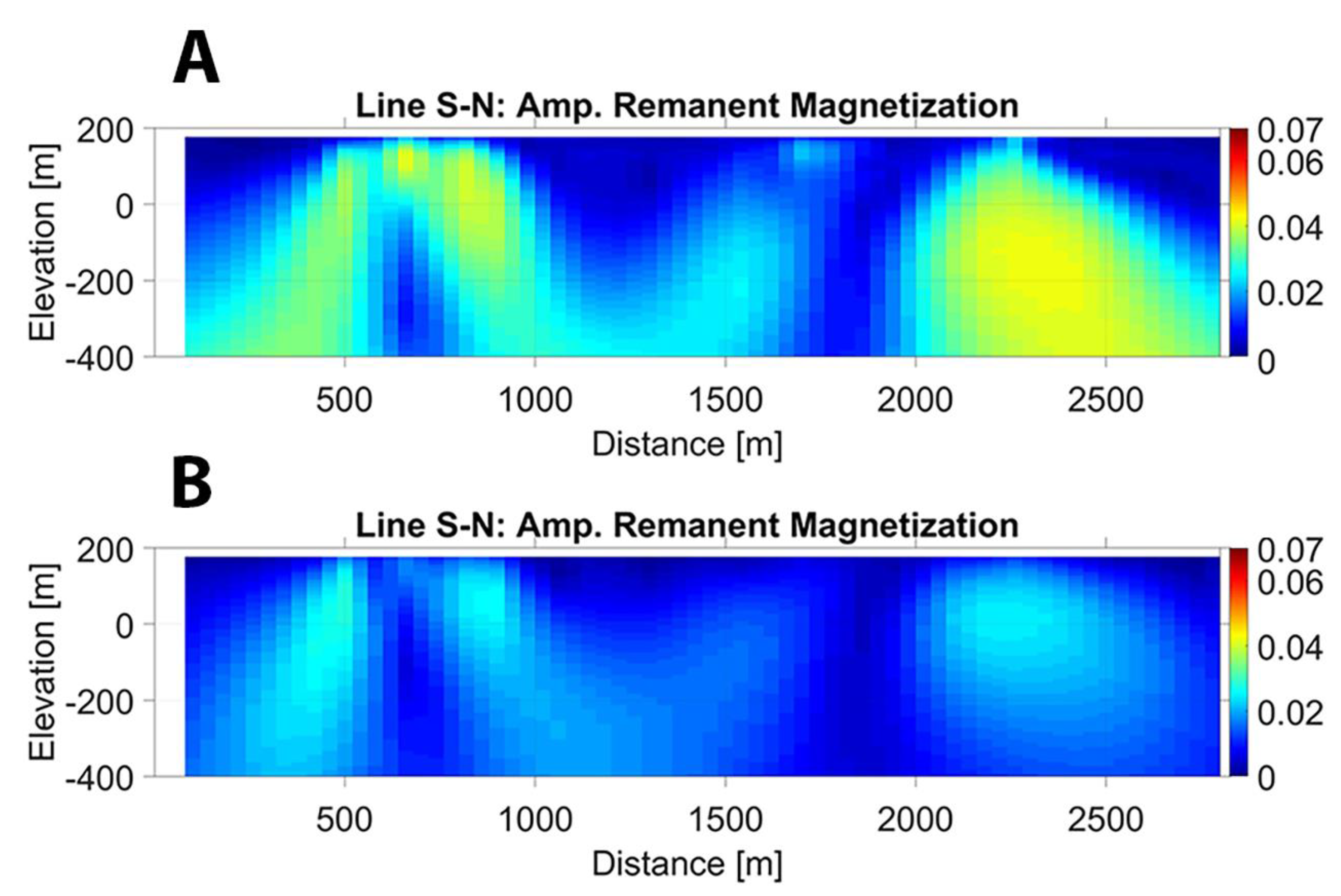
Comparison of the remanent magnetization models inverted using the FTMG data (Panel (A)) and the computed TMI data (Panel (B)).
Figure 13.
Comparison of the remanent magnetization models inverted using the FTMG data (Panel (A)) and the computed TMI data (Panel (B)).

Disclaimer/Publisher’s Note: The statements, opinions and data contained in all publications are solely those of the individual author(s) and contributor(s) and not of MDPI and/or the editor(s). MDPI and/or the editor(s) disclaim responsibility for any injury to people or property resulting from any ideas, methods, instructions or products referred to in the content. |
© 2023 by the authors. Licensee MDPI, Basel, Switzerland. This article is an open access article distributed under the terms and conditions of the Creative Commons Attribution (CC BY) license (https://creativecommons.org/licenses/by/4.0/).
Share and Cite
MDPI and ACS Style
Jorgensen, M.; Zhdanov, M.S.; Parsons, B. 3D Focusing Inversion of Full Tensor Magnetic Gradiometry Data with Gramian Regularization. Minerals 2023, 13, 851. https://0-doi-org.brum.beds.ac.uk/10.3390/min13070851
AMA Style
Jorgensen M, Zhdanov MS, Parsons B. 3D Focusing Inversion of Full Tensor Magnetic Gradiometry Data with Gramian Regularization. Minerals. 2023; 13(7):851. https://0-doi-org.brum.beds.ac.uk/10.3390/min13070851
Chicago/Turabian StyleJorgensen, Michael, Michael S. Zhdanov, and Brian Parsons. 2023. "3D Focusing Inversion of Full Tensor Magnetic Gradiometry Data with Gramian Regularization" Minerals 13, no. 7: 851. https://0-doi-org.brum.beds.ac.uk/10.3390/min13070851
Note that from the first issue of 2016, this journal uses article numbers instead of page numbers. See further details here.