Resource and Reserve Calculation in Seam-Shaped Mineral Deposits; A New Approach: “The Pentahedral Method”

Abstract

In recent years, the introduction of specific software for the evaluation of geological resources and mineral reserves has increased significantly thanks to the use of block models capable of working with large databases and applicable to virtually all types of deposits. It is only in layered, tabular-shaped deposits where the use of block models poses certain drawbacks, not only in terms of visual representation but also during the process of interpolation. Other calculation methods for tabular bodies such as sections, polygons, and triangles work with 2D projections but not with 3D. The “Pentahedral” method described here is undoubtedly an innovative method that allows work to always be conducted in 3D, providing a fairly accurate representation of tabular bodies and making it possible to carry out calculations of resources and reserves using any interpolation method. It is demonstrated with figures and tables of the Carlés mineral deposit, a well-developed exoskarn gold deposit in northwestern Spain (Asturias) where the authors have worked extensively. The pentahedral method takes into account not only geological and stratigraphic data from the model interpolation, but also mining concepts such as “minimum thickness” related to the minimum seam size that can be economically and technically mined, and “overbreak” related to the dilution effect that appears during the mining process due to over-excavation.

1. Introduction

Once the geological, geochemical, and structural information of a mineral deposit are known, it must be represented in 3D in order to obtain sufficiently accurate estimates of its mineralogical content [1], which will lead to the estimation of both mineral resources and mineral reserves, as is explained in international standards such as those from the Canadian Institute of Mining, Metallurgy and Petroleum (CIM) [2].

According to CIM standards, a Mineral Reserve is the economically mineable part of a Measured or Indicated Mineral Resource demonstrated by at least a Preliminary Feasibility Study. This study must include adequate information on mining, processing, metallurgical, economic, and other relevant factors that demonstrate, at the time of reporting, that economic extraction can be justified. A Mineral Reserve includes diluting materials and allowances for losses that may occur when the material is mined.

Despite the existence of several resource estimation methodologies [3], from traditional to geostatistical ones [4,5,6] that use the block model as a geometrical representation, in the particular case of tabular or seam-shaped deposits these methods do not allow a sufficiently accurate representation or interpolation [7].

Hexahedral block models are widely used to simulate and classify resources. Reference [8] shows a study of 120 recent NI 43-101 mineral deposit technical reports, where kriging was the most elaborate one, although used in only seven of the reports. Other more refined methods, such as the sequential indicator simulation (SIS, a pixel-based model) or indicator kriging, are mainly usable in reservoir simulations. Implicit modeling is starting to be implemented in commercial simulation packages, e.g., Leapfrog Radial Basis Functions, Surpac Dynamic Shells Module or Minesight Implicit Modeler, but is recommended for use as an additional tool to provide initial and quick resource analysis, not as a complete replacement of block models [9].

State-of-the-art software uses algorithms that sequentially divide each block into smaller blocks in order to follow the geological structures (sub-blocking), but this approach does not achieve the level of precision required and results in models with an extremely high number of blocks; see [1]. Additionally, sub-blocking uses the composition of the samples surveyed, but does not make an interpolation using the intersections between the surveys and the mineral structure, considering a cutoff, or a minimal thickness, or even considering lateral dilution due to over-excavation. In this paper, it is the “operational mining dilution” that occurs at the time of mining, as defined in [10], which will be referred to as dilution.

Advances have been made in the modeling of local anisotropy in complex geological structures, see [11], but this method does not include mining parameters such as the minimum thickness values or the dilution.

This paper uses a new method to model tabular deposits, as exemplified by the “Zona M” seam of the northern side of the Carlés deposit, in Spain. This deposit is a gold copper skarn, located in the Rio Narcea Gold Belt [12,13,14] formed at the contact between the Carlés granodiorite and the Nieva limestone of the Rañeces Group [15,16]. It consists of several seam-shaped mineral bodies, some of them with economical grades of Au and Cu, with thicknesses ranging from 1 to 6 m and dips from 40° in the north (55°) direction (eastern areas) to 70° in the north (30°) direction (northern bodies).

In the Carlés deposit there are several seams, each of them continuous. They are separated by faults or are located in different contact areas. As is standard practice in classical block models, bodies or seams divided by faults should be treated as different bodies and studied separately.

RECMIN (from: “REC ursos MIN eros” which translates as “mineral resources” in English) software will be used throughout the research in order to manage data and visualization; see [17]. RecMin is free software used in mineral deposit modeling, developed entirely by the authors over the past 25 years and thoroughly tested in real working conditions at dozens of mining projects.

RecMin code was supplemented with enough algorithms to consider this new calculation method, described further on.

This paper will show how to work with calculation units geometrically different from blocks. The pentahedral method also adds information usually not taken into account in block modeling, such as “lateral dilution” or “mining intercept”.

2. Research Objectives

The main goal of this research is the evaluation of the seam-shaped mineralized structure using a new methodology that provides a precise representation of morphology and physical and chemical characteristics, and storing this information in a suitable manner in order to proceed with resource estimations. The specific objectives of the method are:

• Three-dimensional (3D) modeling is mandatory;
• It must allow different interpolation algorithms, including geostatistics;
• The calculation detail has to be user-defined;
• Dilution (material below the cutoff) should be considered, if necessary;
• It must allow estimates with a categorization using distances, number of intercepts, or a combination of both parameters;
• It must allow interpolation, taking into account boreholes filtered by distance: neighborhood influence;
• The results will be stored in a Structured Query Language (SQL) database.

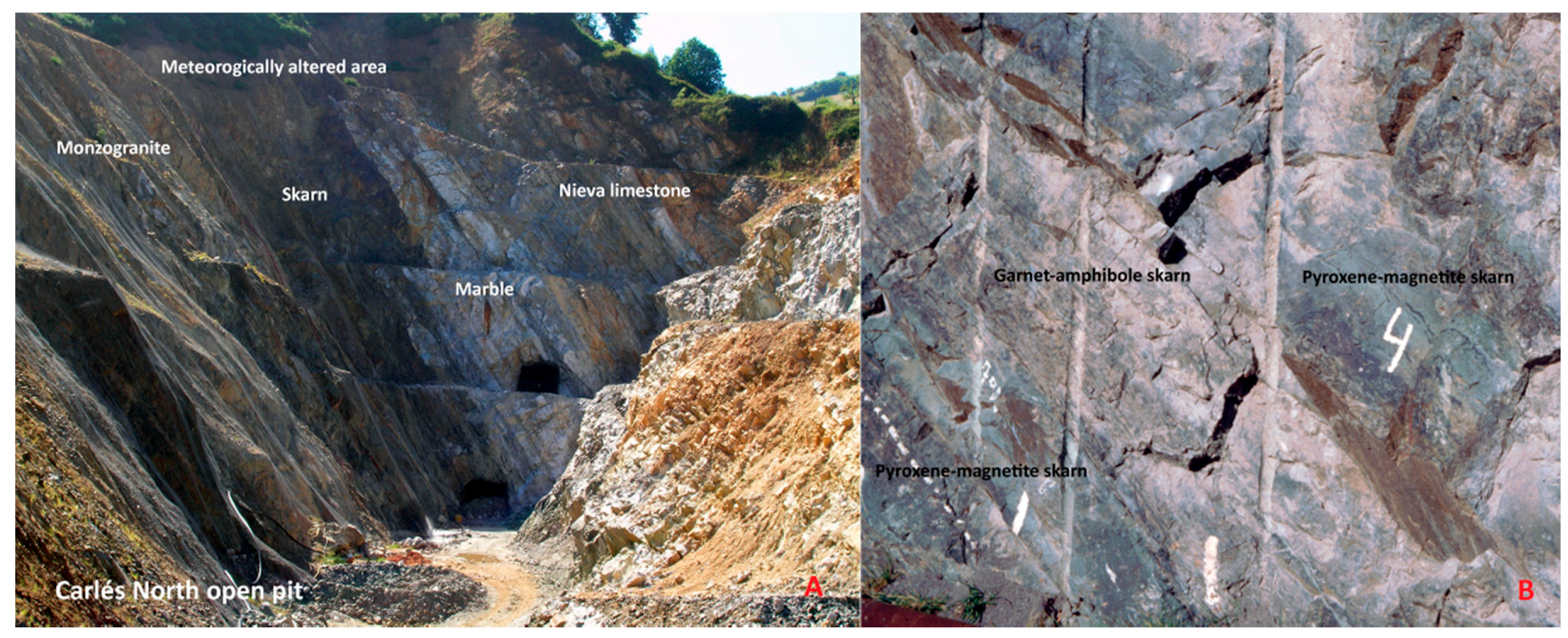
3. Geological Characteristics and Constraints

The Carlés Cu-Mo-Au ore deposit is located in the Rio Narcea Gold Belt (RNGB), in the Cantabrian zone of the Iberian Massif. It is related to a small postkinematic calcalkaline monzogranite, which intrudes as a cedar tree laccolith into the upper siliciclastic Furada Formation (shales, oolitic ironstones, and, at the top, some carbonate layers of late Silurian age) and the Nieva carbonates (mostly limestones and some dolostones of early Devonian age), developing skarns bearing copper, molybdenum, and gold of economic interest (Figure 1A).

According to the paper by Martin-Izard et al. [16], the Carlés deposit consists mainly of a well-developed exoskarn [18]. The Carlés intrusive is a monzogranite, up to 800 m in diameter, which intrudes along the contact of a Silurian siliciclastic formation and a Devonian carbonate formation. It is a light gray, medium-grained, equigranular igneous rock with plagioclase, biotite, quartz, K-feldspar, and magnesiohornblende. The accessory minerals are zircon, rutile, ilmenite, magnetite, and apatite. The plagioclase (An 30–47) has normal zoning with a common narrow albite-oligoclase (An 8–20) rim. The skarn is at the contact between the monzogranite and the carbonate rock, where a Cu-Au-Mo calcic skarn developed. The mineralized area is divided into three main sectors (east, west and north sectors; See Figure 1), all of which have been studied by Martin-Izard et al. [13]. At the moment the east and north sectors are being exploited (Figure 1A–C), both by open pit and also by underground mining.

The exoskarn is mostly calcic skarn made up of early garnet and pyroxene, and later amphibole, magnetite, and sulfides (Figure 2A,B). The ore is related to the skarn retrogradation and post-skarn veining and faulting.

The metasomatic phenomena give way to alternating layers, centimeters to meters in thickness, of garnet-dominant and pyroxene-dominant skarn. Retrograde alteration of the garnet-pyroxene skarn to form a pyroxene, amphibole, magnetite and sulfide minerals assemblage is a very important process in the Carlés deposit. Above all, metallic mineralization at Carlés is most important in lenses within amphibole-pyroxene bands.

4. Methodology

“Zona M” in the northern area of the Carlés deposit is the zone this study will focus on. The calculation procedure was developed in the following phases:

• Determination of the seam localization from the geological information and survey data.
• Construction of a 3D-modeled surface at the center of the seam.
• Generation of an equally-spaced cloud of points in the seam centered surface.
• Calculation of the intercept values of the surveys crossing the seam.
• Execution of a geostatistical study of the intercept values.
• Interpolation of the grade and the thickness of each point of the cloud of points, using the intercept information.
• Definition of the estimation categories and generation of the calculation units.
• Database generation and representation.

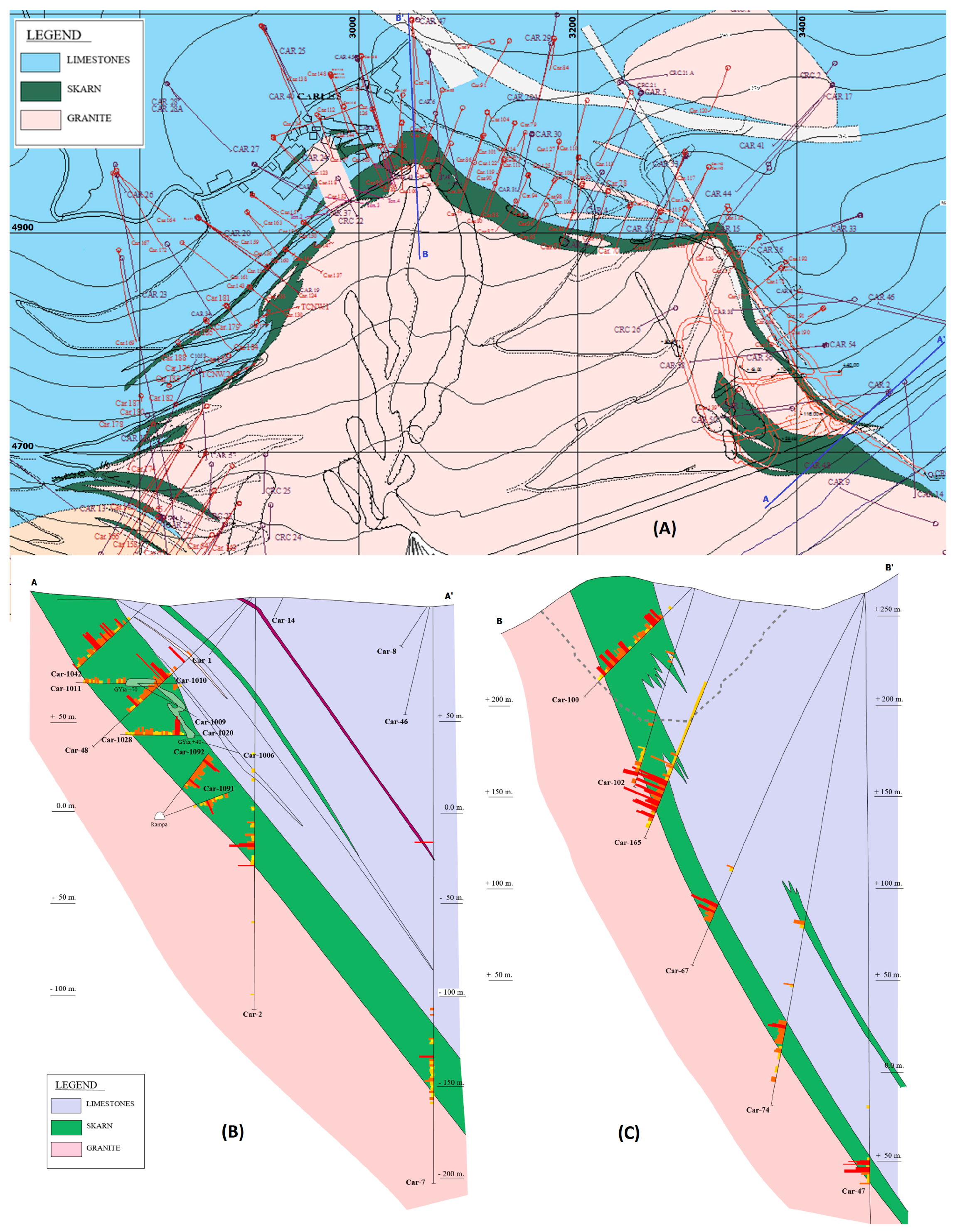
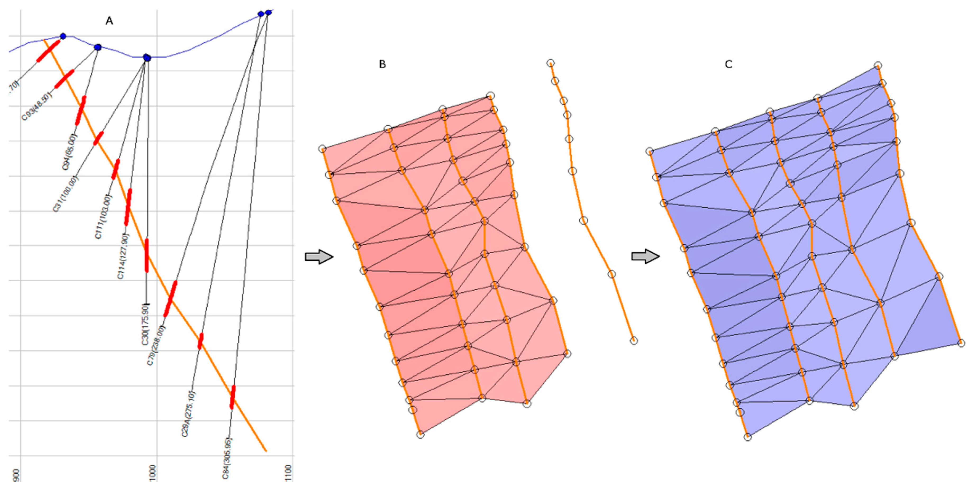
4.1. Determination of the Seam Localization from the Geological Information and Surveys

For each and every borehole, the intercept interval of the “ZONA M” mineralized body was determined, without considering the grade value, only considering the skarn lithology.

The seam localization has to be broad enough to allow late adjustments as the modeling defines the correct economical limits, from parameters such as cutoff grade, minimal thickness, or lateral dilution. Figure 3 shows graphically the seam limits at a borehole intercept and the associated bar chart displaying grade data.

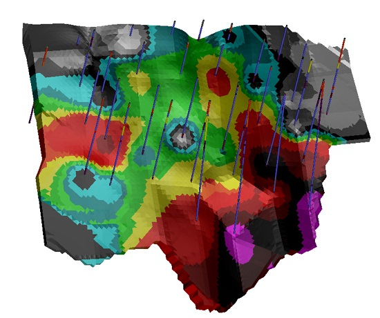
4.2. Construction of a 3D Modeled Surface at the Center of the Seam

As stated above, once the borehole intervals that intercept the mineralized body have been defined, a surface at the center of this body has to be created, from where the interpolation point mesh will be created. As noted above, the surface does not need to be located exactly, as the software will adjust its final position according to the real values of the borehole intercepts and the body.

The easiest way to proceed is to work section by section (Figure 4). Figure 4A shows a cross section of boreholes depicted in white whereas the intercepts with the body are depicted in red. The green line connects the centers of each red line section. Figure 4B simultaneously shows several sections and their corresponding centerlines, which are triangulated to generate a surface. Figure 4C shows the final calculated surface, which will henceforth be referred to as “T1”.

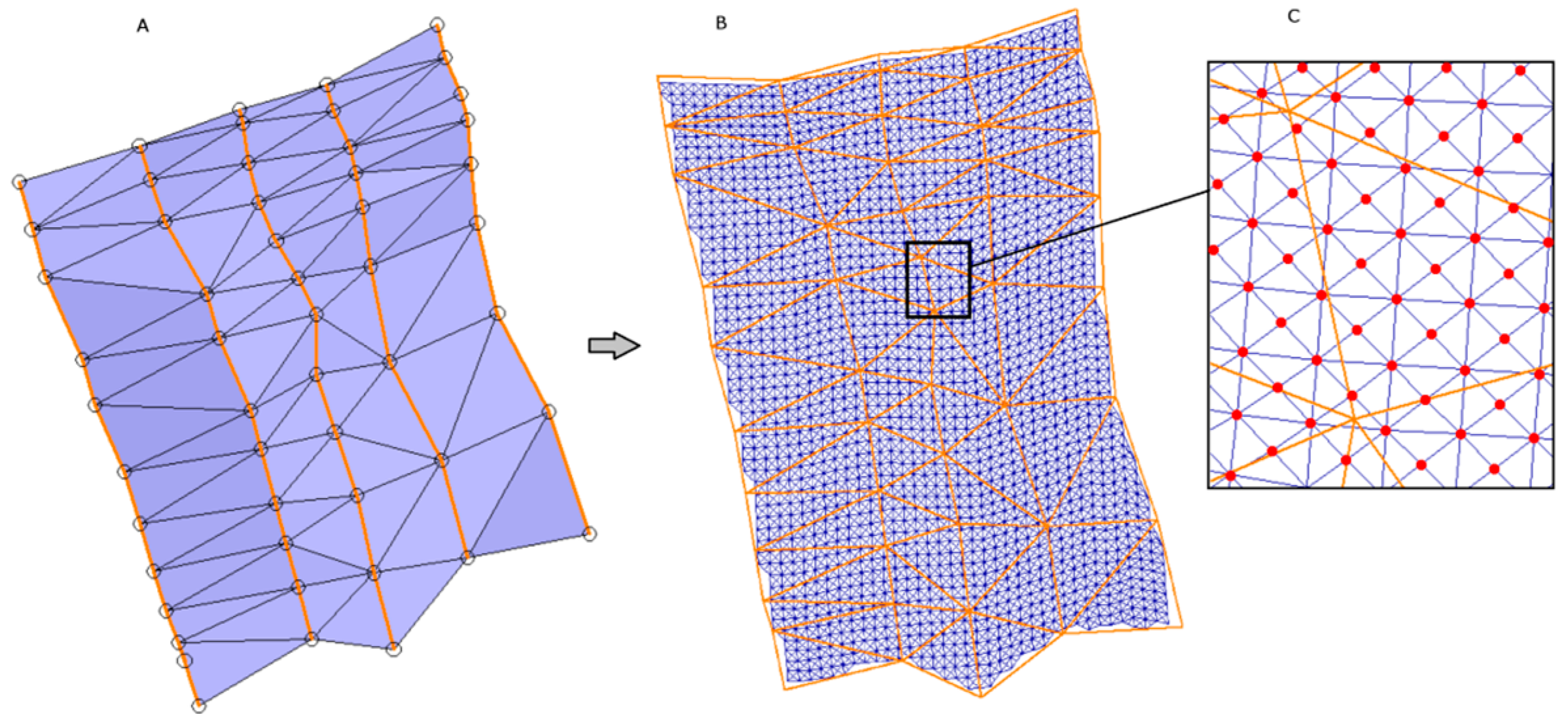
4.3. Generation of an Equally Spaced Cloud of Points in the Seam Centered Surface

In order to have equally spaced interpolation points over the T1 surface, T1 will be remeshed to generate T2, with a point density high enough to reflect geology variation. A high point density will not alter the resource calculations, as interpolation points too close to each other will display the same results as if they were close to the intercepts. This cloud of points will be referred to as NPS from now onwards. The software will automatically cut parallel sections of T1 at a defined distance (5 m in this example, as the borehole density is 25 × 25 and 5 intermediate points between boreholes have been considered) in a selected direction (the X axis in this example). Inside each line generated by each cut, points are defined by a certain distance, user-selectable (5 m again in this example) on the perpendicular axis (Y in this case). Note that 5 m is a suitable value in the case of the “ZONA M” ore body. This value has to be adjusted according to each ore body size and morphology so as to obtain the necessary accuracy for mining the resource, see [7].

Once the evenly spaced cloud of points is generated (Cartesian mesh), the software will create new points at the cross of the diagonals connecting any four points of each generated square (Figure 5C). Figure 5B shows the outcome of this operation. Finally, the algorithm will create triangles that mimic the seam-centered surface. This triangulated surface will be called T2.

All the information is stored in a database (BDS), previously created in the database.

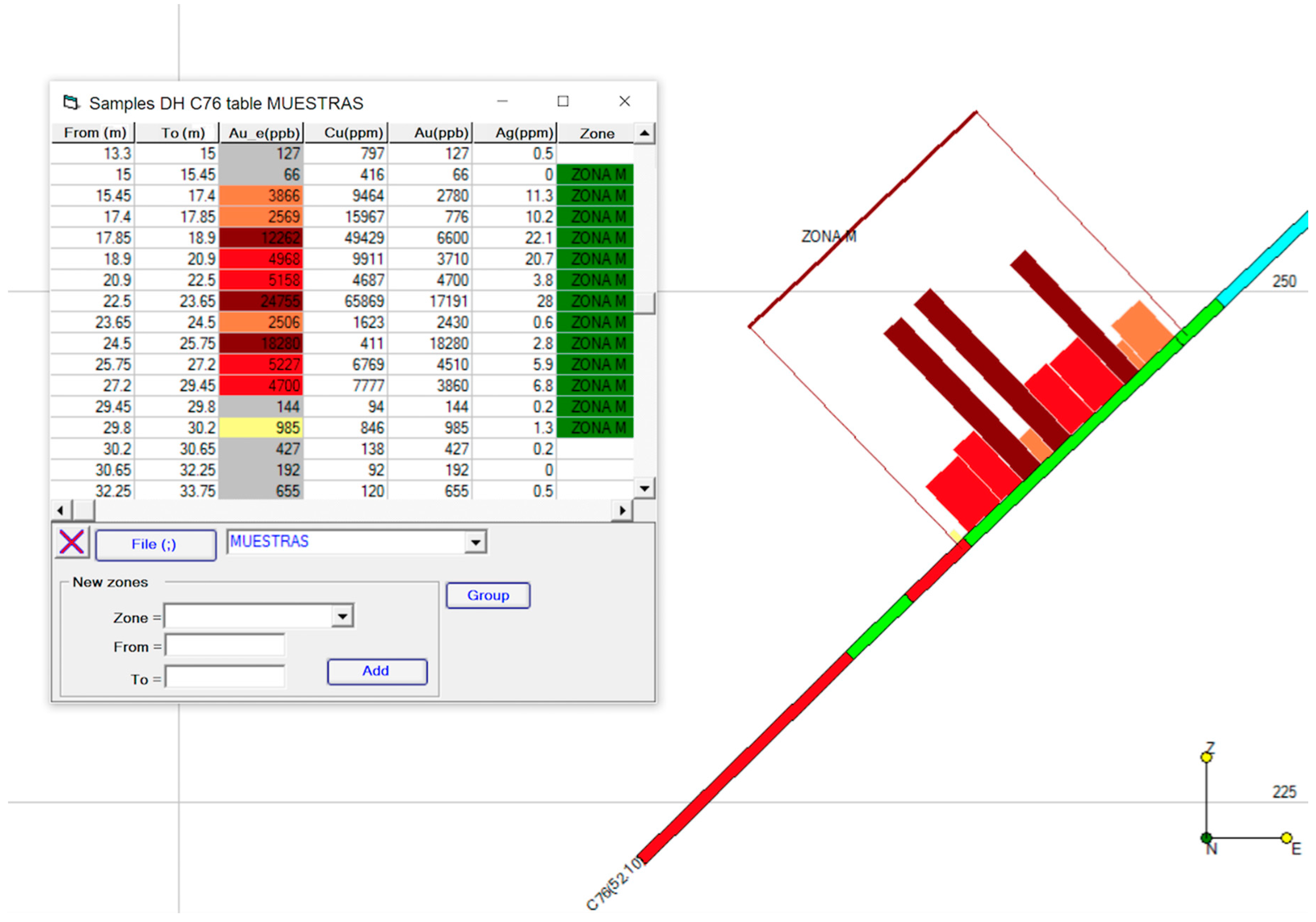
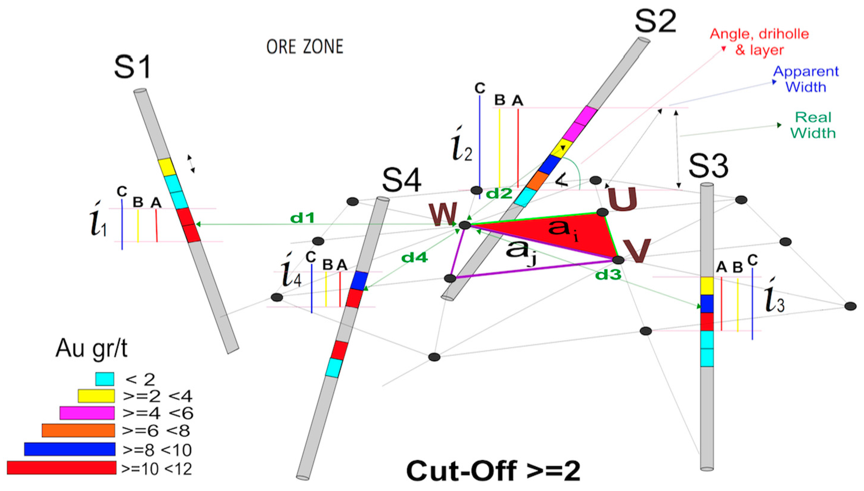
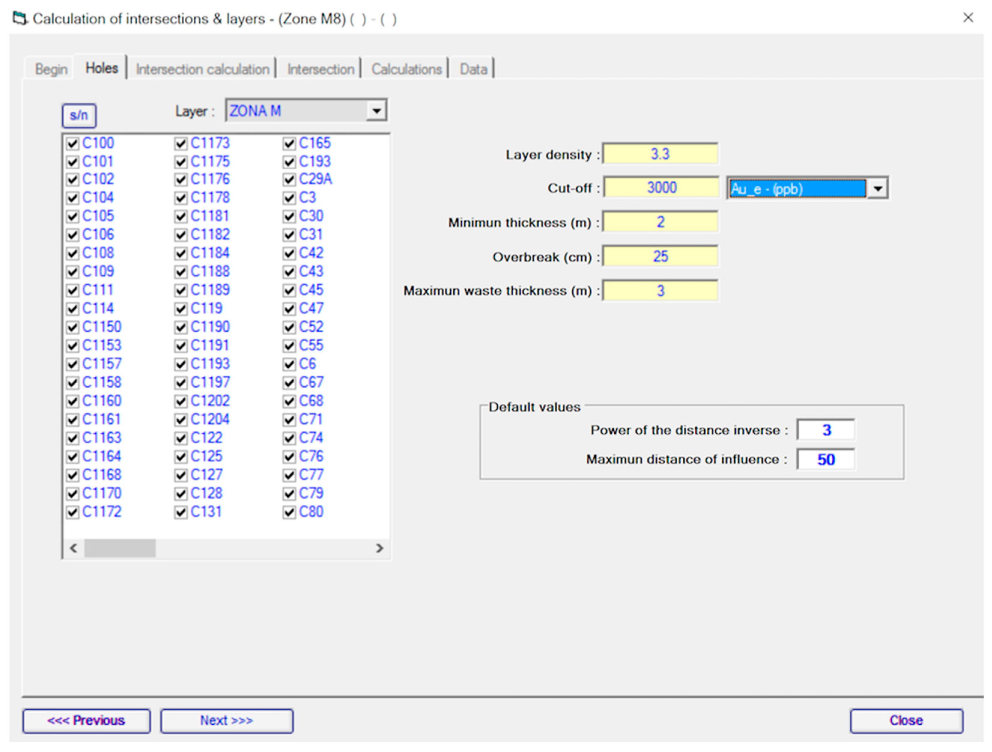
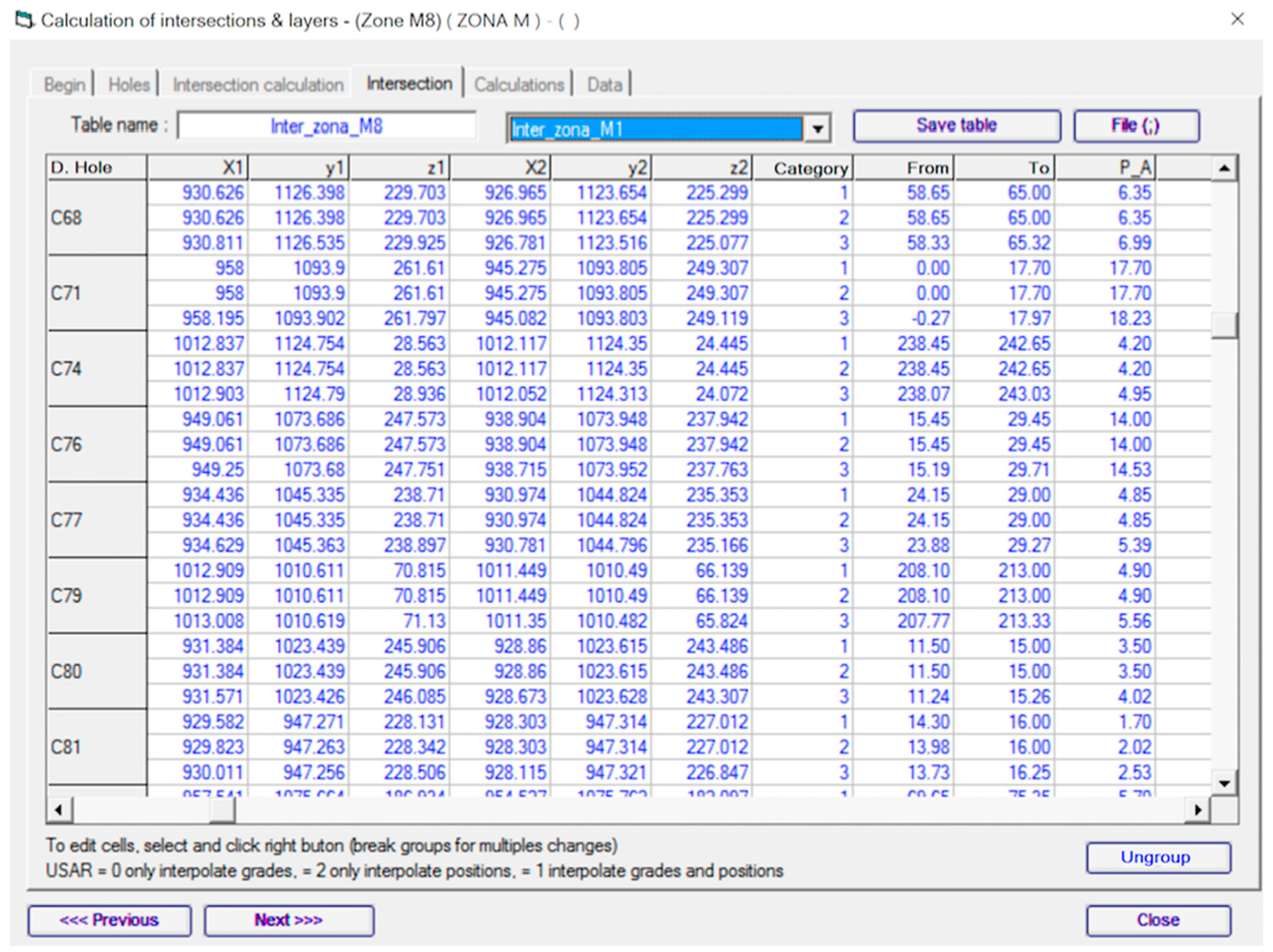
4.4. Calculation of the Intercept Values of the Surveys Crossing the Seam

Before the interpolation of grades and thicknesses at each point of the NPS, the economical interval in each borehole (intercept) must be calculated.

Cutoff grade. This is defined as the minimum grade that allows economical exploitation of the ore body, see [19]. In the example that is being used, the “Zona M” ore body of the Carlés deposit hosts three recoverable elements: Au, Cu, and Ag. A new element called “Au_e” element or “Au grade equivalent” can be defined, where an accumulated value of the three elements is stored according to a price-weighting index scheme. In order to simplify the calculation, an average metal recovery value was assumed, understood as the final percentage of each metal that gives a monetary income, deducting the concentration plant recovery, selling costs, concentration transport, penalties, besides other factors.

Minimum thickness. A minimum value of seam thickness must be considered in order to reflect the economic feasibility of the exploitation. It depends on the rock type, the seam dip and the mining method (room and pillar, sublevel stopping, cut and fill). A thickness of 2 m has been considered in this example, according to the mining machinery size that can be used in this deposit mining.

Mining overbreak. A lateral dilution has been defined due to unwanted results of blasting and hole deviations. From our experience with this deposit, 50 cm of overbreak (overexcavation, 25 cm each side) is defined, a value that can be user-selectable

Maximum thickness of waste rock. A usual situation that is found when the intercept of the borehole and the ore body is calculated is the appearance of inclusions, intervals of waste rock inside the ore body and, more commonly, mineralization below the cutoff grade value. The treatment for this type of situation is achieved by defining a maximum waste thickness value whereby, if the waste thickness value exceeds the maximum, it will not be mined (it will remain as a pillar). If the waste thickness value is calculated to be below the maximum and the average grade is higher than the cutoff grade, it will be considered as ore; however, if the average grade is below the cutoff grade, it will be considered as waste rock and will not be included in the intercept. This maximum waste rock thickness will be referred to as the real thickness of the seam, measured perpendicular to the seam.

The intercept calculation procedure is described below, both graphically and analytically.

In order to explain the procedure of the three intersection types, as well as the interpolation over each point of the NPS, we will refer to four theoretical boreholes: S1, S2, S3, and S4, as represented in Figure 6. The algorithm calculates three different intercepts (denoted as A, B, and C), for each borehole crossing the seam, as follows:

A: Geological Intercept. This includes only those samples with grades higher than the cutoff grade. If there are no samples higher than that value, the highest-grade sample will be defined as the geological intercept. For instance, borehole S2 shows six samples 1 m in size, but only five will be used when considering a cutoff grade of 2 g Au/t, as can be seen in Figure 4 as per the coding colors.

For those samples with grades lower than the cutoff grade being inserted between samples that are above the cutoff grade, the “maximum thickness of waste rock” criteria must be taken into account, as referred to above.

B: Minimum Thickness Intercept. This will be defined as the geological intercept widened as necessary to complete a previously defined minimum real thickness. If the real thickness of the geological intercept is equal to or greater than the minimum thickness value, both intercepts will be the same.

By looking at borehole S2 in Figure 6, and considering 2 m as the minimum thickness value, it can be seen that the geological intercept already has a real thickness of over 2 m, so the minimum thickness intercept (B) will be equal to the geological intercept (A).

If the intercept is less than the minimum thickness, the algorithm will add in samples from the higher grade side. Once the limits are checked, it will re-calculate whether new samples need to be added of a higher cutoff on each side of the intercept.

C: Mining Overbreak Intercept. This will be defined as the minimum real thickness intercept widened at both sides by a distance defined as over excavation. In this example 50 cm will be used (25 cm on each side). This is an important parameter to consider, as it will simulate the mineral dilution that always occurs in common mining procedures that involve excavation.

All three intercepts are calculated referring to real or true thickness; therefore the angle at which the borehole and the seam intercept each other must be known. If the borehole is perpendicular to the seam, this angle is 90° and real and apparent thickness will be equal. This angle, and the intercept point coordinates, is calculated automatically by the algorithm. The intercept point will be the point where the line that represents the borehole cuts one of the triangles of the T2 surface generated from the NPS. The angle will be the one established by the plane of the intersected triangle and the segment representing the borehole.

Nevertheless, the experience of the technician is extremely important in order to define which samples to include in the body. The software allows samples to be accepted or discarded manually in order to refine the calculations. Angles defined by the intersection of boreholes and the seam shaped deposit are calculated at each intersection and can be manually adjusted according to geological knowledge if need be. In this way, possible inaccuracies in apparent thickness calculations are limited.

Interpolation parameters. In this study the Inverse Distance Weighted (IDW) interpolation method will be used; other methods could have been considered: nearest neighbor or kriging, among others. In order to use IDW, a maximum influence distance must be used, calculated through a geostatistical study, independent of the interpolation method shown in this paper and detailed below, as well as a power value. In this case the distance is fixed at 50 m and the power is 3 (Figure 7 shows the input window for these parameters). These values can be different for each intercept, if necessary.

Once the calculation parameters are defined, the software executes the algorithm, which resolves the three intercept types in each borehole that fulfills the defined conditions. This kind of deposit is often high-grade centered, with low-grade values toward the deposit limits. When several high-grade intervals exist over the cutoff grade, the limits for each and every one of the three types of intercepts can be adjusted manually.

Figure 8 is an example of the calculation window. Intercepts are shown as graph bars: red (geological intercept), yellow (minimum thickness intercept) and white (mining overbreak intercept). The x-axis shows samples (“from” and “to” values) and the y-axis shows the different grade values in ppb (parts per billion).

The calculation results (Figure 9) are stored in a database (BDS) that includes three records for each borehole, corresponding to each interpolation type.

4.5. Geostatistical Study of the Intercept Values

As with block model estimation, an influence distance or neighborhood search must be defined. This is necessary in order to consider the quantity and proximity of intercepts to be used in the interpolation and to define the parameters of the classification of the resources or reserves. This is achieved by using a variographic study, which can be performed using a variety of software to which the data must be exported. Several codes are available, both freeware and commercial.

In this example, the data were exported to Stanford Geostatistical Modeling Software (SGEMS), [20], where the variogram was modeled and the main direction and influence distance was found. RecMin can easily export both the composite and/or the intercept data to make this calculation, in both Gslib and Ascii format.

The main direction of the mineralization, as per variogram results, is indicated in graphics by a line parallel to the direction that fits between two of the vertices of the T2 surface (Figure 10). This line is saved as a file and then later selected in the software interpolation assistant in order to be considered as a continuity guide during calculation.

The anisotropy of the variogram is reflected in the different radii of the search ellipsoid. In this case, it is a planar ellipse, as it follows a seam. Both radii of the ellipse, the long and the short, are introduced considering a ratio between them. In this example the ratio is 1:2, with 2 being the secondary direction. Figure 10 shows the shape of the ellipse for a unique theoretical borehole, crossing the seam at the center of the colored sections, as well as the main direction of the mineralization (green line), which follows the main radius of the ellipse.

During the calculation, the vector that connects the intercept and the interpolation point is decomposed in two vectors: one in the main direction and another one in the secondary direction; each vector modulus is multiplied by the corresponding factor as per input data in order to establish the calculation distance.

4.6. Interpolation of the Grade and the Thickness at Each Point of the Cloud of Points (NPS)

In order to understand the interpolation process, please refer to Figure 6 and study the triangle ai with its three vertices U, V, and W. The intercepts are calculated for each vertex with their own influence radius. Assuming that the intercepts of the four boreholes represented in the figure are inside that radius, the following calculations (

Table 1. Calculations worked out for each vertex with their own influence radius.

Borehole S1	Borehole S2	Borehole Sn
A1: Geological Intercept	A2: Geological Intercept	An: Geological Intercept
(L.P)A1: Grade multiplied by thickness	(L.P)A2: Grade multiplied by thickness	(L.P)An: Grade multiplied by thickness
PA1: thickness	PA2: thickness	PAn: thickness
B1: Minimum Thickness Intercept	B2: Minimum Thickness Intercept	Bn: Minimum Thickness Intercept
(L.P)B1: Grade multiplied by thickness	(L.P)B2: Grade multiplied by thickness	(L.P)Bn: Grade multiplied by thickness
PB1: thickness	PB2: thickness	PBn: thickness
C1: Mining Intercept	C2: Mining Intercept	Cn: Mining Intercept
(L.P)C1: Grade multiplied by thickness	(L.P)C2: Grade multiplied by thickness	(L.P)Cn: Grade multiplied by thickness
PC1: thickness	PC2: thickness	PCn: thickness

) are worked out:

The interpolation in case of the vertex W of the triangle a_i will be:

$${\left(L.P\right)}_{WA}=\frac{\frac{{\left(L.P\right)}_{A1}}{d_1^x}+\frac{{\left(L.P\right)}_{A2}}{d_2^x}+\dots +\frac{{\left(L.P\right)}_{An}}{d_n^x}}{{\left(\frac{1}{d_1}\right)}^x+{\left(\frac{1}{d_2}\right)}^x+\dots +{\left(\frac{1}{d_n}\right)}^x}$$

(1)

$$P_{WA}=\frac{\frac{P_{A1}}{d_1^x}+\frac{P_{A2}}{d_2^x}+\dots +\frac{P_{An}}{d_n^x}}{{\left(\frac{1}{d_1}\right)}^x+{\left(\frac{1}{d_2}\right)}^x+\dots +{\left(\frac{1}{d_n}\right)}^x}$$

(2)

$${\left(L.P\right)}_{WB}=\frac{\frac{{\left(L.P\right)}_{B1}}{d_1^x}+\frac{{\left(L.P\right)}_{B2}}{d_2^x}+\dots +\frac{{\left(L.P\right)}_{Bn}}{d_n^x}}{{\left(\frac{1}{d_1}\right)}^x+{\left(\frac{1}{d_2}\right)}^x+\dots +{\left(\frac{1}{d_n}\right)}^x}$$

(3)

$$P_{WB}=\frac{\frac{P_{B1}}{d_1^x}+\frac{P_{B2}}{d_2^x}+\dots +\frac{P_{Bn}}{d_n^x}}{{\left(\frac{1}{d_1}\right)}^x+{\left(\frac{1}{d_2}\right)}^x+\dots +{\left(\frac{1}{d_n}\right)}^x}$$

(4)

$${\left(L.P\right)}_{WC}=\frac{\frac{{\left(L.P\right)}_{C1}}{d_1^x}+\frac{{\left(L.P\right)}_{C2}}{d_2^x}+\dots +\frac{{\left(L.P\right)}_{Cn}}{d_n^x}}{{\left(\frac{1}{d_1}\right)}^x+{\left(\frac{1}{d_2}\right)}^x+\dots +{\left(\frac{1}{d_n}\right)}^x}$$

(5)

$$P_{WC}=\frac{\frac{P_{C1}}{d_1^x}+\frac{P_{C2}}{d_2^x}+\dots +\frac{P_{Cn}}{d_n^x}}{{\left(\frac{1}{d_1}\right)}^x+{\left(\frac{1}{d_2}\right)}^x+\dots +{\left(\frac{1}{d_n}\right)}^x}.$$

(6)

where:

• L: Metal grade, in this case: Au_eq.
• P: Real thickness of the intercept.
• d: Distance between the NPS point to be interpolated and the center of the intercept.
• x: Inverse distance exponent (in the example, x = 3).
• V: Pentahedron volume.
• n: Borehole identification number.
• a: Seam triangle surface.

Notice that the software will interpolate six values per vertex or point of NPS: Grade multiplied by thickness and thickness for each type of intercept. In this case, the four borehole data (S₁, S₂, S₃, and S₄) will be used as they are considered to be inside its area of influence.

The same calculations will be repeated for the U and V vertices as well as for all the points inside the NPS point network over the seam. Then the three average grades of the a_i triangle will be:

$$a_{iA}=\frac{\frac{{\left(L.P\right)}_{WA}}{P_{WA}}+\frac{{\left(L.P\right)}_{UA}}{P_{UA}}+\frac{{\left(L.P\right)}_{VA}}{P_{VA}}}{3}$$

(7)

$$a_{iB}=\frac{\frac{{\left(L.P\right)}_{WB}}{P_{WB}}+\frac{{\left(L.P\right)}_{UB}}{P_{UB}}+\frac{{\left(L.P\right)}_{VB}}{P_{VB}}}{3}$$

(8)

$$a_{iC}=\frac{\frac{{\left(L.P\right)}_{WC}}{P_{WC}}+\frac{{\left(L.P\right)}_{UC}}{P_{UC}}+\frac{{\left(L.P\right)}_{VC}}{P_{VC}}}{3}.$$

(9)

The database will be filled with calculations as shown in

Table 2. Calculation breakdown and interpolation of an NPS triangle.

NPSID	Dist	%	D.Hole	P_R	<Au>	<Ag>	<Cu>	<As>	<Au_e>
30038000070	23.9	36.36%	C1043	1.06	1975	2.4	1200	253	1975.18
30038000070	26.9	25.50%	C1041	0.98	800	0.1	0	3900	800.00
30038000070	30.1	18.20%	C1042	3.03	9992	6.3	5433	15114	9992.76
30038000070	32.4	14.59%	C1012	0.59	2050	0.5	570	1387	2050.08
30038000070	45.3	5.34%	C1089	0.71	4850	8.4	4000	4400	4850.60
30038000070	-	100.00%	-	1.31	3299.1	2.6	1722.1	4275.1	3299.36
30038000060	19.5	59.73%	C1043	1.06	1975	2.4	1200	253	1975.18
30038000060	30.5	15.61%	C1041	0.98	800	0.1	0	3900	800.00
30038000060	34.6	10.69%	C1042	3.03	9992	6.3	5433	15114	9992.76
30038000060	36.5	9.11%	C1012	0.59	2050	0.5	570	1387	2050.08
30038000060	45	4.86%	C1089	0.71	4850	8.4	4000	4400	4850.60
30038000060	-	100.00%	-	1.2	2795.3	2.6	1544	2716.1	2795.57
30038000060	17.4	66.80%	C1043	1.06	1975	2.4	1200	253	1975.18
30038000060	29.5	13.71%	C1041	0.98	800	0.1	0	3900	800.00
30038000060	35.9	7.61%	C1042	0.59	2050	0.5	570	1387	2050.08
30038000060	36.5	7.24%	C1012	3.03	9992	6.3	2533	15114	9992.76
30038000060	42.3	4.65%	C1089	0.71	4850	8.4	4000	4400	4850.60
30038000060	-	100%	-	1.1	2562.8	2.5	1442.1	2158.1	2563.00
TOTAL	-	-	-	1.22	2885.75	2.56	1569.37	3049.37	2885.98

. In this case the vertices have identification numbers (30038000070, 30038500060, and 30039000060). In these intercepts, five boreholes have been included.

The following procedure is applied for attaching a volume to each triangle of T2 and obtaining a volumetric representation of the seam.

In each interpolation point a segment of equal length to the real thickness interpolated at that same point is defined; the direction of this segment will be the average of the directions perpendicular to each of the triangles sharing that point as a vertex and the segment itself will be located so that the interpolation point is at the middle of the segment.

If we connect the ends of the three segments on each corresponding side, two new triangles appear; these triangles, together with the three segments, define a volume that is called the “calculation unit” (Figure 11a).

The volume is calculated by dividing each calculation unit (irregular octahedron) in three irregular tetrahedra, as can be seen in Figure 9b. As the coordinates of each of the four vertices of the irregular tetrahedron are known, its volume can be calculated as shown in Equation (10), where x_i, y_i, z_i are the vertex coordinates:

$$V=\frac{1}{3!}\left|\begin{array}{cccc}{x}_1& y_1& z_1& 1\\ x_2& y_2& z_2& 1\\ x_3& y_3& z_3& 1\\ x_4& y_4& z_4& 1\end{array}\right|$$

(10)

It must be taken into account that each pair of triangles that share an edge will also share the two segments generated at each vertex edge and the corresponding faces of those two triangles will also be the same. In this way, all calculation units match and fill the entire volume that represents the seam (Figure 12).

Finally, the weight will be obtained by multiplying the calculated volume by the seam density for each one of the three calculation types.

Before initiating the calculation, all the parameters are introduced into the software (Figure 13).

4.7. Interpolation of the Positions of the Seam Surface Center

As we have seen in the calculation of intersections, once the calculations are complete and depending on the cutoff grade, minimum thickness or overbreak dilution, the intercept center does not have to match the theoretical center where the borehole cuts the seam center (T1). Differences at these locations will not affect a volume and grade calculation. Nevertheless, it will be of significance if the calculations are going to be used in the planning or exploitation mining phases; the way to correct these positions is by using position interpolation. In this way, the software relocates the center of the seam, moving it depending on how the nearest intercept centers have been moved, and the information is then stored in database fields named MOVX, MOVY, and MOVZ. This procedure relocates the NPS interpolation points by applying the inverse distance weighting method with a certain user-selectable power.

The software can be instructed to store the new point mesh positions in a new table so they can be reused in a subsequent calculation and to obtain graphical representations (Figure 14).

The change in position of the seam center will be the same in the case of “Minimum thickness” and “Mining” interpolations, as they have the same center; in contrast, it will be different in the case of the “Geological” type, so in this case it does not need to be the same, as explained previously.

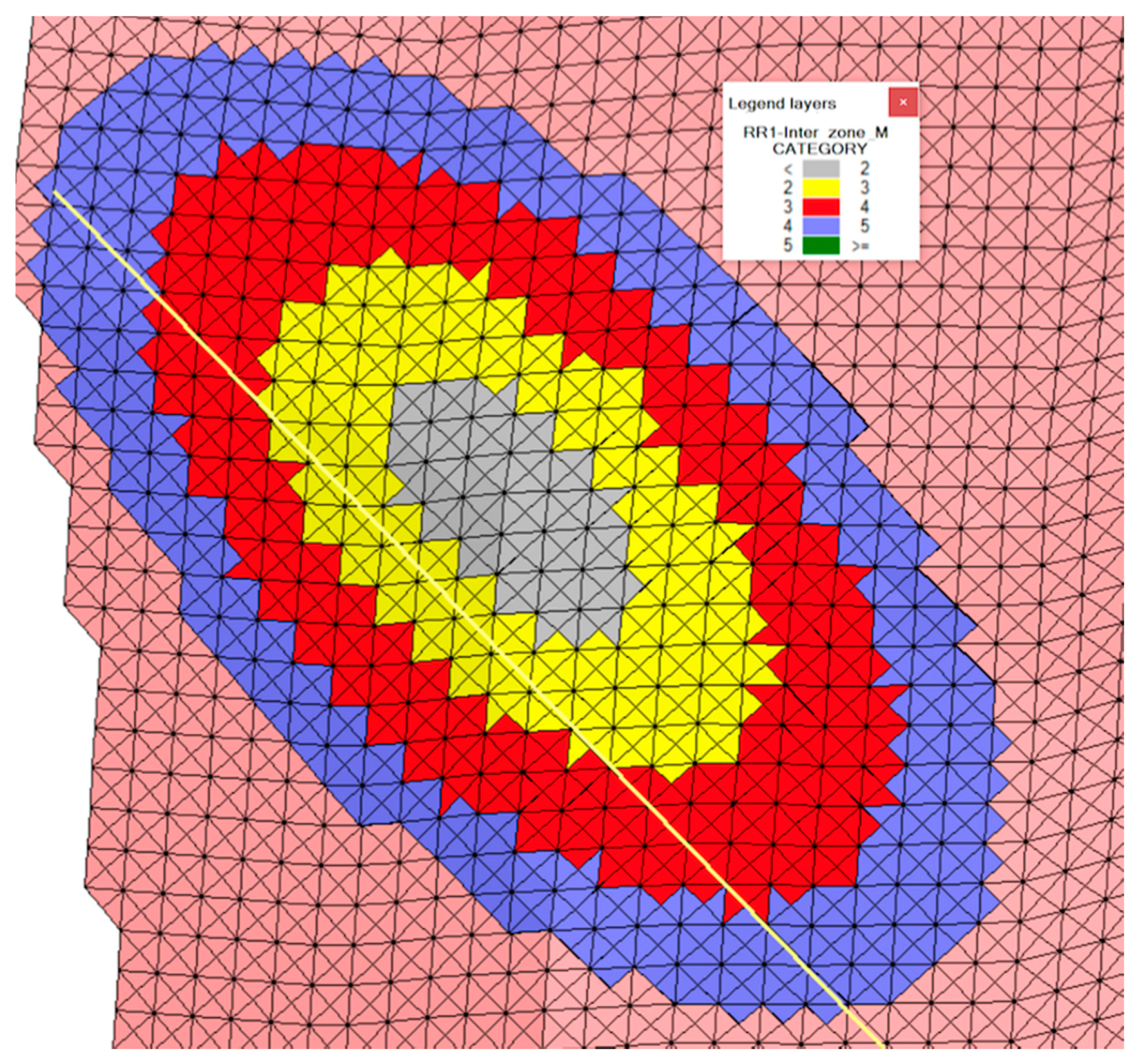
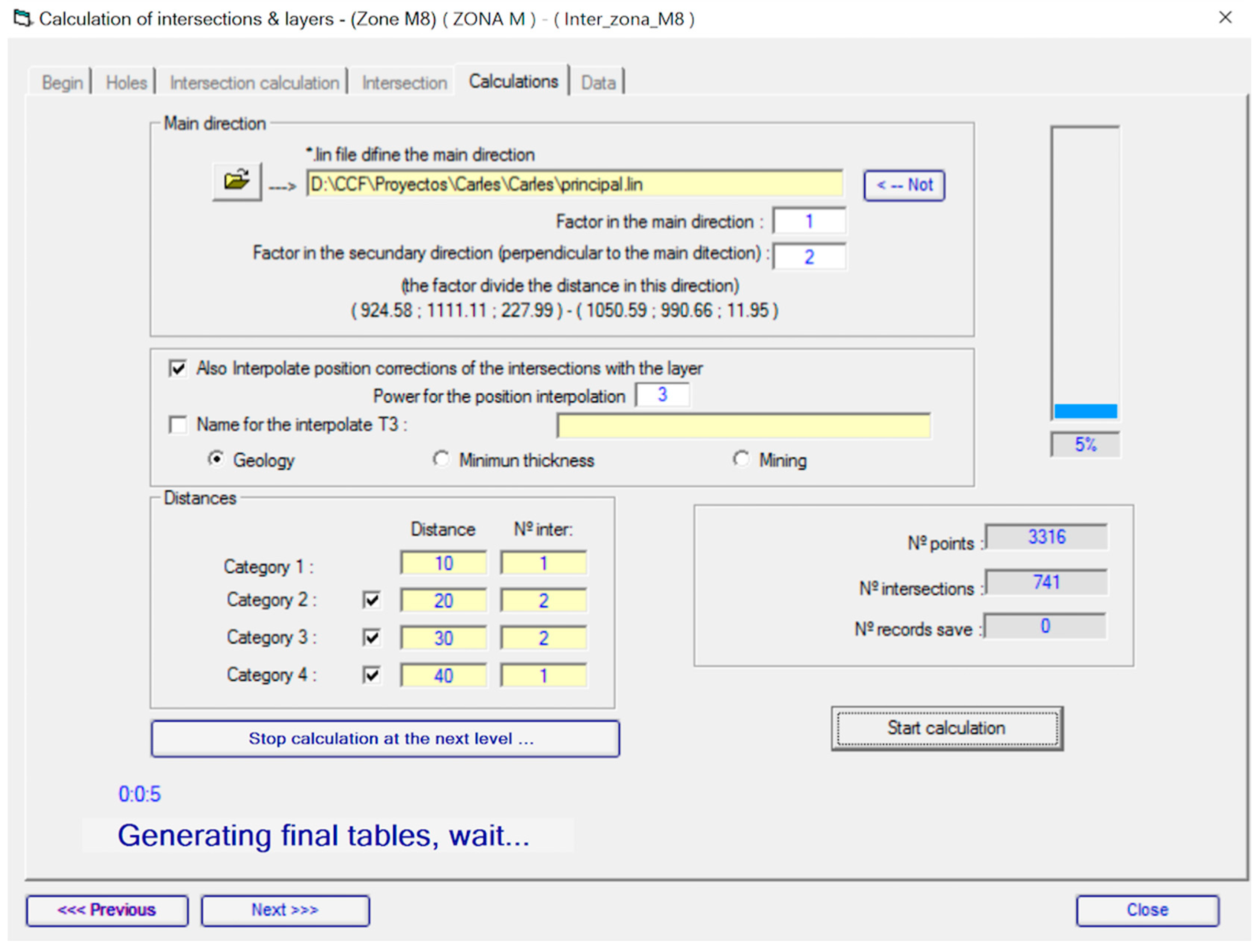
4.8. Definition of the Estimation Categories and Generation of the Calculation Units

As in any other resource estimation method, the interpolation level of confidence must be defined. This is done through the use of the so-called categories. The algorithm uses up to four categories (measured, indicated, inferred or proven, and probable). The position of samples in the octant can be used if necessary, avoiding and/or adjusting calculations according to the number of samples present in opposite octants surrounding the calculation point. In the example shown here, four numerical categories are used:

• Category 1: calculation units with an intercept at less than 10 m
• Category 2: calculation units with two intercepts at less than 20 m
• Category 3: calculation units with two intercepts at less than 30 m
• Category 4: calculation units with one intercept at less than 40 m

In these category calculations, the distance reduction defined by the main and secondary axis of the ellipsoid is also taken into account.

4.9. Calculation Units Generation and Categories Definition

Some parts of the calculation method are based on the generation of provisional data sheets created through the addition of data queries. This method allows fast operations across the entire data set.

The SQL language was also used to make the selections and differentiate, quickly and with low coding effort, between the different calculation types.

The generated information was stored in a relational database (BDT2), from where it is retrieved by the drawing module. Figure 15 shows the last tab of the calculation window, where the total amounts corresponding to a certain cutoff grade can be seen, as well as the total for each category.

The influence by percentage of each borehole of the total amount of weight and interpolated elements can also be obtained (

Table 3. Influence percentage by borehole.

D.Hole	Tons	Au_e	Cu	Au	Ag
CN1014	1.5%	1.90%	0%	2%	1%
CN1015	2.9%	14.90%	9.7%	15.4%	16.6%
CN1016	1.9%	2.00%	1.2%	2.1%	1.5%
CN1017	0.4%	1.40%	0.8%	1.5%	1.2%
CN1018	0.2%	1.30%	0.9%	1.3%	0.8%
CN1019	0.6%	0.40%	0.5%	0.4%	1.0%
CN1020	1.1%	0.60%	0.7%	0.6%	0.9%
CN1021	0.7%	0.90%	1.0%	0.9%	1.4%
CN1022	0.6%	0.10%	0.0%	0.1%	0.2%
CN1023	1.5%	1.50%	1.6%	1.4%	2.1%
CN1024	1.2%	0.70%	0.0%	0.8%	0.0%
CN1025	0.6%	0.50%	0.6%	0.5%	0.9%
CN1026	0.6%	0.50%	0.7%	0.4%	0.9%
CN1027	0.9%	0.60%	1.1%	0.6%	0.8%
CN1028	0.9%	0.50%	0.6%	0.5%	0.4%
CN1029	0.6%	0.70%	0.0%	0.8%	0.0%
CN1030	0.7%	0.10%	0.0%	0.1%	0.1%
CN1031	0.7%	0.20%	0.0%	0.2%	0.0%
CN1032	0.7%	0.60%	0.8%	0.6%	0.5%

). This allows for the checking of the results, specifically searching for balanced results and avoiding overweighed boreholes. The main results can be guided by a very low number of boreholes, which can result in a significant variation if sample mistakes are present. Figure 16 shows SQL guided results analysis, which allows for powerful, quick, and easy selection of data. Figure 17A shows the 3D results of the SQL selection and the associated legend colors. Please notice that the seam width variation is adequately simulated, as shown in Figure 17B.

5. Method Suitability

This method has been called the “Pentahedral Method” due to the fact that the calculation unit has a shape close to a pentahedron: two triangular faces connected by three four-sided faces. Nevertheless, it is clear that it is not a pentahedron, but rather an octahedron, as the faces with four sides could have their vertices on different planes; that is, each of them is made up of two triangular faces (Figure 11A).

This method is a calculation alternative in the case of these seam-shaped mineral structures, as it can work in three dimensions and be completely computer-programmable.

It is suited to seams with extremely pronounced folds, as seen in Figure 18.

Compared to classic block models the pentahedral method offers several advantages, such as:

• Any change in the calculation parameters does not need the calculation units to be redefined.
• When defining the calculation geometry units, these can be separately prepared for subsequent exploitation and scheduling, even exporting them to other software.
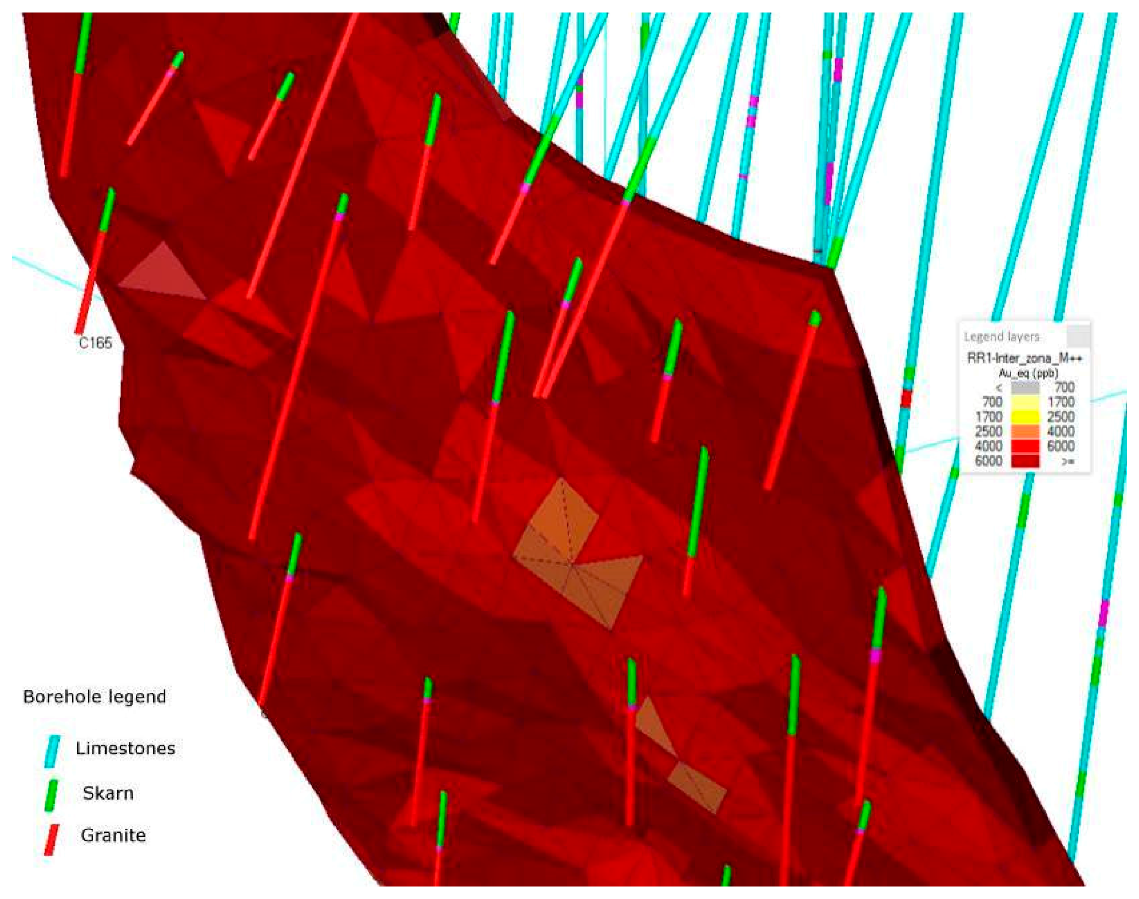
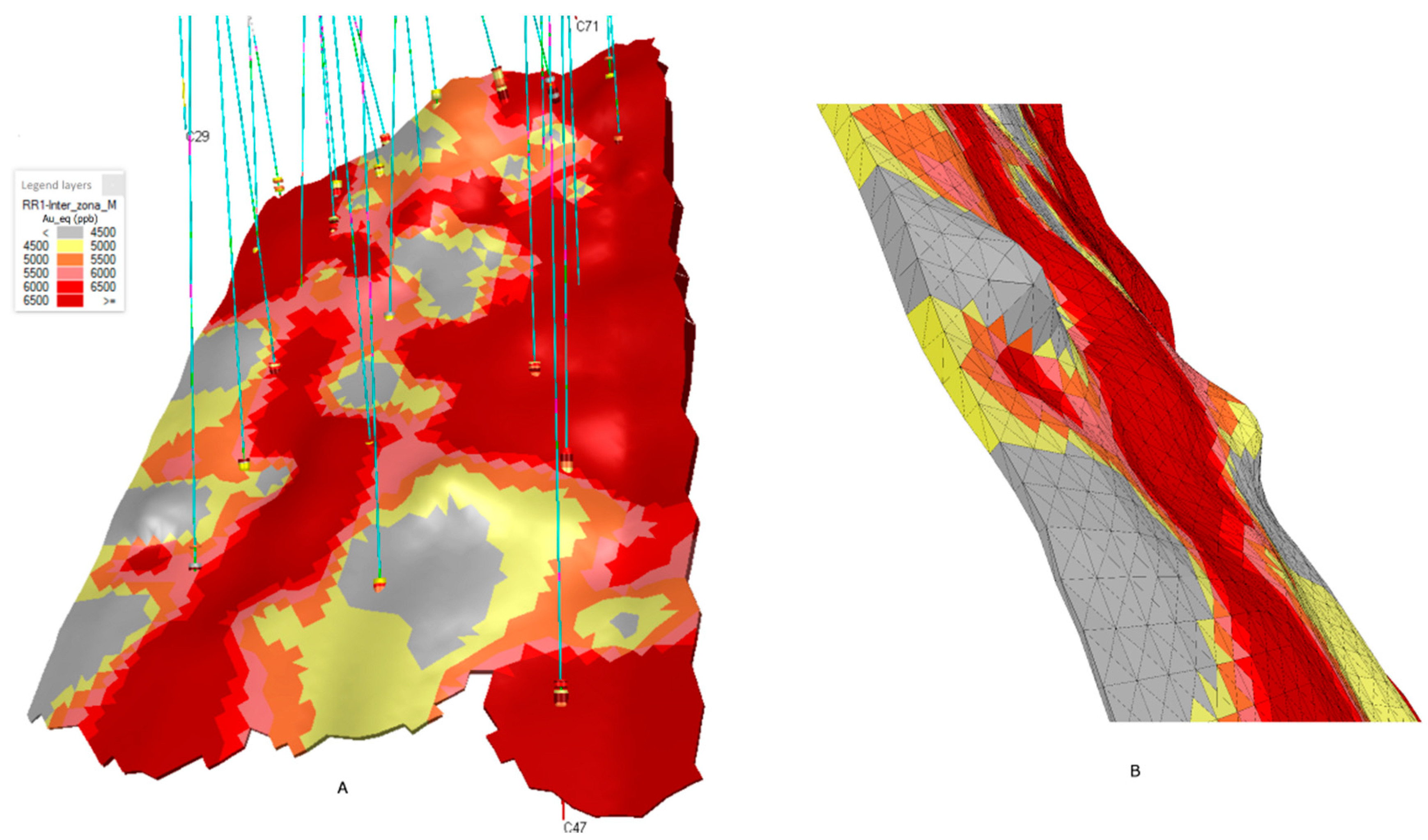
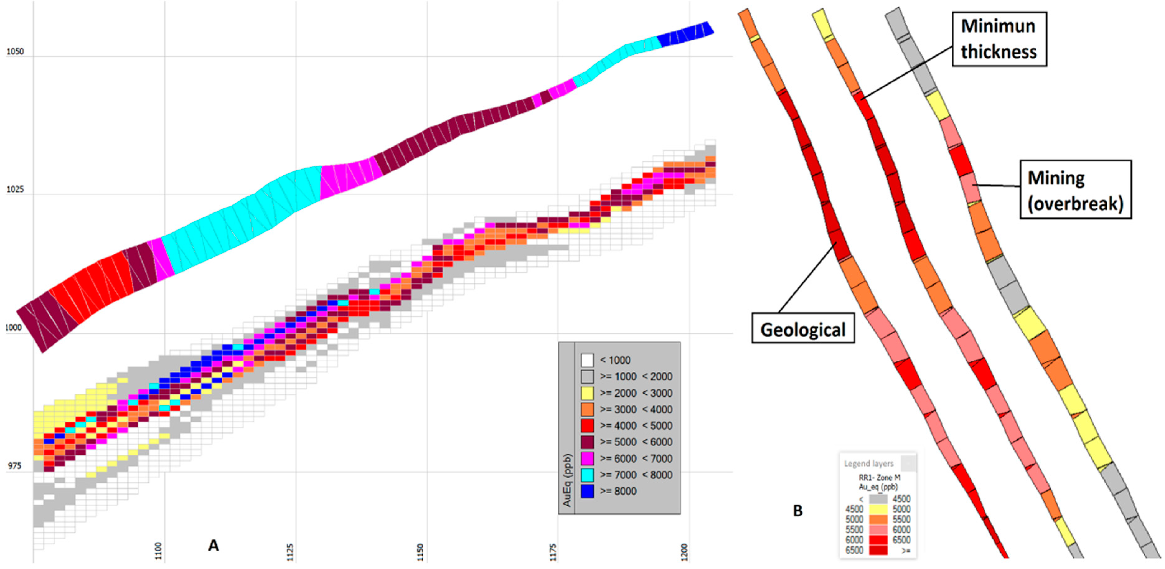
• It provides a fairly accurate representation of the thickness of the seam-shaped structure even in the case of low thickness seams, which is extremely difficult to achieve with traditional block models (Figure 19).
• It interpolates intersections, not samples taken from boreholes.
• Geometrical results closely follow the deposit limits, as opposed to block models that create a stair-shaped profile (see Figure 19).
• It includes the possible internal dilution, as well as the lateral dilution due to mining overbreak.
• A minimum thickness can be defined according to mining technical conditions.

This method could be also used to model larger ore deposits or even regional scale geological seams, such as the ones shown in [21].

6. Discussion and Conclusions

This paper shows that, in the case of mineral ore bodies that are seam-shaped, using the new “Pentahedral Method” it is possible to obtain an evaluation of the reserves and resources with a higher degree of accuracy than with the classic block method.

Compared to other methods such as the polygon method, the triangle method, or the section one, this methodology is more advanced, allowing interpolation with the intercepts. This method can be applied to all types of seams, even those with extremely pronounced folds, and it allows work to be conducted in 3D and to be a good representation of the ore body to be obtained. Figure 20 is a U3D model that can be embedded in the pdf of the paper, which shows interactively what has been explained throughout this paper.

This method also offers several additional advantages compared to the classic block model concept, mainly in its three-dimensional representation capabilities. Regarding interpolation, it also allows any method to be used, even kriging, as well as the use of search ellipsoids.

The use of SQL databases to store the results allows reports and results analysis to be issued very quickly.

The introduction of calculation variables such as “overbreak” “dilution” or “minimum thickness” gives more information from the resources data to the technician in charge of the reserves definition. These variables are related to the mining process and will simplify the reserve calculation as it will eliminate some of the resources that are not economically exploitable.

These results can be used for mine planning and design where final reserves will be defined, and have already been included in some versions of the Recmin software. At this stage the method has not been prepared to be used with other software, although it could be adapted to generate data and share it through simple ASCII files where block data are coded.

The method has passed the preliminary exam of the international patent PCT/ES03/00117, achieving positive results; the research is recognized as innovative, it implies research activity and it can be applied in the industry.

References

1. Wang, G.; Zhang, S.; Yan, C.; Song, Y.; Li, D. Mineral potential targeting and resource assessment based on 3D geological modelling in Luanchuan region, China. Comput. Geosci. 2011, 37, 1976–1988. [Google Scholar] [CrossRef]
2. Canadian Institute of Mining. CIM Definition Standards on Mineral Resources and Mineral Reserves; CIM Definition Standards (2014); Canadian Institute of Mining, Metallurgy and Petroleum: Quebec, QC, Canada, 2014. [Google Scholar]
3. Annels, A.E. Mineral Deposit Evaluation: A Practical Approach; Chapman & Hall: London, UK, 1991. [Google Scholar]
4. Clark, I. Practical Geostatistics; Applied Science Publishers Ltd.: London, UK, 1979. [Google Scholar]
5. Clark, I.; Harper, W.V. Practical Geostatistics 2000; Ecosse North America Llc.: Columbus, OH, USA, 2001; 342p. [Google Scholar]
6. Rendu, J.M. An Introduction to Geostatistical Methods of Mineral Evaluation; South African Institute of Mining and Metallurgy: Johannesburg, South Africa, 1981. [Google Scholar]
7. Castañón, C. Nuevo Método de Cálculo de Recursos Geológicos y Reservas Mineras para Yacimientos Tabulares y Aplicación Informática para la Gestión Integral de un Proyecto Minero. Ph.D. Thesis, Universidad de Oviedo, Asturias, Spain, 2006; 200p. [Google Scholar]
8. Silva, D.S.F.; Boisvert, J.B. Mineral resource classification: A comparison of new and existing techniques. J. S. Afr. Inst. Min. Metall. 2014, 114, 265–273. [Google Scholar]
9. Will Gemcom Produce a Leaped Frog out of Leapfrog? Available online: http://www.orefind.com/blog/orefind_blog/2012/11/14/will-gemcom-produce-a-leaped-frog-out-of-leapfrog- (accessed on 10 February 2017).
10. Rossi, M.E.; Deutsch, C.V. Mineral Resource Estimation; Springer: London, UK, 2014; p. 332. [Google Scholar]
11. Boisvert, J.B.; Deutsch, C.V. Programs for kriging and sequential Gaussian simulation with locally varying anisotropy using non-Euclidean distances. Comput. Geosci. 2011, 37, 495–510. [Google Scholar] [CrossRef]
12. Martín-Izard, A.; Fuertes, M.; Cepedal, A.; Maldonado, C.; Pevida, L.R.; Spiering, E.; González, S.; Varela, A. Geochemical characteristisc of the Río Narcea gold belt intrusives and timing of development of the different magmatic-hydrothermal processes based on K/Ar dating. In Gold Exploration and Mining in NW Spain; Arias, D., Martín-Izard, A., Paniagua, A., Eds.; University of Oviedo: Asturias, Spain, 1998; pp. 35–42. [Google Scholar]
13. Martín-Izard, A.; Fuertes-Fuente, M.; Cepedal, A.; Moreiras, D.; García-Nieto, J.; Maldonado, C.; Pevida, L.R. The Río Narcea Gold Belt intrusions: Geology, petrology, geochemistry and timing. J. Geochem. Explor. 2000, 71, 103–117. [Google Scholar] [CrossRef]
14. Spiering, E.D.; Pevida, L.R.; Maldonado, C.; González, S.; García, J.; Varela, A.; Arias, D.; Martín-Izard, A. The gold belts of western Asturias and Galicia (NW Spain). J. Geochem. Explor. 2000, 71, 89–101. [Google Scholar] [CrossRef]
15. Pevida, L.R.; Maldonado, C.; Spiering, E.; González, S.; García, J.; Varela, A.; Martín-Izard, A.; Cepedal, A.; Fuertes, M. Geology and exploration guides along the Río Narcea gold belt. In Gold Exploration and Mining in NW Spain D; Arias, D., Martín-Izard, A., Paniagua, A., Eds.; University of Oviedo: Asturias, Spain, 1998; pp. 27–36. [Google Scholar]
16. Martın-Izard, A.; Paniagua, A.; García-Iglesias, J.; Fuertes-Fuente, M.; Boixet, L.L.; Maldonado, C.; Varela, A. The Carlés copper-gold-molybdenum skarn (Asturias, Spain): Geometry, mineral associations and metasomatic evolution. J. Geochem. Explor. 2000, 71, 153–175. [Google Scholar] [CrossRef]
17. Castañón, C. Manual de Ayuda del Software Minero RecMin. 2006. Available online: http://recmin.com/WP/?page_id=255 (accessed on 8 May 2017).
18. Meinert, L.D. Skarns and skarn deposits. In Ore Deposit Models; Sheahan, P.A., Cherry, M.E., Eds.; Geological Association of Canada: St. John’s, NL, Canada, 1993; Volume II, pp. 117–134. [Google Scholar]
19. Bustillo, M.; López-Jimeno, C. Manual de Evaluación y Diseño de Explotaciones Mineras; Entorno Gráfico S.L.: Madrid, Spain, 1997. [Google Scholar]
20. The Stanford Geostatistical Modeling Software (SGeMS). Available online: http://sgems.sourceforge.net/ (accessed on 10 February 2017).
21. Galera, C.; Bennis, C.; Moretti, I.; Mallet, J.L. Construction of coherent 3D geological blocks. Comput. Geosci. 2003, 29, 971–984. [Google Scholar] [CrossRef]
Figure 1. (A) Geological map of the Carlés gold-bearing skarn (data provided by Rio Narcea Gold Mines); (B) Section of the Carlés deposit (West Carlés); (C) Section of the Carlés deposit (North Carlés).
Minerals 07 00072 g001
Figure 2. (A) View of the stratigraphic control of the skarn development at the Carlés skarn. The monzogranite intrusion is also controlled by the sedimentary layers; (B) Close-up view of stratigraphically controlled Carlés mineralized banded skarn. Bands are dominated by pyroxene-magnetite alternate with garnet-amphibole-rich bands.
Minerals 07 00072 g002
Figure 3. Example of a mineralized area in an intercepting borehole.
Minerals 07 00072 g003
Figure 4. T1 surface generation. (A) A cross section of boreholes is depicted in white and the intercepts with the body are depicted in red. The green line connects the centers of each red line section; (B) Sections and their corresponding centerlines, which are triangulated to generate a surface. (C) Calculated surface (“T1”).
Minerals 07 00072 g004
Figure 5. Example of base surface T1 (left (A)) converted to calculation Surface T2 (right (B)). Detail of meshing points in sections and in crossing diagonals of any generated square (C).
Minerals 07 00072 g005
Figure 6. Intercept calculation of four boreholes (S1 to S4) through a seam-shaped mineral ore body. A (geology intercept), B (minimum thickness intercept), C (mining overbreak intercept); U, V, and W are points of the NPS; i1–i4 are the lithology intercept interval; d1–d4 distances between the intercepts center and W point.
Minerals 07 00072 g006
Figure 7. RecMin Iinput window for intercept parameters. Holes selection (all, in this case), cutoff, minimum thickness, overbreak (one side), and maximum waste thickness.
Minerals 07 00072 g007
Figure 8. RecMin Output window, intercept graph bars for C1163 borehole: red (geological intercept), yellow (minimum thickness intercept), and white (mining overbreak intercept).
Minerals 07 00072 g008
Figure 9. Table of calculated intercepts calculated in RecMin. Results for several boreholes. First column is the name of the borehole (down hole). Each hole has three data rows showing the intercept data.
Minerals 07 00072 g009
Figure 10. Definition of the guide line of the interpolation ellipse drawn over T2. A theoretical borehole crosses the seam and defines several possible categories of resources, according to the distance between the NPS points and the location of intersection center point.
Minerals 07 00072 g010
Figure 11. Calculation unit as used in the pentahedral method (A). Volume calculation (B) and calculation graphic exploded (C).
Minerals 07 00072 g011
Figure 12. Mineral seam filled with calculation units, as automatically obtained by the software. Boreholes are colored by lithology. The legend refers to grade over seam (ppb).
Minerals 07 00072 g012
Figure 13. Calculation parameters in the interpolation of the pentahedral method.
Minerals 07 00072 g013
Figure 14. Example of economical seam center (blue line) vs. theoretical seam center (green line).
Minerals 07 00072 g014
Figure 15. Numerical results of the “Pentahedral Method,” classified by intercept type and category.
Minerals 07 00072 g015
Figure 16. Assistant module used to open the pentahedral files and obtain a 3D visualization, as per SQL database conditions restrictions.
Minerals 07 00072 g016
Figure 17. 3D view, pentahedral filled seam representing orebody “Zona M” of the Carlés deposit (A). Detail of the variable width of the calculated seam (B). The legend shows the Au grade, expressed in ppb.
Minerals 07 00072 g017
Figure 18. Extremely pronounced fold in mineral seam.
Minerals 07 00072 g018
Figure 19. Graphic comparison between the block model (conventional method) and the “Pentahedral Method”. Left (A): plane section of the blocks that define the seam colored according to grade and the same calculated seam; Right (B): sections of the three different types of calculation done in the same seam.
Minerals 07 00072 g019
Figure 20. 3D model of the calculated seam colored by grade, including in the user selectable layers the topography and boreholes colored according to geology and sample grading.
Minerals 07 00072 g020