Spatial Mapping of the Rock Quality Designation Using Multi-Gaussian Kriging Method


Department of Mining Engineering, School of Mining and Geosciences, Nazarbayev University, Astana 010000, Kazakhstan
*
Author to whom correspondence should be addressed.
Minerals 2018, 8(11), 530; https://0-doi-org.brum.beds.ac.uk/10.3390/min8110530
Submission received: 22 August 2018
/
Revised: 18 October 2018
/
Accepted: 25 October 2018
/
Published: 15 November 2018
Abstract
:The rock quality designation is an important input for the analysis and design of rock structures as reliable spatial modeling of the rock quality designation (RQD) can assist in designing and planning mines more efficiently. The aim of this paper is to model the spatial distribution of the RQD using the multi-Gaussian kriging approach as an alternative to the non-linear geostatistical technique which has shown some limitations. To this end, 470 RQD datasets were collected from 9 boreholes pertaining to the Gazestan ore deposit in Iran. The datasets were declustered then transformed into Gaussian distribution. To ensure the model spatial continuity, variogram analysis was first performed. The elevation 150 m with a grid of 5 m × 5 m × 5 m was selected to illustrate the methodology. Surface maps showing the RQD classes (very poor, poor, fair, good, and very good) with their associated probability were established. A cross-validation method was used to check the obtained model. The validation results indicated good prediction of the local variability. In addition, the associated uncertainty was quantified on the basis of the conditional distributions and the accuracy plot agreed with the overall results. It is concluded that the proposed model could be used to produce a reliable RQD map.
1. Introduction
Zoning of subsurface materials based on 3D modeling of quantitative description of rock mass quality is a powerful tool in different disciplines of civil and mining engineering paradigm. The geomechanical parameters logged from boreholes are explicitly able to provide sufficient information for the quality of rocks and their dominated region. Because of the importance of these geomechanical variables, extensive research works have been carried out from the correct way of its determination to its spatial representation [1,2,3]. Recent applications of spatial rock quality designation (RQD) characterization in the geosciences include mine slope design [4], geomechanical properties of rock mass [5], geohazard zonation mapping [6], tunneling [7], probabilistic evaluation of RQD [8], geometallurgical studies [9]. In general, spatial prediction of regionalized variables by linear geostatistical methodology such as kriging is a common practice. However, a smoothing effect in the kriged results imposes difficulty in interpretation of the estimated map, it shows, for which a notable variance reduction in the conditional cumulative distribution. This also is associated with over- and under-estimation of low and high values, respectively [10], when one is comparing the interpolated map with original variability of the underlying dataset. Beside this reasonable criticism, some geomechanical parameters like RQD are non-additive and cannot be modeled by these types of linear interpolation methodologies [11]. Non-additivity of a variable implies that its mean value does not correspond to the arithmetic average and consequently, 3D mapping of such a variable is challenging. However, in this context, there are some applications of different paradigm aspect of kriging for spatial visualization of RQD such as ordinary kriging [7,12,13] and indirect estimation integrating the secondary variable by indicator kriging [8]. Non-linear geostatistical modeling such as geostatistical simulation as an alternative is strongly recommended for the spatial characterization of geomechanical variables since there is no requirement for linear averaging [14,15,16]. For instance, the RQD can be conditionally simulated by sequential simulation [17] and turning band simulation [18]. In particular, Madani and Asghari [19] employed sequential Gaussian simulation to define probabilistically the faulted areas. Although simulation approaches turn the joint uncertainty into an efficient avenue, computational time and post-processing for managing the realizations are notable [20]. Other non-linear geostatistical functions can also be considered including lognormal kriging, disjunctive kriging, and indicator kriging [21]. Nevertheless, those approached are suffering from smoothing effect for skewed distribution and it has been showed that the estimation results are relatively poor in this latter case [22]. Multi-Gaussian kriging as another non-linear geostatistical technique has been widely accepted among practitioners due to no smoothing effect. In this concept, two groups of multi-Gaussian kriging called simple and ordinary were proposed for recoverable resource assessments and mapping the probabilities in mineral resource evaluation and delineation of geochemical anomalies in exploration of mineral deposits [23]. The simple multi-Gaussian kriging assumes that the mean value is perfectly known through the region and then restricts its usage only to stationary domains [24]. To overcome this impediment, Emery [24] introduced an approach to substitute the unknown mean for random variable constant through the region and, advantageously, the true conditional distribution could be met [24]. This method is highly recommended in the case of some domains, including the trend in the variability of attributes under study, where universal kriging is problematic in variogram analysis [25,26].
Despite of the benefits of the multi-Gaussian kriging, this methodology is developed successfully only for uncertainty quantification above a certain threshold [24]. This means uncertainty between two consecutive thresholds cannot be calculated in a reliable way. The aim of this study is fourfold: (1) presentation of the Multi-Gaussian methodology and updating the current algorithm, which would allow computing of the uncertainty between the consecutive thresholds; (2) employing the methodology to model the spatial distribution of RQD in a phosphate ore deposit located in Iran; (3) post-process, the estimation of results to obtain the probabilistic maps of the desirable rock quality intervals, examine the RQD variability along the elevation and detect the possible faulted areas; and (4) model validation and conclusion.
2. Materials and Methods
2.1. Multi-Gaussian Kriging
Multi-Gaussian kriging is a non-linear geostatistical methodology, for which the mean and variance of the estimated maps follow the multivariate normality assumption, while they are obtained from the conventional kriging system [10]. This fundamental theory entails the anterior distribution of the variable under study to be Gaussian normal standard with mean and variance equal to 0 and 1, respectively. Simple multi-Gaussian kriging is applicable when the random field is Gaussian and show stationary characteristics on its first and second order moments (mean and variance). The formula is defined as [27]:
where, is Simple multi-Gaussian kriging, is Simple kriging estimation, is Simple kriging variance, is a standard Gaussian random vector independent of the conditional data. With respect to the stationary assumption i.e., constant mean, the applicability of simple multi-Gaussian kriging is somewhat restrictive and not really agreeable. This crucial drawback manifests itself where particularization of the mean is misinterpreted. In contrast, ordinary multi-Gaussian kriging for the sake of overcoming this condition is becoming more actionable. Emery [28] proposed the fundamental theory of ordinary multi-Gaussian kriging to make the estimator more wide spread-used and robust to the non-stationary variability in the domain by replacing the unknown mean by random variable constant over the space. The ordinary multi-Gaussian kriging can be defined as the follow:
where, is Ordinary multi-Gaussian kriging, is Ordinary kriging estimation, is Ordinary kriging variance, is a standard Gaussian random vector independent of the conditional data. In this study, the ordinary multi-Gaussian kriging is applied to quantification of uncertainty in RQD measure (subsequent section). So, in order to perform the experiment through multi-Gaussian kriging, the below general instruction should be followed: exploratory data analysis, declustering, normal score transformation of the raw variable, variogram analysis over the Gaussian values, estimation of the Gaussian variables (simple or ordinary), back transformation to the original variable and uncertainty quantification and cross-validation, (Figure 1).
2.1.1. Quantification of Uncertainty Function
An interesting utilization of multi-Gaussian kriging is quantification of uncertainty at un-sampled locations. To do so, uncertainty functions or recovery functions in mining application, allow one to assess the uncertainty of the variable under study above a given threshold or between two thresholds via expected value of its conditional distribution [24,28]:
In practice, the expectation can be computed by Monte Carlo integration [24,28,29]:
where N is a large positive integer and are realizations of drawn by Latin hypercube sampling which is a kind of stratified sampling method.
Therefore, the actual uncertainty function between two given thresholds and can be calculated by the following function [24,28]:
where, I(.) is an indicator function, equal to 1 if estimated value is between and , 0 otherwise. By this Formula (5), the probability of finding the estimated value between two consecutive thresholds can straightforwardly be calculated. One application in this study is characterized to map the probability of finding the estimated RQD between two thresholds that give the related rock mass quality at un-sampled locations. In following sections, this idea is practically presented and discussed thoroughly over a case study located in Iran.
3. Case Study: Gazestan Ore Deposit in Iran
Gazestan ore deposit is located close to Bafg province in Central Iran (Figure 2). Rock settings belong to Rizu formation and consist of carbonate sediments, shale, sandstone, volcanic rocks. Intrusive rocks are stock and dike including gabbros diorite, gabbros, and diabase with some outcrop within the area as well as sedimentary and volcanic rocks. Green rocks with acidic components have phosphate and iron-ore mineralization, which in some parts show depth facies. Alteration in volcanic rocks is more obvious and consists of silication, feldespatization, chloritization, and forming of mafic minerals such as epidote, tremolite, and actinolite. Apatite mineralization occurs as apatite and magnetite lens, veins and nodules, in strongly chloritized pyroxenes mafic diabase. The value of P2O5 varies between 3% and 38%, and values of rare earth elements (REEs) in apatite mineral exceed 1.5%. Detailed exploratory studies show that tens of millions of tons of ores with 10–15% mean grade of P2O5 and tents (REEs) are predictable in this ore deposit [30]. Based on the structural viewpoint, Gazestan ore deposit belongs to the central Iran zone and Poshtebadam-Bafq. Faulting and fracturing system in the area have been divided into three groups and one thrusting [19,30].
Using the case phosphate ore deposit of Gazestan in Iran, the spatial distribution of RQD through ore deposits is purposed to model via the ordinary multi-Gaussian kriging algorithm. RQD introduced by Deere et al. [31] as a long-lived classification system and also as one of the input variables of the two well-known rock classification systems, RMR and Q systems. The RQD which is initially proposed as a measure of the quality of borehole core is defined as the ratio in percentage of the total length of sound core pieces that is 10 cm or longer to the length of the core run. On the basis of the RQD values, the rock mass could be classified in terms of its quality as very poor, poor, fair, good, and very good for an RQD values <25%, 25–50%, 51–75%, 76–90% and 91–100%, respectively. Detail RQD measurement is performed on 9 boreholes having depth from 49 to 173 m and the data points ranging from 23 to 86 along the holes. The boreholes including BH8, BH12, BH15, BH6, and BH7 are vertical and rest of them is inclined as given detail in Table 1 and Figure 3.
3.1. Exploratory Data Analysis
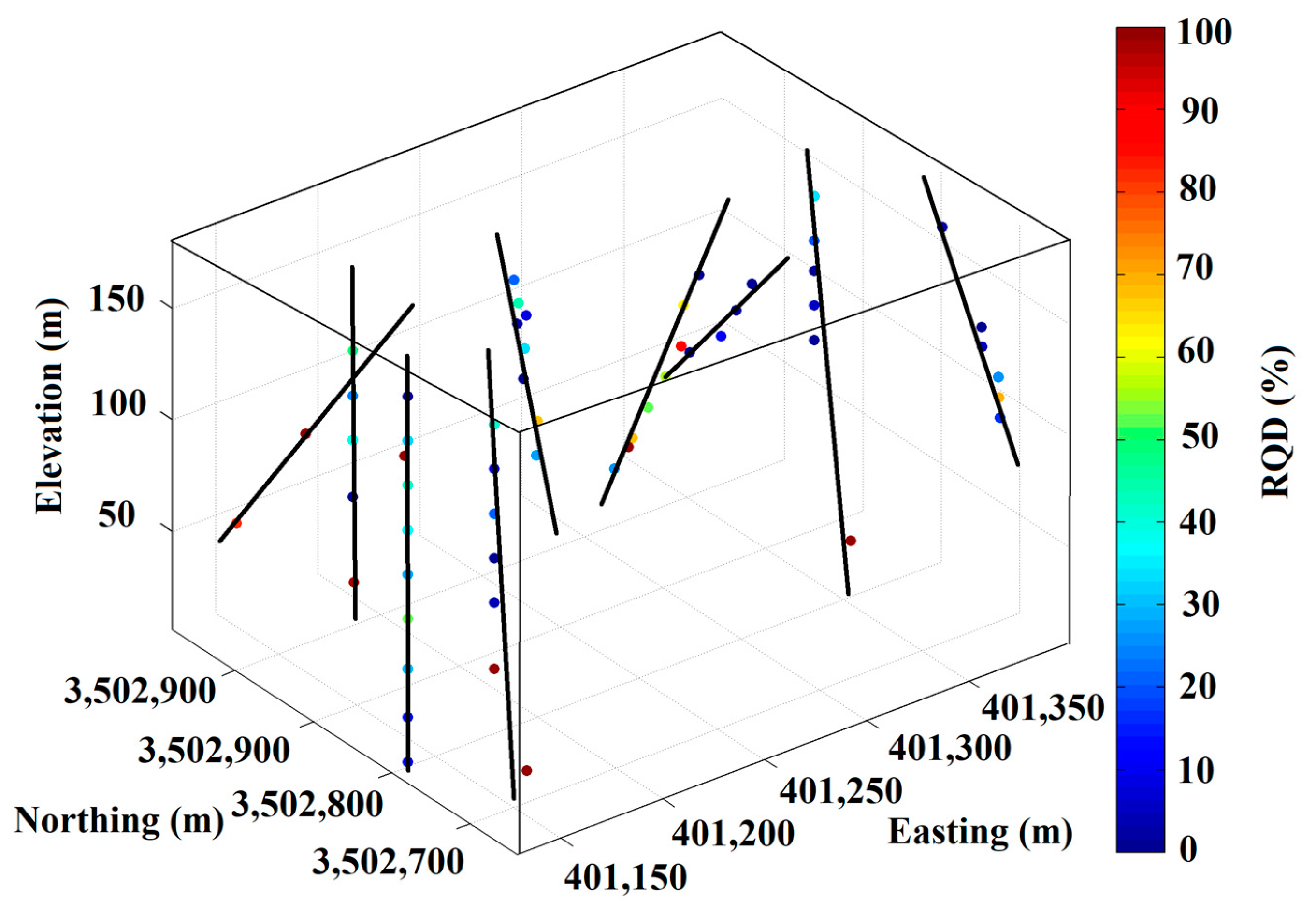
In the Gazestan Ore deposit area where the original data for a total of 470 samples belong to 9 boreholes are examined to perform this study. Position, coordinates and location of boreholes in the study area are given as 3D in Figure 4. As discussed previously, some boreholes are inclined and some of them are vertical and depth of boreholes are various as well as data obtained from each hole. The range of RQD varies from about 6 to 100% as discussed previously. It is obvious that the rock mass is quite jointed and the quality of the rock various from very poor to fair rocks. As the aim of this work is to show the capability of the methodology to quantify uncertainty, some synthetic boreholes are added to the middle region. To do so, first some random locations are generated and distributed; then by turning band simulation [28], the RQD variables are simulated on those locations conditionally to the data available in the boreholes. This ensures that the simulated values has the same statistical characteristics as the borehole data and enhance the visualization of RQD variability in the region wherein the samples are examined in an exploratory way.
In order to perform multi-Gaussian kriging, the conditional samples should then be transformed to Gaussian normal distribution (step 1). The drilling patterns are commonly irregular and it needs a declustering technique [32] to provide a representative distribution of the variable of interest in the region. Through this technique, the weights are allocated to each location considering the closeness to the surrounding RQD data. A summary of descriptive statistics of the RQD samples for both original and synthetic boreholes that vary continuously between 0% and 100%, respectively. The resulting average value for RQD is 39.21%, with a standard deviation of 33.34 and a sample variance of 1111.5. The cumulative distribution functions of RQD variable in the field is given in Figure 5. In this graph, the abscissa shows the RQD values ordered from smallest to largest and the ordinate represents the cumulative probability assigned to each data [33]. The different domains of rock mass quality are identified in this curve and one compute the proportion of each separately. Accordingly, the proportions for the underlying rock qualities of very poor, poor, fair, good, and excellent are 43.86%, 20.53%, 16.32%, 6.67%, and 12.63%, respectively (Figure 5).
3.2. Transformation to Gaussian Distribtuion
Step 2 in the multi-Gaussian kriging procedure is to transfer the declustered data to normal standard distribution . The reason why the data should be Gaussian distributed is that the prediction of uncertainty at un-sampled locations are based on conditioning the normal standard data [10]. Therefore, a Gaussian anamorphosis function is used to transform the RQD data into a Gaussian variable with mean 0 and variance 1. In this approach, one constructs the sample cumulative histogram by applying declustering weights. This methodology entails that the transformed variable of RQD has a Gaussian distribution with mean and variance equal to 0 and 1, respectively (Figure 6).
After transformation, it is of interest to check whether the transformed variable follows the bivariate normality since multi-Gaussian kriging assumption is based on the bivariate normality. This can be implemented by checking the experimental variogram of different order (w) through the transferred Gaussian values (proper explanation of variogram is presented in Section 3.5). This paradigm is based on the comparison between the usual variogram and the variogram of lower order. The latter corresponds to madogram and rodogram, for which the power in variogram formula is 1 and 1/2, respectively. In order to show that the bigaussian assumption between two variables is respected, Emery [34] verified that plotting the experimental variogram with those different orders against the conventional experimental variogram in log–log coordinates should be almost aligned the theoretical lines. This theory is employed over the normal score RQD variable in this study and as can be seen in Figure 7, the points are distributed along the thick solid lines with a reasonable deviation. This graph implies that the normal values are somehow in acceptable agreement with bi-Gaussian characteristics and one can apply the multi-Gaussian kriging over the underlying dataset.
3.3. Modeling Spatial Continuity: Variogram Analysis
Spatial continuity of geological properties including geomechanical parameters can be a measure of changes in variance versus distance. To do so, experimental variogram computes the average dissimilarity between data separated by vector . It is calculated as half the average squared difference between the components of every data pair [10,35]:
where is an h-increment of the variable and is the number of pairs.
As explained above, the modogram and rodogram can also be defined as (Deutsch and Journel, 1998):
Modogram:
Rodogram:
Two applications can be identified for these two latter functions with smaller power. The first one corresponds to analysis of bigaussianity characteristics as explained above. Since modogram and rodogram are not influenced by extreme values, another application is based on the detection of anisotropy and approximate ranges of the variable under study in the region [36]. The anisotropy shows that how much continuity exists among the pairs of samples. Maximum and minimum spatial continuity is a requirement for every geostatistical methodology and should be defined prior to any variogram analysis. Therefore, in this study, modogram and rodogram are computed over the declustered RQD values in three directions (azimuth: 0, 45, 90) with lag of 20 m in the plan and in one direction with lag of 12 m perpendicular to the plan including 50% of tolerance in both lag and azimuth (Figure 8). The comparable dashed lines in the plan corroborates that the maximum and minimum ranges of anisotropy are identical in the plan. However, red dashed line toward the vertical direction shows a small deviation relevant to the one obtained from plan. Those results turn out the idea of one isotropy characteristic in the plan and one perpendicular anisotropy toward the vertical.
After coming up with the decision to perform anisotropy of RQD in the region, variogram analysis is performed on the transformed RQD data to model the related spatial structure. One omnidirectional variogram and one vertical directional variogram is calculated and fitted with two Spherical models (Figure 9), using two basic nested structures:
The plotted models show that the related variogram has geometric anisotropy.
3.4. Multi-Gaussian Kriging Results
Multi-Gaussian kriging is performed on a regular grid with dimension of 5 m × 5 m× 5 m for prediction of RQD. In this algorithm, the ordinary kriging is used since it is independent of the mean and its stationary behavior [28]. A moving neighborhood is constructed based on the variogram ranges and set to 200 and 150 for horizontal and vertical dimensions, respectively containing up to 50 original data points the surrounding area. The RQD like just other geomechanical parameters is non-additive [32]. It means that the average of these kind of measurements do not follow the linear averaging [16]. As a result, for applying the kriging or any other estimation methodologies, one cannot discretize the block and point support should be considered. In this research, the RQD values are estimated in the center of the block and no discretization is treated in the process of modeling. Figure 10 shows a plan view of the estimated RQD in the elevation of 80 m after back transformation to the original distribution as a general consideration. This plan (Figure 10) is selected since it demonstrates an interesting variability of the high quality of rocks in the middle of the region.
3.5. Probabilistic Description for Each Rock Mass Quality Domain
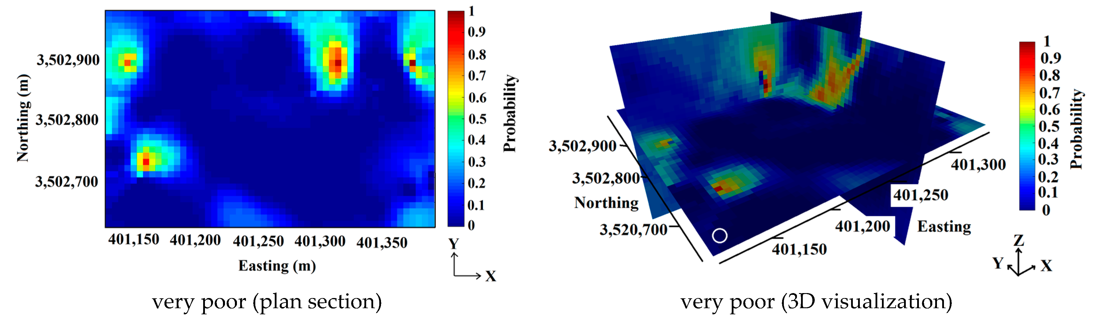
As discussed above in Section 2.1.1, the uncertainty function can be calculated by Equation (5). The idea of this section is to quantify the local uncertainty (probability) of the underlying domains which specify the rock mass quality of that region according to the data obtained from boreholes. These maps are constructed by computing, for each block, the frequency of occurrence of each rock quality domain over 500 realizations drawn from Equation (4) (Figure 11). They present the risk of finding a domain different from others. The sectors with little uncertainty are those affiliated with a high probability for a given rock quality domain (colored in red in Figure 11), shows that there is a little risk of nor finding this rock quality domain, or those affiliated with a very low probability (colored in dark blue in Figure 11), indicating that one pretty sure of not finding this domain, while the other sectors (colored in light blue, green, or yellow in Figure 11) are more uncertain. In the following subsections, two applications of those probabilistic maps are presented as an example to interpret the sub-surface characterization of rock domains. They can then be incorporated into the further analysis for mine and tunnel design.
3.5.1. Application of Probabilistic Maps
Vertical Variability of RQD
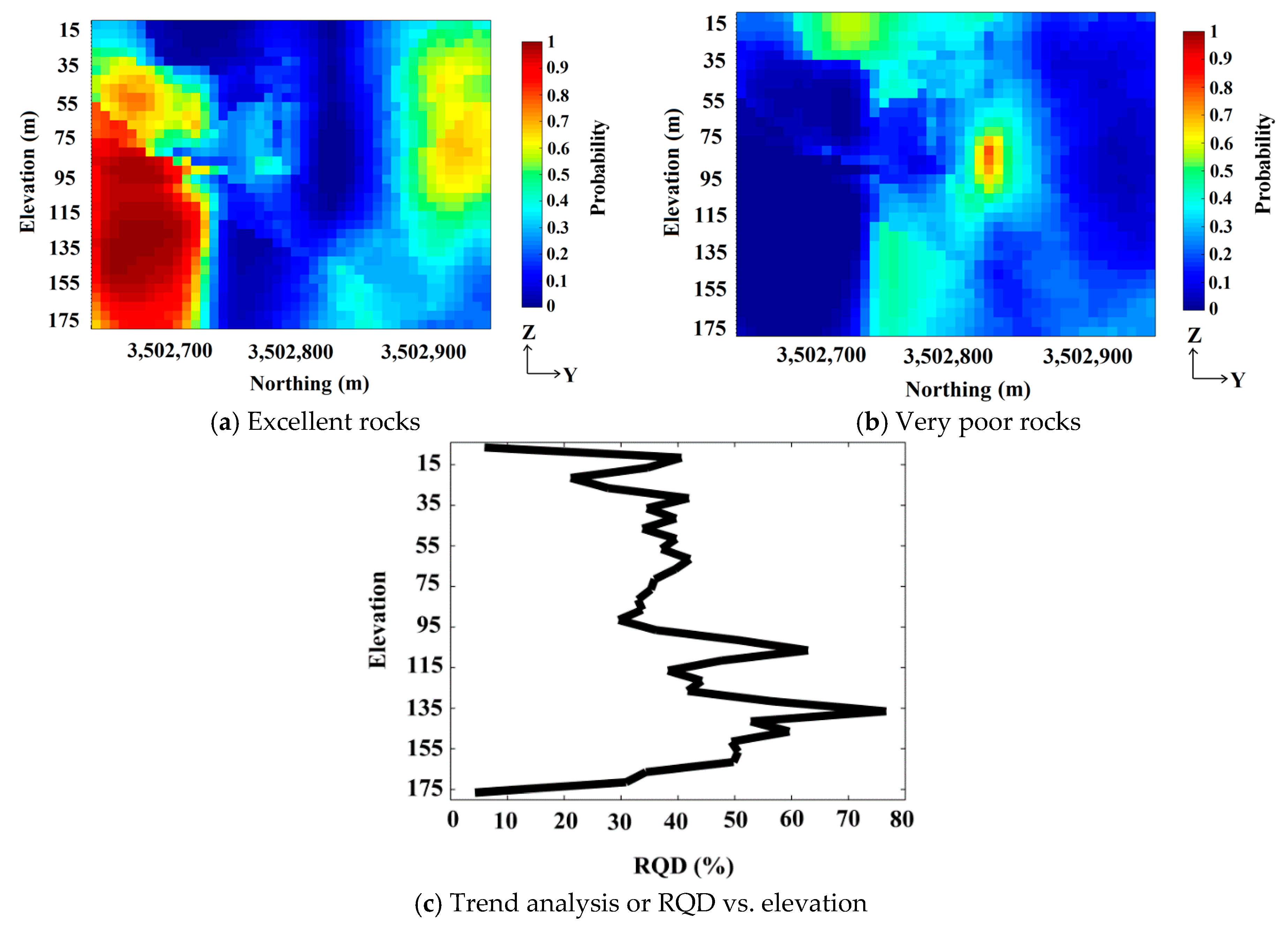
In this subsection, it is of interest to show how the multi-Gaussian results can be incorporated into the analysis of rock quality variability along the depth. As a matter of fact, it is highly probable to find the excellent rocks at a great depth rather that close to surface. This is corroborated with relative density. However, since the geological phenomena are full of complexities, this concept might be tedious to verify in whole occasions. In this study, the trend analysis over the variability of RQD is also examined alongside the elevation. This graph is helpful to quickly scan fluctuations of the variable under study in order to define possible inherent trends in the region. Figure 12c shows that the rocks close to the surface are poorly structured and by increasing the depth, the quality of rock increases steadily up to elevation 135 m. Beyond this elevation, one can see that the tendency of RQD is toward a decline. This characteristic is dramatically recognized in the produced maps of multi-Gaussian kriging, in which this trend is highly correlated with the statistics of the borehole dataset (Figure 12a,b). It is worth mentioning that the trend analysis over the borehole dataset, is the average of all the samples in each elevation and consequently, it is slightly over and underestimated due to the mixture of the high and low values. In this case, the tendency of the variable is sound enough to interpret the recognition of possible trends in the region under study. For instance, in a particular case, at elevation 135 m, it stems from trend analysis that the quality of rocks in this area is such a high value, in which finding the good quality of rocks are highly probable. In contrast, around elevation 0 to 75 m, the poor qualities of rocks are extremely predictable. These two are also confirmed by the result of multi-Gaussian kriging maps at vertical section of 401,144 m.
Detection of Possible Faulted Boundaries
Another interesting results that can be considered in the output of multi-Gaussian kriging, is to detect the possible areas for fault systems. In this study, following Madani and Asghari [19], the faulted region can be recognized by producing the probabilistic outputs of excellent rocks. The difference here is that this map is generated by multi-Gaussian kriging, for which the modeling time is more reasonable than geostatistical simulation approach. As can be seen from Figure 13, those possible areas are nominated according to the visual location of hard and soft rocks. For the sake of simplicity, in this figure, we can say that the red areas show the excellent rocks while the blue areas illustrate the rocks of poor quality. The spatial location of these two regions implies the faulted region.
3.6. Model Validation
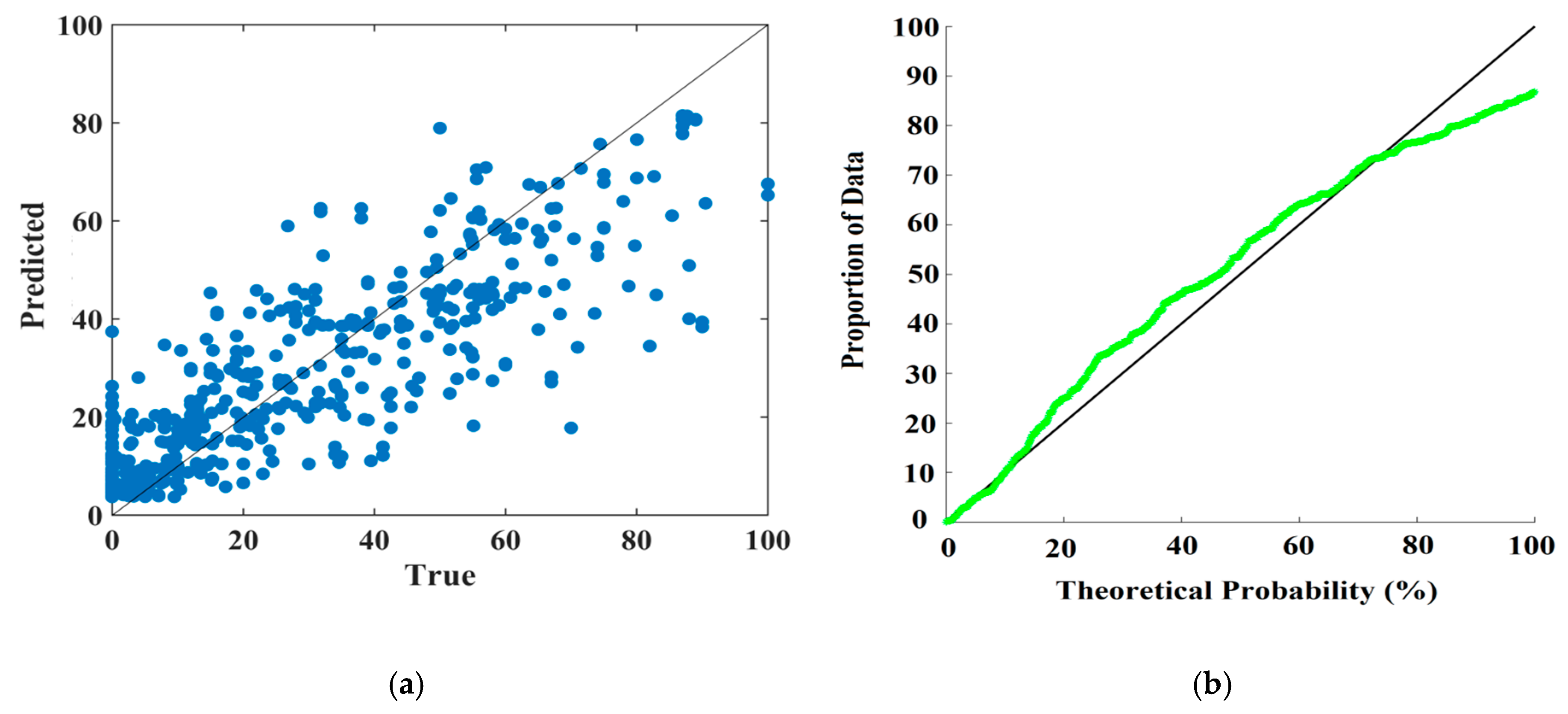
In order to validate the predictions and constructed model obtained by ordinary multi-Gaussian kriging, at each data location, the cross-validation procedure has been performed. The rationale of this method is that actual data are removed one at a time and re-estimated based upon the remaining data situated in the estimation neighborhood. Each data attribute is replaced when it has been re-estimated [32]. Once the true and estimated values for each location are accessible, the mean relative error and correlation coefficient as a measure of accuracy can be quantified. A scatter diagram between the true and predicted RQD is given in Figure 14a. According to this validation, the correlation coefficient between the predicted and true RQD is 87.58 and mean relative error, as another measure of prediction accuracy for this technique is 0.301, in which this small value implies that the spatial estimation of data location by cross-validation gives reasonable results and one can trust to the probabilistic description of RQD variability at un-sampled locations. The uncertainty model can also be validated thorough the conditional distributions using the probability intervals varies from 0.1 to 0.9 [24]. Those values can then be plotted against the fractions of data that actually belong to the intervals so defined (Figure 14b). As can be seen, the plot illustrates an acceptable match and therefore, a correct modeling of the local uncertainty is observed.
4. Results and Discussion
We presented an update version of the current Multi-Gaussian kriging algorithm, making possible to compute the uncertainty block-by-block in the region. This spatial modeling is fast and efficient in terms of time computation, comparing with other type of non-linear geostatistical approaches such as stochastic simulation. The difference between this technique and the methodology applied by Madani and Asghari [19] for uncertainty quantification of RQD attribute is explained in this section. Madani and Asghari [19] employed a sequential Gaussian simulation algorithm to model the RQD variable, in which it allows the uncertainty quantification in fault boundaries. Although the simulation algorithm is straightforward and easy to use, it has some drawbacks. First, computation time is demanding for post processing the simulation results (realizations) in order to define the probabilistic characterization of a regionalized variable [37]. Next, Gaussian simulation needs a full random function and not just a variogram model [10]. Last, although the sequential Gaussian simulation technique is simple and tractable in alternative fields of data variation [38], the accuracy of this method is not always guaranteed [39,40,41,42] and care must be taken to design of the neighborhood structure, particularly in the case of non-stationary phenomena (i.e., heterogeneous variability). By contrast, the multi-Gaussian kriging algorithm that is proposed in this study has, relatively, some advantageous. It is remarkably efficient in terms of computation time and is capable of directly producing the uncertainty measures (e.g., probability maps and conditional variance) while establishing the multi-Gaussian kriging system. Furthermore, since the ordinary multi-Gaussian kriging is no longer dependent on the local variations of the mean value in the domain of interest, and the non-stationary variables (e.g., heterogeneous RQD) can be modeled by this approach. Compared to other non-linear geostatistical algorithms, such as indicator kriging, multi-Gaussian kriging does not suffer from order-relation problems, due to the mathematical consistency of its conditional distribution; indicating that further correction procedures are not required. Further extensions of this method proposed in this work can also be generalized to multivariate situations, in the case when the RQD values have quite satisfying spatial and global correlation with other geomechanical co-variates (such as RMR, GSI, and Q) in the domain. Here, one can deal with joint uncertainty quantification, respecting the cross-correlation among the variables, obtaining by substitution of the co-kriging [43] for kriging in multi-Gaussian kriging system.
5. Conclusions
In this paper, a multi-Gaussian kriging approach for simulating the spatial distribution of the RQD was presented to overcome some limitations of the non-linear geostatistical technique. A 3D surface map of RQD was established allowing a spatial visualization of the RQD classes (very poor, poor, fair, good, and very good) with their associated probability. The usefulness of these RQD maps was discussed. The cross-validated results showed a correlation coefficient between the predicted and actual RQD was R = 87.58 while the mean relative error 0.301 indicating good accuracy. In addition, the associated uncertainty was validated on the basis of the conditional distributions and the obtained probability matched the overall results. These results were in agreement with those of some related works recently published.
The current work highlighted several advantages. Theoretical results and the case study demonstrated that this methodology was able to calculate in a reliable manner the joint uncertainty at un-sampled locations. The results of this study can serve as basis for future developments on the mapping of geo-metallurgical variables such as RMR, GSI, Q, ore grades, etc. It is concluded that, the current methodology can assist to spatially model the RQD which is important for mining designs and for downstream mining engineering paradigm optimization. However, this method can be developed to adjust the desired proportion in each category which enhance improves the quality of outputs.
Author Contributions
N.M., S.Y. and A.C.A. conceived, designed the experiments and wrote the paper.
Funding
The first author acknowledges the Nazarbayev University for funding this work via ‘‘Faculty development competitive research Grants for 2018–2020’’ under Contract No. 090118FD5336.
Acknowledgments
The first author acknowledges the Geological Survey & Mineral Exploration of Iran (GSI) for providing the Gazestan dataset.
Conflicts of Interest
The authors declare no conflict of interest. The founding sponsors had no role in the design of the study; in the collection, analyses, or interpretation of data; in the writing of the manuscript, and in the decision to publish the results.
References
- Parra, A.; Morales, N.; Vallejos, J.; Vuong Nguyen, P.M. Open pit mine planning considering geomechanical fundamentals. Int. J. Min. Reclam. Environ. 2017, 32, 221–238. [Google Scholar] [CrossRef]
- Singh, V.K.; Prasad, M.; Singh, S.K.; Rao, D.G.; Singh, U.K. Slope design based on geotechnical study and numerical modelling of a deep open pit mine in India. Int. J. Surf. Min. Reclam. Environ. 2007, 9, 105–111. [Google Scholar] [CrossRef]
- Santos, V.; da Silva, P.F.; Brito, M.G. Estimating RMR Values for Underground Excavations in a Rock Mass. Minerals 2018, 8, 78. [Google Scholar] [CrossRef]
- Khakestar, M.S.; Hassani, H.; Moarefvand, P.; Madani, H. Prediction of the collapsing risk of mining slopes based on geostatistical interpretation of geotechnical parameters. J. Geol. Soc. India 2016, 87, 97–104. [Google Scholar] [CrossRef]
- Eivazy, H.; Esmaieli, K.; Jean, R. Modelling Geomechanical Heterogeneity of Rock Masses Using Direct and Indirect Geostatistical Conditional Simulation Methods. Rock Mech. Rock Eng. 2017, 50, 3175–3195. [Google Scholar] [CrossRef]
- Masoud, A.A.; Aal, A.K.A. Three-dimensional geotechnical modeling of the soils in Riyadh city. KSA Bull. Eng. Geol. Environ. 2017, 1–17. [Google Scholar] [CrossRef]
- Ozturk, C.A.; Simdi, E. Geostatistical investigation of geotechnical and constructional properties in Kadikoy–Kartal subway. Turk. Tunn. Undergr. Sp. Technol. 2014, 41, 35–45. [Google Scholar] [CrossRef]
- Oh, S. Geostatistical integration of seismic velocity and resistivity data for probabilistic evaluation of rock quality. Environ. Earth Sci. 2013, 69, 939–945. [Google Scholar] [CrossRef]
- Burger, B.; McCaffery, K.; McGaffin, I.; Jankovic, A.; Valery, W.; La Rosa, D. Batu Hijau model for throughput forecast, mining and milling optimization, and expansion studies. In Advances in Comminution; Kawatra, K., Ed.; SME: Englewood, CHI, USA, 2006; p. 461. [Google Scholar]
- Chilès, J.-P.; Delfiner, P. Geostatistics: Modeling Spatial Uncertainty. Wiley Series in Probability and Statistics; John Wiley & Sons, Inc.: Hoboken, NJ, USA, 2012. [Google Scholar] [CrossRef]
- Coward, S.; Vann, J.; Dunham, S.; Stewart, M. The primary-response framework for geometallurgical variables. In Proceedings of the Seventh International Mining Geology Conference, Perth, Australia, 17–19 August 2009. [Google Scholar]
- Liu, Y.P.; He, S.H.; Wang, D.H.; Li, D.Y. RQD prediction method of engineering rock mass based on spatial interpolation. Yantu Lixue/Rock Soil Mech. 2015, 36, 3329–3336. [Google Scholar]
- Ryu, J.-S.; Kim, M.-S.; Cha, K.-J.; Lee, T.H.; Choi, D.-H. Kriging interpolation methods in geostatistics and DACE model. KSME Int. J. 2002, 16, 619–632. [Google Scholar] [CrossRef]
- Boisvert, J.B.; Rossi, M.E.; Ehrig, K.; Deutsch, C.V. Geometallurgical Modeling at Olympic Dam Mine. South Aust. Math. Geosci. 2013, 45, 901–925. [Google Scholar] [CrossRef]
- Newton, M.J.; Graham, J.M. Spatial Modelling and Optimisation of Geometallurgical Indices. In Proceedings of the Second AusIMM International Geometallurgy Conference (GeoMet), Brisbane, Australia, 30 September–2 October 2011; pp. 247–261. [Google Scholar]
- Deutsch, C.V. Geostatistical modelling of geometallurgical variables—Problems and solutions. In Proceedings of the Second AusIMM International Geometallurgy Conference (GeoMet), Brisbane, Australia, 30 September–2 October 2013; pp. 7–16. [Google Scholar]
- Assari, A.; Mohammadi, Z. Analysis of rock quality designation (RQD) and Lugeon values in a karstic formation using the sequential indicator simulation approach, Karun IV Dam site. Iran Bull. Eng. Geol. Environ. 2017, 76, 771–782. [Google Scholar] [CrossRef]
- Ellefmo, S.L.; Eidsvik, J. Local and Spatial Joint Frequency Uncertainty and its Application to Rock Mass Characterisation. Rock Mech. Rock Eng. 2008, 42, 667. [Google Scholar] [CrossRef]
- Madani Esfahani, N.; Asghari, O. Fault detection in 3D by sequential Gaussian simulation of Rock Quality Designation (RQD). Arab. J. Geosci. 2013, 6, 3737–3747. [Google Scholar] [CrossRef]
- Deutsch, J.L.; Palmer, K.; Deutsch, C.V.; Szymanski, J.; Etsell, T.H. Spatial Modeling of Geometallurgical Properties: Techniques and a Case Study. Nat. Resour. Res. 2016, 25, 161–181. [Google Scholar] [CrossRef]
- Hekmatnejad, A.; Emery, X.; Alipour-Shahsavari, M. Comparing linear and non-linear kriging for grade prediction and ore/waste classification in mineral deposits. Int. J. Min. Reclam. Environ. 2017. [Google Scholar] [CrossRef]
- Moyeed, R.A.; Papritz, A. An Empirical Comparison of Kriging Methods for Nonlinear Spatial Point Prediction. Math. Geol. 2002, 34, 365–386. [Google Scholar] [CrossRef]
- Afzal, P.; Madani, N.; Shahbeik, S.; Yasrebi, A.B. Multi-Gaussian kriging: A practice to enhance delineation of mineralized zones by Concentration–Volume fractal model in Dardevey iron ore deposit. SE Iran J. Geochem. Explor. 2015, 158, 10–21. [Google Scholar] [CrossRef]
- Emery, X. Uncertainty modeling and spatial prediction by multi-Gaussian kriging: Accounting for an unknown mean value. Comput. Geosci. 2008, 34, 1431–1442. [Google Scholar] [CrossRef]
- Armstrong, M. Problems with universal kriging. J. Int. Assoc. Math. Geol. 1984, 16, 101–108. [Google Scholar] [CrossRef]
- Cressie, N. A nonparametric view of generalized covariances for kriging. Math. Geol. 1987, 19, 425–449. [Google Scholar] [CrossRef]
- Rivoirard, J. Introduction to Disjunctive Kriging and Nonlinear Geostatistics; Oxford University Press: Oxford, UK, 1994. [Google Scholar]
- Emery, X. Two Ordinary Kriging Approaches to Predicting Block Grade Distributions. Math. Geol. 2006, 38, 801–819. [Google Scholar] [CrossRef]
- Marechal, A. Recovery Estimation: A Review of Models and Methods. In Geostatistics for Natural Resources Characterization: Part 1; Verly, G., David, M., Journel, A.G., Marechal, A., Eds.; Springer: Dordrecht, The Netherlands, 1984; pp. 385–420. [Google Scholar]
- Jamali, S. Gazestan Ore Deposit Exploration; Geological Survey of Iran: Tehran, Iran, 2008. [Google Scholar]
- Deere, D.U.; Hendron, A.J.; Patton, F.D.; Cording, E.J. Design of Surface and Near-Surface Construction in Rock. In Proceedings of the 8th U.S. Symposium on Rock Mechanics (USRMS), Minneapolis, MN, USA, 15–17 September 1966. [Google Scholar]
- Deutsch, C.V.; Journel, A. GSLIB: Geostatistical Software and User’s Guide, 2nd ed.; Oxford University Press: New York, NY, USA, 1998. [Google Scholar]
- Davis, J.C. Statistics and Data Analysis in Geology; Wiley: New York, NY, USA, 1986. [Google Scholar]
- Emery, X. Variograms of Order ω: A Tool to Validate a Bivariate Distribution Model. Math. Geol. 2005, 37, 163–181. [Google Scholar] [CrossRef]
- Maleki, M.; Emery, X.; Mery, N. Indicator Variograms as an Aid for Geological Interpretation and Modeling of Ore Deposits. Minerals 2017, 7, 241. [Google Scholar] [CrossRef]
- Goovaerts, P. Geostatistics for Natural Resources Evaluation; Oxford University Press: New York, NY, USA, 1997. [Google Scholar]
- Rossi, M.E.; Deutsch, C.V. Mineral Resource Estimation; Springer: Berlin, Germany, 2014. [Google Scholar]
- Alabert, F.G.; Massonnat, G.J. Heterogeneity in a complex turbiditic reservoir: Stochastic modelling of facies and petrophysical variability. In Proceedings of the 65th Annual Technical Conference and Exhibition of the Society of Petroleum Engineers, SPE-20604, London, UK, 30–31 October 1990; pp. 775–790. [Google Scholar]
- Emery, X. Testing the correctness of the sequential algorithm for simulating Gaussian random fields. Stoch. Environ. Res. Risk Assess. 2004, 18, 401–413. [Google Scholar] [CrossRef]
- Emery, X.; Peláez, M. Assessing the accuracy of sequential Gaussian simulation and cosimulation. Comput. Geosci. 2011, 15, 673–689. [Google Scholar] [CrossRef]
- Paravarzar, S.; Emery, X.; Madani, N. Comparing sequential Gaussian and turning bands algorithms for cosimulating grades in multi-element deposits. C. R. Geosci. 2015, 347, 84–93. [Google Scholar] [CrossRef]
- Eze, P.N.; Madani, N.; Adoko, A.C. Multivariate Mapping of Heavy Metals Spatial Contamination in a Cu–Ni Exploration Field (Botswana) Using Turning Bands Co-simulation Algorithm. Nat. Resour. Res. 2018. [Google Scholar] [CrossRef]
- Madani, N.; Emery, X. A comparison of search strategies to design the cokriging neighborhood for predicting coregionalized variables. Stoch. Environ. Res. Risk Assess. 2018. [Google Scholar] [CrossRef]
Figure 1.
Schematic instruction for multi-Gaussian kriging. (NSCORE data: normal score transformation data).
Figure 1.
Schematic instruction for multi-Gaussian kriging. (NSCORE data: normal score transformation data).

Figure 2.
Geological map and location of 9 boreholes and the study area.

Figure 3.
Average distribution of rock quality designation (RQD) for each borehole in the field.

Figure 4.
3D location map 9 boreholes drilled in the study area; complexity in the ore deposit imposed inclined boreholes to capture the potential phosphorus in the area.
Figure 4.
3D location map 9 boreholes drilled in the study area; complexity in the ore deposit imposed inclined boreholes to capture the potential phosphorus in the area.

Figure 5.
Cumulative distribution probability plot; the red dashed lines show the different categories according to the rock mass quality.
Figure 5.
Cumulative distribution probability plot; the red dashed lines show the different categories according to the rock mass quality.

Figure 6.
Global distribution of RQD variable (histogram) before and after transformation.

Figure 7.
Experimental madograms and rodogram of the Gaussian variables as a function of their experimental variograms.
Figure 7.
Experimental madograms and rodogram of the Gaussian variables as a function of their experimental variograms.

Figure 8.
Modogram and rodogram for detection of anisotropy for RQD variable; red line shows the vertical anisotropy.
Figure 8.
Modogram and rodogram for detection of anisotropy for RQD variable; red line shows the vertical anisotropy.

Figure 9.
Direct variograms of Gaussian variables (cross points: experimental variogram and solid lines: theoretical variogram modeled to the experimental).
Figure 9.
Direct variograms of Gaussian variables (cross points: experimental variogram and solid lines: theoretical variogram modeled to the experimental).

Figure 10.
Multi-Gaussian kriging of RQD, high quality rocks are distributed in the middle of the region.
Figure 10.
Multi-Gaussian kriging of RQD, high quality rocks are distributed in the middle of the region.

Figure 11.
Probability maps for different rock mass qualities at elevation 80 m.


Figure 12.
Probability maps produced from multi-Gaussian kriging for two different rock qualities in vertical section (Easting: 401,411 m).
Figure 12.
Probability maps produced from multi-Gaussian kriging for two different rock qualities in vertical section (Easting: 401,411 m).

Figure 13.
Possible detection of faulted region in the study area (section; Easting: 401299).

Figure 14.
Validation of results. (a) Cross-validation for prediction vs. true values; black line: diagonal line (R = 87.58, MSE = 0.30); (b) Probabilities versus fractions of data that belong to probability intervals; solid line: identity; green line: accuracy plot.
Figure 14.
Validation of results. (a) Cross-validation for prediction vs. true values; black line: diagonal line (R = 87.58, MSE = 0.30); (b) Probabilities versus fractions of data that belong to probability intervals; solid line: identity; green line: accuracy plot.


Table 1.
Statistical description of RQD for each borehole.
| Boreholes | Max | Average | Min | Stdev | Length of Boreholes (m) | Number of Data Points | Type of Boreholes |
|---|---|---|---|---|---|---|---|
| BH8 | 100.00 | 58.31 | 0.00 | 25.54 | 125.07 | 70 | Inclined |
| BH11 | 83.00 | 32.15 | 0.00 | 17.37 | 173.5 | 86 | Vertical |
| BH12 | 71.00 | 32.26 | 3.00 | 22.84 | 49.6 | 23 | Inclined |
| BH14 | 66.00 | 40.13 | 0.00 | 16.17 | 95.0 | 35 | Vertical |
| BH15 | 88.00 | 33.92 | 0.00 | 26.83 | 118.41 | 59 | Inclined |
| BH5 | 55.12 | 16.02 | 0.00 | 14.69 | 103.8 | 53 | Vertical |
| BH6 | 41.30 | 12.21 | 0.00 | 12.43 | 79.75 | 50 | Inclined |
| BH7 | 78.80 | 23.13 | 0.00 | 22.86 | 75.36 | 47 | Inclined |
| BH10 | 22.30 | 5.57 | 0.00 | 6.10 | 75.24 | 47 | Vertical |
© 2018 by the authors. Licensee MDPI, Basel, Switzerland. This article is an open access article distributed under the terms and conditions of the Creative Commons Attribution (CC BY) license (http://creativecommons.org/licenses/by/4.0/).
Share and Cite
MDPI and ACS Style
Madani, N.; Yagiz, S.; Coffi Adoko, A. Spatial Mapping of the Rock Quality Designation Using Multi-Gaussian Kriging Method. Minerals 2018, 8, 530. https://0-doi-org.brum.beds.ac.uk/10.3390/min8110530
AMA Style
Madani N, Yagiz S, Coffi Adoko A. Spatial Mapping of the Rock Quality Designation Using Multi-Gaussian Kriging Method. Minerals. 2018; 8(11):530. https://0-doi-org.brum.beds.ac.uk/10.3390/min8110530
Chicago/Turabian StyleMadani, Nasser, Saffet Yagiz, and Amoussou Coffi Adoko. 2018. "Spatial Mapping of the Rock Quality Designation Using Multi-Gaussian Kriging Method" Minerals 8, no. 11: 530. https://0-doi-org.brum.beds.ac.uk/10.3390/min8110530
Note that from the first issue of 2016, this journal uses article numbers instead of page numbers. See further details here.