Health Assessment of Complex System Based on Evidential Reasoning Rule with Transformation Matrix

Abstract

In current research of complex system health assessment with evidential reasoning (ER) rule, the relationship between the indicators reference grades and pre-defined assessment result grades is regarded as a one to one correspondence. However, in engineering practice, this strict mapping relationship is difficult to meet, and it may degrease the accuracy of the assessment. Therefore, a new ER rule-based health assessment model for a complex system with a transformation matrix is adopted. First, on the basis of the rule-based transformation technique, expert knowledge is embedded on the transformation matrix to solve the inconsistent problems between the input and the output, which keeps completeness and consistency of information transformation. Second, a complete health assessment model is established via the calculation and optimization of the model parameters. Finally, the effectiveness of the proposed model can be validated in contrast with other methods.

1. Introduction

A complex system, for instance, control system [1], servo system [2], energy storage system [3], is widely used in aviation, aerospace, electronics and other fields. Due to the complex structure and poor working environment, the system performance can be degraded, which affects the operation reliability of the system. Therefore, it is crucial to assess the health status of the complex system to provide decisions for management and maintenance [4].

In the current research of health assessment, there are mainly three methods called the data-based method, the qualitative knowledge-based method, and the semi-quantitative information-based method. The data-based methods assess the system performance by fitting the nonlinear relationship between the input and output of the system based on observation data, such as deep learning, neural network [5,6,7]. Since it is a pure black-box modelling, the assessment results cannot be explained, and there is a problem of overfitting. The qualitative knowledge-based methods provide interpretable assessment progress based on the operation mechanism of the system and expert knowledge, for example, fuzzy reasoning, belief rule base [8,9]. Due to the subjectivity of expert knowledge, the model assessment accuracy is poor. The semi-quantitative information-based methods provide both qualitative knowledge and quantitative data concurrently, providing interpretable and accurate assessment results [10]. Therefore, the health assessment based on semi-quantitative information is basically concentrated in this paper.

The evidential reasoning (ER) rule [11], as a representative semi-quantitative information-based method, originated from the Dempster-Shafer (DS) evidence theory [12], and is regard as a generalized Bayesian inference process [11]. DS evidence theory is regarded as a special case of ER, when the indicator reliability is equal to 1 [13]. In the ER rule, the quantitative data and qualitative knowledge can be effectively integrated by adopting the orthogonal operations. Reference value is introduced to divide the input information status, then the initial evidence can be generated. To deal with the data uncertainty, the evidence weight and reliability are introduced. Particularly, the weight reflects the relative importance of multiple pieces of evidence in the aggregation of evidence. The reliability reflects the ability of the information sources to provide correct information. The reliability is influenced by the performance of the information source and external noise [14]. By clearly differentiating the two concepts, the ER rule is widely used in many fields, such as multi-attribute decision-making [15], fault diagnosis [16], health assessment [17], etc.

When using the ER rule to assess the health status of a complex system, a set of mutually exclusive and collectively exhaustive assessment result grades need to be settled in advance. First, health assessment indicators are selected, and the indicators are equivalent to evidence. Then, input indicator reference grades are introduced to conveniently collect the initial evidence pointed to the assessment grades. Finally, the initial evidence, evidence weight and reliability are integrated based on the ER rule, and the health assessment results of the complex system can be obtained. Therefore, as an important part of the assessment, indicator reference grades determine the belief distribution of initial evidence, which directly affected the assessment results.

The above assessment process determines that the input indicator reference grades and output assessment result grades strictly correspond to each other. However, in practice, the assessment result grades are determined in advance, which leads to the disaccord with input indicator reference grades. For example, the input indicator reference grades can be easily divided into “normal” and “fault” based on industry-standard, but health assessment result grades are predetermined as “health”, “subhealth”, “fault”.

In the process of health assessment, the relationship between input indicator references grades and assessment result grades does not exactly correspond to each other. Therefore, for the sake of dealing with this problem, there are two methods to solve it. First, regarding the relationship as a one-to-one correspondence [18,19], then the input indicator references grades can be matched with assessment result grades. Second, based on expert knowledge, adding the reference grades to realize an input and output in accordance [4,8]. However, the first method neglects the consistent relationship in engineering practice, and the accuracy of the assessment results is influenced. The second method violates the prior mapping relationship, resulting in randomness and no standard of the assessment result.

To deal with the mentioned issues, a new health assessment model for a complex system based on the ER rule is proposed. First, the transformation matrix is determined according to the expert’s knowledge. The input information can be converted into the initial belief distribution with regard to assessment result grades by using the rule-based information transformation technique. Thus, a general information transformation framework is constructed. Second, the evidence weight and reliability are determined by expert knowledge and the synthesis of static and dynamic characteristics separately. Then, the health assessment model of a complex system based on ER rule is constituted. Finally, to further enhance the model precision, an objective function is established to optimize the model parameters. In this paper, there are two innovations as follows:

(1) Based on transformation matrix, the mapping relationship between the antecedents and the consequent of the assessment model is established, which solves the inconsistent problem between the indicators reference grades and pre-defined assessment result grades in the engineering practice. Due to the subjectivity and limitations of the expert’s knowledge, the initial values of transformation matrix may deviate from real status, hence the need to build a optimization model to further optimize the values of transformation matrix.

(2) On the basis of parameters calculation, the optimization algorithm is employed to enhance the assessment result accuracy. Then, a complete health assessment model for complex system is constituted.

This paper is organized as follows. The framework and related problems of the health assessment model are described in Section 2. In Section 3, the health assessment model based on ER for a complex system is proposed. The optimization of model parameters is presented in Section 4. In Section 5, the bus of control system and the engines are taken as examples to validate the effectiveness of the proposed model. Conclusions and future work are defined in Section 6.

2. Problem Formulation

The status of a complex system is mainly reflected by some indicators, called health status indicators. The observation information of these indicators can be obtained by placing the corresponding sensors or simulating them in the computers. Here, the health assessment of the complex system model is constructed as shown in Figure 1.

It can be seen from Figure 1 that the model mainly includes three parts: the first part establishes the mapping function to transform the input information into the initial evidence. The second part constitutes a complete assessment framework based on the calculation of parameters. Finally, the assessment model parameters need to be optimized in the third part.

The specific parameters of Figure 1 are as follows:

(1) $x_i$ denotes the $i$th health status indicator of the complex system, where $i=1,2,\dots ,L$;

(2) $L$ denotes the number of assessment indicators;

(3) $A_i$ denotes the mapping function between the $i$th input indicator reference grades and assessment grades;

(4) $w_i$ denotes the weight of the $i$th indicator;

(5) $r_i$ denotes the reliability of the $i$th indicator;

(6) $e_i$ denotes the initial evidence of the $i$th indicator.

According to the model established in Figure 1, the following two problems need to be solved in the health assessment of complex system:

(1) When assessing the health status of a complex system, the input indicators reference grades do not correspond to the assessment results grades. Therefore, Formula (1) is mainly to establish the following mapping relationship.

$$\left(D_1,D_2,\dots ,D_N\right)=A_i\left(H_{1,i},H_2,\dots ,H_{N_i}\right)$$

(1)

where $\left\{D_n\left|n=1,2,\dots ,N\right.\right\}$ denotes $N$ assessment result grades, $\left\{H_{n,i}\left|n=1,2,\dots ,N_i\right.\right\}$ denotes $i$th input indicators $N_i$ reference grades.

(2) The assessment model part parameters, such as indicator reference value and weight, are given by experts, which may decrease the accuracy of the assessment. Therefore, it is necessary to build an optimization model to improve the accuracy of assessment results as follows.

$$\Psi =\Psi \left(\mathrm{w},H,A,D\right)$$

(2)

where $\mathrm{w},H,A,D$ denote the indicator weight, indicator reference, transformation matrix, and assessment result grades respectively.

3. Health Assessment Method Based on the ER Rule with a Transformation Matrix

In this section, an assessment model with a transformation matrix based on the ER is adopted. The transformation of input information is conducted in Section 3.1. The calculation of model parameters is introduced in Section 3.2. The aggregation of indicators is given in Section 3.3.

3.1. Transformation Method of Input Indicators

First, it is necessary to establish an indicator system of health assessment, when assessing a complex system. There are $N$ assessment result grades, $L$ indicators and the numbers of $i$th input indicator reference grades are denoted by $N_i$, as shown in the Figure 2.

Suppose $H^i=\left\{H_{1,i},H_{2,i},\dots ,H_{N_i,i}\right\}$ and $D=\left\{D_1,D_2,\dots ,D_N\right\}$ are sets of mutually exclusive and exhaustive propositions. Thus $H^i$ and $D$ are regarded as frames of discernment, called the discernment frame 1 and the discernment frame 2, respectively. In order to realize the transformation from discernment frame 1 to discernment frame 2, there are process of transformation as follows:

First, the mapping relationship between the $k$th reference grade of the $i$th indicator $H_{k,i}$ and assessment result grades $\left\{D_1,\dots ,D_N\right\}$ can be described as a “if-then” rule:

$$R_{k,i} : \mathrm{if} x_i=H_{k,i}, \mathrm{then}\left\{ (D_1,a_{1,k}),\dots ,(D_n,a_{n,k}),\dots , (D_N,a_{N,k})\right\},\left({\displaystyle \sum _{n=1}^N{a}_{n,i}=1},0\le a_{n,i}\le 1,\right)$$

(3)

where $a_{n,k}$ denotes the belief degree to which $D_n$ is regard as the consequent if, input $x_i$ is $H_{k,i}$. $R_{k,i}$ denotes $k$th rule of the $i$th indicator. Then, the mapping relationship between the discernment frame 1 and the discernment frame 2 can be established by $N_i$ rules. It can be described as a matrix:

$$\begin{gathered} \hspace{1em}\hspace{1em}\hspace{1em}{H}_{1,i}\hspace{1em}{H}_{2,i} \cdots H_{k,i} \cdots H_{N_i,i} \\ {A}_i=\begin{array}{c}{D}_1\\ D_2\\ ⋮\\ D_n\\ ⋮\\ D_N\end{array}\left[\begin{array}{cccccc}{a}_{1,1}& a_{2,2}& \cdots & a_{1,k}& \cdots & a_{1,N_i}\\ a_{2,1}& a_{2,2}& \cdots & a_{2,k}& \cdots & a_{2,N_i}\\ ⋮& ⋮& \ddots & ⋮& ⋮& ⋮\\ a_{n,1}& a_{n,2}& \cdots & a_{n,k}& \cdots & a_{n,N_i}\\ ⋮& ⋮& ⋮& ⋮& \ddots & ⋮\\ a_{N,1}& a_{N,2}& \cdots & a_{N,k}& \cdots & a_{N,N_i}\end{array}\right] \end{gathered}$$

(4)

where $A_i$ denotes $N\times N_i$ transformation matrix, whose $N_i$ columns are the $N_i$ rules.

Remark 1.

The transformation matrix is established based on Formula (3), where the belief degree is allocated to any individual assessment grades and there is no ignorance left. It can be proved that transformation matrix retains the integrity and consistency of information transformation. The details of proof can be seen in the paper [20]. In other words, a belief distribution with no ignorance will not be transformed to a belief distribution with ignorance, and vice versa.

Second, according to rule-based information transformation technique, the input information can be transformed as a belief distribution under discernment frame 1 as follows.

$$S^i(x_i{}^{\ast })=\left\{\left.(H_{k,i},{\gamma }_{k,i}), k=1,2,\dots ,N_i; (H_{\Theta },{\gamma }_{\Theta ,i})\right\}\right.$$

(5)

with $0\le {\gamma }_{n,i}\le 1 (n=1,\dots ,N_i, i=1,\dots ,L)$, where $x_i^{\ast }$ denotes input information of the $i$th indicator. $H_{k,i}$ denotes the $k$th reference grade of the discernment frame 1, ${\gamma }_{k,i}$ denotes the belief degree allocated to any individual reference grade of discernment frame 1, which can be calculated as follows.

$$\left\{\begin{array}{l}{\gamma }_{k,i}=\frac{H_{k+1,i}-x_i{}^{\ast }}{H_{k+1,i}-H_{k,i}}, H_{k,i}\le x^{\ast }\le H_{k+1,i}\hfill \\ \begin{array}{l}\\ {\gamma }_{k+1,i}=1-{\gamma }_{k,i} , H_{k,i}\le x^{\ast }\le H_{k+1,i}\end{array}\hfill \\ \begin{array}{l}\\ {\gamma }_{m,i}=0, m=1,\dots ,N_i,m\ne k,k+1\end{array}\hfill \end{array}\right.$$

(6)

where $H_{k,i}$ and $H_k{}_{+1,i}$ denote the reference values of two adjacent input indicators reference grades. If there are other information transformation techniques or qualitative indicators, the degree of global ignorance denoted by ${\gamma }_{\Theta ,i}$ may exist.

Finally, based on transformation matrix $A_i$, the input information of $i$th indicator can be transformed as a belief distribution under discernment frame 2, as follows:

$${\tilde{S}}^i(x_i{}^{\ast })=\left\{\left.(D_{n,i},{\beta }_{n,i}), n=1,2,\dots ,N; (D_{\Theta },{\beta }_{\Theta ,i})\right\}\right.$$

(7)

with $0\le {\beta }_{n,i}\le 1 (n=1,\dots ,N, i=1,\dots ,L), {\beta }_{\Theta ,i}=1-{\displaystyle \sum _{n=1}^N{\beta }_{n,i}}$, where ${\beta }_{n,i}$ and ${\beta }_{\Theta ,i}$ denote belief degree allocated to $n$th individual assessment result grades and global ignorance, respectively, which can be calculated as follows:

$$b_i=A_i\times r_i$$

(8)

$${\beta }_{\Theta ,i}=1-{\displaystyle \sum _{n=1}^N{\beta }_{n,i}}={\gamma }_{\Theta ,i}$$

(9)

where, $b_i=\left[{\beta }_{1,i},{\beta }_{2,i},\dots ,{\beta }_{N,i}\right]$ is the belief degree under the discernment framework 2,$r_i=\left[{\gamma }_{1,i},{\gamma }_{2,i},\dots ,{\gamma }_{N_i,i}\right]$ is the belief degree under the discernment framework 1, $A_i$ denotes the transformation matrix corresponding to the $i$th indicator.

Remark 2.

Compared with Yang’s work [20], there are two contributions of this work. (1) In Yang’s work, the elements of transformation matrix are only determined by the decision-makers’ knowledge and experience, which may decrease the assessment accuracy. In the proposed model, the expert knowledge is used to give the initial values of the transformation matrix, and the accurate values are obtained by optimizing based on the observation data. (2) Actually, the transformation matrix makes the adjustment between different discernment frameworks realized. More importantly, this paper inherits the basic work of Yang and extends it to the field of refined health assessment.

3.2. Calculation of Model Parameters

The indicator weight is the subjective concept that reflects the relative importance among the indicators [11,21]. Thus, the indicator weight is determined by the experts’ preference to the assessment results grades. Differently, the indicator reliability is the objective concept, affected by inherent disturbance or noise when measured, resulting in the unreliability of observation data [22]. Therefore, the method that the synthesis of static and dynamic reliability is adopted, can effectively combine the expert knowledge and observation data [23].

Suppose $r_i{}^s$ and $r_i{}^d$ denote the statics reliability and dynamic reliability respectively. Then the indicator reliability $r_i$ is determined as

$$r_i=\delta r_i{}^s+(1-\delta )r_i{}^d,0\le \delta \le 1$$

(10)

where, $\delta$ denotes the weighting factor given by experts. $r_i{}^s$ can be determined by expert experience and industry standards. $r_i{}^d$ can be calculated via the method of distance, as follows.

First, the average of the $i$th indicator observation data is:

$${\overline{x}}_i=\frac{1}{k_i}{\displaystyle \sum _{t=1}^{k_i}{x}_i(k)},k=1,2,\cdots ,k_i$$

(11)

The distance between the $i$th indicator observation data and average can be expressed as:

$$d_i(x_i(k),{\overline{x}}_i)=\left|x_i(k)-{\overline{x}}_i\right|$$

(12)

Then, the average distance can be calculated as:

$$\overline{D_i}=\frac{1}{k_i}{\displaystyle \sum _{k=1}^{k_i}\left|x_i(k)-{\overline{x}}_i\right|}$$

(13)

The dynamic reliability is represented as:

$$r_i{}^d=\frac{\overline{D_i}}{\max d_i(x_i(k),{\overline{x}}_i)}$$

(14)

Remark 3.

On the one hand, the weights reflect the relative importance of indicators in the evidence aggregation process. Further, the value of the weight is strongly dependent on the decision maker. Thus, the weights can be adjusted according to actual needs. On the other hand, since the expert knowledge is limited, the initial values of the weight given by the expert may not be accurate. Thus, the weight needs to be optimized based on observation data. However, the reliability is an objective attribute of evidence, so it does not need to be optimized.

3.3. Aggregation of Initial Evidence

Once the mapping relationship from input indicator grades to assessment grades is established based on transformation matrixes, the indicator observation data can be converted into initial evidence in the form of belief degree. The indicator weight is defined by the expert, and the indicator reliability is calculated by the above method in Section 3.2. Then, multiple indicators can be aggregated by using ER rule to obtain the health assessment results as follows:

$${\beta }_{n,e(L)}=\frac{\mu \left[{\displaystyle \prod _{i=1}^L\left({\tilde{\omega }}_i{\beta }_{n,i}+1-{\tilde{\omega }}_i{\displaystyle \sum _{n=1}^N{\beta }_{n,i}}\right)-{\displaystyle \prod _{i=1}^L\left(1-{\tilde{\omega }}_i{\displaystyle \sum _{n=1}^N{\beta }_{n,i}}\right)}}\right]}{1-\mu {\displaystyle \prod _{i=1}^L\left(1-{\tilde{\omega }}_i\right)}}$$

(15)

$${\beta }_{\Theta ,e(L)}=\frac{\mu \left[{\displaystyle \prod _{i=1}^L\left(1-{\tilde{\omega }}_i{\displaystyle \sum _{n=1}^N{\beta }_{n,i}}\right)-{\displaystyle \prod _{i=1}^L\left(1-{\tilde{\omega }}_i\right)}}\right]}{1-\mu {\displaystyle \prod _{i=1}^L\left(1-{\tilde{\omega }}_i\right)}}$$

(16)

$$\mu ={\left[{\displaystyle \sum _{n=1}^N{\displaystyle \prod _{i=1}^L\left({\tilde{\omega }}_i{\beta }_{n,i}+1-{\tilde{\omega }}_i{\displaystyle \sum _{n=1}^N{\beta }_{n,i}}\right)-\left(N-1\right)\times {\displaystyle \prod _{i=1}^L\left(1-{\tilde{\omega }}_i{\displaystyle \sum _{n=1}^N{\beta }_{n,i}}\right)}}}\right]}^{-1}$$

(17)

$${\tilde{\omega }}_i={\omega }_i/(1-{\omega }_i-r_i)$$

(18)

where, $L$ denotes the number of evidence; $N$ denotes the number of assessment grades; ${\tilde{\omega }}_i$ denotes the mixed weight considering the reliability and weight of evidence; ${\beta }_{n,i}$ denotes the initial belief degree allocated to assessment grades. ${\beta }_{n,e(L)}$ denotes the belief degree of the assessment result $D_n$. The residual support is allocated to the assessment framework, denoted by ${\beta }_{\Theta ,e(L)}$.

The aggregated belief distribution can be expressed as follows.

$$O=\left\{(D_n,{\beta }_{n,e(L)}), (D_{\Theta },{\beta }_{\Theta ,e(L)}), n=1,2,\dots ,N\right\}$$

(19)

In practical application, to obtain numerical output, the belief distribution of aggregated results can be transformed into the expected utility. Assuming that the expected utility values $u(D_n)$ of all assessment grades are determined. If the aggregated belief distribution is complete (${\beta }_{\Theta ,e(L)}=0$), then the expected utility of aggregated assessment result can be expressed as:

$$y={\displaystyle \sum _{n=1}^N{\beta }_{n,e(L)}u(D_n)}$$

(20)

If the aggregated belief distribution is incomplete (${\beta }_{\Theta ,e(L)}\ne 0$), the global ignorance can be allocated to any assessment grades. The maximum, minimum, and average of the expected utility of aggregated assessment result can be expressed as follows:

$$y_{\max }={\displaystyle \sum _{n=1}^{N-1}{\beta }_{n,e(L)}u(D_n)}+({\beta }_{\Theta ,e(L)}+{\beta }_{N,e(L)})u(D_N)$$

(21)

where $y_{\max }$ denotes maximum of the expected utility of aggregated assessment result, when ${\beta }_{\Theta ,e(L)}$ is allocated to the most preferred assessment grades $D_n$.

$$y_{\min }=({\beta }_{\Theta ,e(L)}+{\beta }_{1,e(L)})u(D_1)+{\displaystyle \sum _{n=2}^N{\beta }_{n,e(L)}u(D_n)}$$

(22)

where, $y_{\min }$ denotes minimum of the expected utility of aggregated assessment result, when ${\beta }_{\Theta ,e(L)}$ is allocated to the least preferred assessment grades $D_1$.

$$y_{average}=\frac{y_{\max }+y_{\min }}{2}$$

(23)

where $y_{average}$ denotes the average of the expected utility of aggregated assessment result. $\left\{u(D_n),\left|n=1,2,\dots ,N\right.\right\}$ cannot be given accurately, which needs to be adjusted by the optimization algorithm.

4. Parameters Optimization

In this section, the optimal model is constructed to solve the second problem. The optimization of model parameters is conducted in Section 4.1. The detailed implementation process of the whole model is introduced in Section 4.2.

4.1. Optimization of Model Parameters

Due to the initial values of the evidence weight, indicator reference grades, expected utility, and transformation matrixes in the assessment model are given by experts. Thus, to obtained accurate assessment results, these parameters need to be optimized based on the observation data. The optimization process is shown as Figure 3.

It should be noted that the assessment of true value of overall health is set based on experts’ overall judgment in prior. According to the observation data, combined with the method of expert scoring, expert panels are set to determine the health status of the research object. The optimization objective function of the health status model is established as follows.

$$\min . \mathrm{RMSE}\left(\Psi \right)=\sqrt{{(y-\widehat{y})}^2}$$

(24)

where, $y$ denotes the real health condition of the complex system, $\widehat{y}$ denotes the assessment model output, $\Psi =\left\{H_{1,i},\dots ,H_{N_i,i},{\omega }_1,\dots ,{\omega }_l,A_1,\dots ,A_l,u(D_1),\dots ,u(D_N)\right\}$ is the parameter in the optimal model, and $\mathrm{RMSE}$ denotes the root mean square error, which is used to measure the difference between the model output and the actual output.

To ensure the accuracy of the assessment results without changing the physical meaning of the optimization parameters, the optimization range of parameters is designed according to expert knowledge, as follows.

$$b_{k,i}<H_{k,i}<c_{k,i}$$

(25)

$$d_{j,k}\le a_{j,k}\le f_{j,k}, {\displaystyle \sum _j{a}_{j,k}}=1$$

(26)

$$e_i<{\omega }_i<g_i$$

(27)

$$p_j<u(D_j)<q_j j=1,2,\dots ,N,k=1,2,\dots N_i,i=1,2,\dots ,L$$

(28)

where, $H_{n,i}$ denotes the indicator reference of the $i$th $N_i$ indicator; $c_{n,i}$ and $b_{n,i}$ denote the indicator reference upper and lower bounds; $a_{j,k}$ denotes the elements in row $j$ and column $k$ of the transformation matrix $A_i$; $d_{j,k}$ and $f_{j,k}$ denote respectively the lower and upper bounds; ${\omega }_i$ denotes evidence weight; $f_i$ and $d_i$ denote the weight upper and lower bounds; $u(D_n)$ denotes the utility of the $n$th assessment grade; $e_n$ and $g_n$ denote the assessment grade upper and lower bounds.

4.2. Process of Health Assessment Based on the ER Rule

The specific steps of health assessment using the ER assessment model proposed are as follows, shown in Figure 4.

Step 1: The health assessment indicator system of a complex system is established based on expert knowledge and observation data.

Step 2: Transformation matrixes are determined, then input information can be transformed into the form of initial evidence.

Step 3: The evidence weight and static reliability are given according to industry standards and expert knowledge, and the dynamic reliability is calculated based on the observation data. Then, the reliability is determined by the weighting of static reliability and dynamic reliability.

Step 4: The ER rule is employed to aggregate the initial evidence, evidence weight, and reliability, to obtain the health assessment results. The expected utility $u(D_n)$ of the assessment result grades is introduced to obtain the expected utility of the assessment result.

Step 5: The optimization of the assessment model is constituted to improve the accuracy of assessment results.

5. Experimental Research

In this section, bus of control system and engine are taken as examples to illustrate the validity of the proposed model. The health assessment of bus of control system is introduced in Section 5.1. In Section 5.2, the health assessment of engine is conducted. The result analysis is presented in Section 5.3.

5.1. Example 1—Health Assessment of the Bus of Control System

5.1.1. Background Description

The bus of control system, controlling the transmission of the test data and control instruction between the bus control (BC) and received terminal (RT), is wildly applied in rocket, missile, and other aerospace fields [24]. With the demand for rapid information transmission rate and large bandwidth, optical fiber communication technology is largely used in the bus of control system. To demonstrate the effectiveness of the proposed model, a type of the bus of control system based on a passive optical network (PON) is taken as an example. Passive optical networks are named as containing a large number of optical passive devices, such as optical fiber, optical fiber connector, and optical splitter. Because the passive optical devices in PON can be easily influenced by severe operation environment, the health status of the bus of control system can be degraded, resulting in the degradation of communication quality. Therefore, it is crucial to assess the health status of the bus of control system.

In this experiment, due to the shortage of the test data, the topology of the bus of control system is simulated based on the Optisystem software shown as Figure 5. According to the real status and fault mode analysis of the bus of control system, the different degrees of fault of the bus of control system is simulated in the simulation model. The q factor (Q) of eye diagram and received optical power (O) are selected as health status indicators [25]. The eye diagram is used to measure the signal-to-noise ratio of the signal, and q factor is one of the important parameters of the eye diagram [26]. The received optical power denotes the optical power at the optical receiver. When the received optical power is lower than the minimum received optical power of the optical receiver, the optical signal cannot be transmitted.

As shown in Figure 6, the value of O ranges from −22.65 dBm to −17.84 dBm while Q ranges from 2.81 to 7.53. Both the curves of O and Q descended from high to the low. It can be seen in Figure 7 that the health status grades are denoted by y-axis. Meanwhile, as the failure degree of the bus of control system increases gradually, its health status can be concluded as four stage in the sequence. It is “Health” at first, followed by “Subhealth” and “Slight fault”, finally “Severe fault”.

5.1.2. The Procedures of Health Assessment

In this subsection, the implementation process of the proposed model is conducted as the following steps:

Step1: the transformation of input information

According to the real health status of the bus of control system, assessment result grades can be defined as four parts as $D=\left\{D_1,D_2,D_3,D_4\right\}=\{Health, Subhealth, Slight fault, Severe fault\}$. However, because “subhealth” has a vague and random status, which is deduced by conjunction of multiple indicators, its reference value cannot be found in the individual indicator, resulting in the disaccord between the input and output grades. Thus, the input indicator reference grades are introduced as three parts as $H=\left\{H_1,H_2,H_3\right\}=\left\{High,Medium,Low\right\}=\{H,M,L\}$. The reference values corresponding the reference grades are determined based on experts shown in

Table 1. The inference values of input indicators.

Indicators	H	M	L
Received optical power	[−18.5, −17]	[−21.5, −19.5]	[−26, −21.5]
Q factor	[8, 10]	[3, 6]	[0, 3]

.

Remark 4.

In Table 1, expert gives the intervals of reference values corresponding to reference grades, and the initial reference values are selected from the intervals. The reference values need to be optimized within intervals.

Once the antecedents and consequent parameters of the rule are determined, the transformation matrixes can be constructed in

Table 2. The parameters of transformation matrixes.

No.	Indicators	Reference Grades	{D1, D2, D3, D4}
1	Received optical power	−17.5	(0.8, 0.15, 0.05, 0)
2		−20	(0.05, 0.15, 0.5, 0.3)
3		−26	(0.05, 0.15, 0.2, 0.6)
4	Q factor	8	(0.8, 0.15, 0.05, 0)
5		4	(0.05, 0.05, 0.7, 0.2)
6		1	(0, 0, 0.2, 0.8)

based on Formula (3). It should be noted that there is no ignorance in the transformation matrix.

Based on Table 2, the values of transformation matrixes $A_1$ and $A_2$ can be introduced as follows.

$$A_1=\left[\begin{array}{ccc}0.8& 0.05& 0.05\\ 0.15& 0.15& 0.15\\ 0.05& 0.5& 0.2\\ 0& 0.3& 0.6\end{array}\right],A_2=\left[\begin{array}{ccc}0.8& 0.05& 0\\ 0.15& 0.05& 0\\ 0.05& 0.7& 0.2\\ 0& 0.2& 0.8\end{array}\right]$$

(29)

Based on Formulas (5)–(9), the input information can be translated into initial evidence as Figure 8 and Figure 9.

It can be seen from Figure 8 and Figure 9 that the belief distributions of two indicators are transformed from input information. The belief degree of two indicators of “Health” are both over 0.5 on the 0–100 sets of data, gradually decreasing to zero with the furthering of fault degree. The belief degree of “subhealth” transformed from input information is little in O and Q, as the belief degree allocated to “Subhealth” is small given by expert in Table 2. The belief degree of “slight fault” or “severe fault” is increasing as the fault continues aggravating, and reaching the greatest finally. Totally, in both figures, the declining trend of health status is conformed with real status in Figure 7.

Step2: Calculation of model parameter

The evidence weights of the two indicators are set as 0.75 and 0.95 respectively. The statistic reliabilities of the two indicators are determined as 0.7 and 0.8 respectively, based on industry standards. The dynamic reliabilities are calculated as 0.4 and 0.5 separately. Based on (11)–(14). The weighting factors δ are set to be 0.8 and 0.9 separately. Then, the reliabilities of the two indicators are 0.68 and 0.86 separately.

Step 3: Aggregation of two indicators

Based on (14)–(17), ER rule can be used to aggregate initial evidence, and the distributed health assessment results can be obtained, shown as Figure 10.

It can be seen in Figure 10 that the belief degree of the “health” is clearly divided into four stages. At first, the belief degree is closed to 1, then floats around 0.5 and 0.2, and finally approaches to 0. Because the belief degree of the “subhealth” of O and Q is little in Figure 7 and Figure 8, the aggregated belief degree is near to 0. The belief degree of “slight fault” and “severe fault” increases, which is caused by the belief distribution of O and Q.

By introducing the expected utility, the belief distribution can be transformed into numerical output. Define the utility of assessment result grades $D_1$, $D_2$, $D_3$, $D_4$ as $u\left(D_1\right)=12$, $u\left(D_2\right)=7$, $u\left(D_3\right)=1$, $u\left(D_4\right)=0$, respectively. Then, the assessment result of the initial model is shown in Figure 11. It shows that the simulated status fluctuates near the real status of the bus of control system in the first three status and deviates from the real health status in forth status. This basically matches to distributed assessment results in the Figure 10. In fact, the deviation of real status partly reflects the uncertainty of observation data and the limitation of expert’s knowledge. Therefore, initial assessment model needs to be optimized based on quantitative data.

5.1.3. Parameters Optimization and Comparative Study

The optimization model is constructed based on Formula (24), as follows

$$\min \left(\mathrm{RMSE}(\Psi )\right)$$

(30)

To ensure high accuracy, maintaining the interpretability of the assessment results, constraints of the model parameters are determined by expert as follows. The constraints of indicators reference values are given as:

$$\left\{\begin{array}{l}-18.5<H_{1,Power}<-17\\ -21.5<H_{2,Power}<19.5\\ -26<H_{3,Power}<-21.5\\ 8<H_{1,q}<10\\ 3<H_{2,q}<6\\ 0<H_{3,q}<3\end{array}\right.$$

(31)

The constraints of weight are given as:

$$\left\{\begin{array}{l}0.5<{\omega }_{Power}<0.8\\ 0.8<{\omega }_q<1\end{array}\right.$$

(32)

The constraints of expected utility are given as:

$$\left\{\begin{array}{l}10<u(D_1)<15\\ 7<u(D_2)<10\\ 3<u(D_3)<5\\ 0<u(D_4)<1\end{array}\right.$$

(33)

The constraints of the transformation matrixes are given as:

$$\left\{\begin{array}{c} 0\le a_{i,j}\le 1\\ a_{i-1,j}<a_{i,j}<a_{i+1,j}\\ {\displaystyle \sum _{j=1}^N{a}_{i,j}=1}\end{array}\right.$$

(34)

The above model can be optimized by the Fmincon algorithm. Fmincon algorithm is employed to find the minimum value of the objection function under nonlinear constraints. Total of 200 sets of training data are selected alternately from the 400 sets of data, and the 400 sets of data are determined as test data. The optimized parameters are obtained, as shown in

Table 3. The optimized transformation matrixes.

No.	Indicator	Weight	Reference Values	{D1, D2, D3, D4}
1	optical power	0.76	−17.421	{0.699, 0.209, 0.067, 0.025}
2			−21.083	{0.060, 0.060, 0.545, 0.335}
3			−26.523	{0.045, 0.121, 0.165, 0.669}
4	Q factor	0.92	7.814	{0.648, 0.266, 0.049, 0.037}
5			4.821	{0.032, 0.053, 0.586, 0.329}
6			2.790	{0.028, 0042, 0.056, 0.874}

and

Table 4. The optimized expected utility.

Expected Utility	u(D1)	u(D2)	u(D3)	u(D4)
Value	14.517	9.162	3.858	0.499

.

Remark 5

. By carefully comparing Table 2 and Table 3, it can be found that reference values of indicators are not significantly changed. There are two reasons to illustrate this phenomenon:

 (1) 

Reference values are not quite important compared to other parameters, such as expected utility and transformation matrix.

 (2) 

The initial values of reference values given by expert are relatively consistent with the real status of the of bus of control system, and the optimization is a mild adjustment.

The optimized model is compared with the initial model, as follows. It is shown in Figure 12 that the optimized simulated status is closer to the real status than the initial status, especially in the “Severe fault” status, in which the optimized simulated status fluctuates less than the initial simulated status. To further illustrate the effectiveness of the proposed method, the following comparative study is conducted.

(1)

The comparison under the ER rule framework

In this part, the traditionary ER rule (model l) and DS evidence theory (model 2) under the ER rule framework are employed to compare with the proposed model. It needs to be guaranteed the consistency between the input and output grades in the model 1 and model 2. Therefore, First, indicator reference grades are added to make it consistent with the assessment result grades. The initial reference value of “Subhealth “is given as an average value between the “Health” and “Slight fault”. The reference values of both model 1 and model 2 are given in

Table 5. The reference values of input indicators.

Reference Grades	H1	H2	H3	H4
Received optical power	−17.5	−19	−20	−26
Q factor	8	6	4	1

. The reliabilities are set same as the proposed model in model 1.

The constraints of indicators reference values are given as Formula (35), and the constraints of weight, expected utility are settled same as Formulas (32) and (33). Constraints are given same in model 1 and model 2, except that and reliability are set to be 1 in model 2. The same training data are used to optimize model parameters, the whole sets of data are employed as test data.

$$\left\{\begin{array}{l}-18.5<H_{1,Power}<-15\\ -20.5<H_{2,Power}<-19.5\\ -21.5<H_{3,Power}<-20.5\\ -26<H_{4,Power}<-21.5\\ 8<H_{1,q}<10\\ 6<H_{2,q}<8\\ 3<H_{3,q}<6\\ 1<H_{4,q}<3\end{array}\right.$$

(35)

The comparison result between the actual and simulated results are shown in Figure 13. It can be seen that the proposed model is fluctuating smaller and much closer to the real status in contrast with model 1 and model 2, especially in the “Health” status. To further compare the accuracy of different models, the root means square error can be calculated as

Table 6. Comparison of assessment accuracy under ER framework.

Model	The Proposed Model	ER (Model 1)	DS (Model 2)
RMSE	0.3500	0.4553	0.4826

. As can be seen from Table 6, the assessment accuracy of the proposed model is highest. Compared with the model 1, model 2 has improved 23.13%, 27.48%. In the view of the above analysis, it can be proved that the proposed model is more accurate than other methods under the ER rule framework.

(2)

The comparison with data-based models

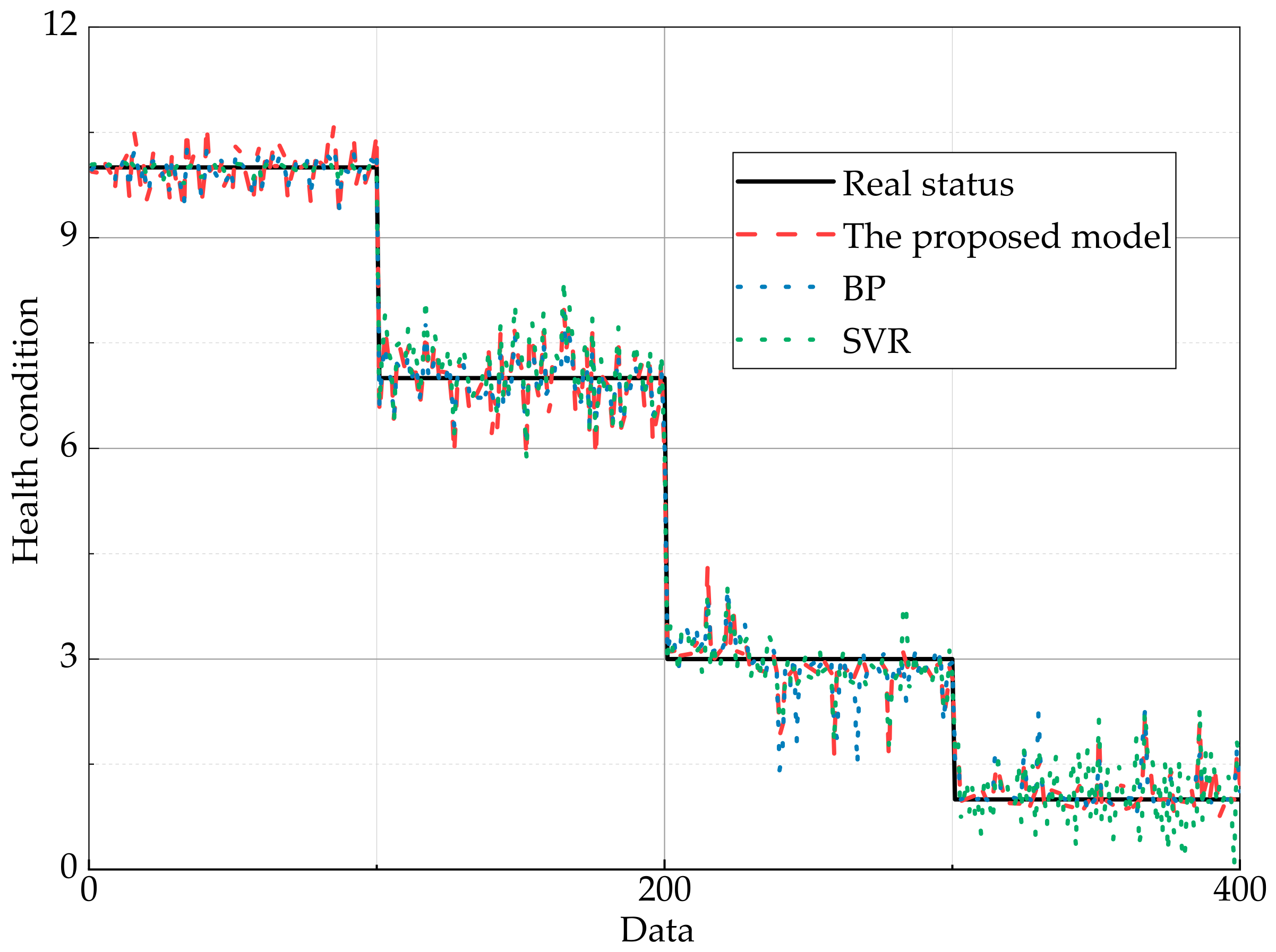
In this part, a comparative study is implemented by adopting the data-based method, including backpropagation (BP) neural network and support vector regression (SVR). Some details of BP model parameters are shown in

Table 7. The parameters of the BP models.

Method	Detail
BP Neural network	Type	Feedforward neural network
	Learning rate	0.001
	The number of layers	3
	The time of training	500
	The training goal	0.0001

. The same training data and test data are utilized. The comparison results between the simulated and actual status are shown in Figure 14.

It can be seen in Figure 14 and

Table 8. Comparison of assessment accuracy of data-based model.

Model	The Proposed Model	BPNN	SVR
RMSE	0.3500	0.3144	0.3965

, the proposed model has high accuracy, which is second only to the BP model, and the accuracy of the proposed model is improved by 6.52% compared with the SVR.

At the same time, to further compare and analyze the proposed model and BP model, 10%, 25%, 50%, and 60% of the whole data sets are randomly selected as the training set, and the whole sets of data are selected as the test set. The comparative accuracy of proposed model is calculated as follows.

As shown in

Table 9. Comparative accuracy of proposed model and BP model.

Training Data	RMSE (Proposed Model)	RMSE (BP)
10%	0.4174	0.4448
25%	0.3811	0.4162
50%	0.3500	0.3144
60%	0.3170	0.2887

, when the training set randomly selects 10% and 25% of the data set, the accuracy of the proposed model is higher than that of the BP model. While the training set randomly selects 50% and 60% of the data set, the accuracy of ER model is worse than that of the BP model. It shows that the proposed model can achieve accurate health assessment by aggregating expert knowledge and observation data in the case of less observation data and sufficient prior knowledge.

(3)

The comparison with knowledge-based models

Belief rule base (BRB) and fuzzy reasoning (FR) are the typical qualitative knowledge-based methods. In this part, BRB and FR are implemented to compare with the proposed model. Same training data and test data are selected. The initial parameters of BRB are determined by expert’ knowledge shown in

Table 10. The initial parameters of BRB model.

No.	Rule Weight	Factors		Belief Distribution of Health Status
		O	Q
1	1	H	H	(0.75, 0.10, 0.05, 0)
2	1	H	M	(0.55, 0.45, 0.05, 0)
3	0.1	H	L	(0.90, 0.10, 0, 0)
4	1	M	H	(0.60, 0.30, 0.10, 0)
5	1	M	M	(0.05, 0.30, 0.60, 0.05)
6	1	M	L	(0, 0.15, 0.35, 0.5)
7	0.1	L	H	(0.90, 0.10, 0, 0)
8	1	L	M	(0, 0.05, 0.45, 0.50)
9	1	L	L	(0, 0.05, 0.20, 0.75)

, and the part parameters of fuzzy reasoning are demonstrated in

Table 11. The parameters of FR model.

Method	Detail
Fuzzy reasoning	Initial fuzzy matrix	[0.5, 0.3, 0.2, 0; 0, 0.6, 0.3, 0.1; 0, 0, 0.5, 0.5]
	optimized fuzzy matrix	[0.75, 0.1, 0.05, 0; 1, 0, 0, 0; 0, 0.2, 0.3, 0.5]

.

It is shown in Figure 15 that the assessment results of FR and BRB are relatively scattered and far from the real status. Comparing with BRB and FR, the accuracy of the proposed model is improved by 19.28% and 16.25% respectively, as shown in

Table 12. Comparison of assessment accuracy of knowledge-based model.

Model	The Proposed Model	BRB	FR
RMSE	0.3500	0.4179	0.5058

. It is concluded that the proposed model is most accurate compared to the qualitative knowledge-based models.

5.2. Example 2—Health Assessment of Engine

In this subsection, the WD615 model engine is taken as a case to verify the effectiveness of the proposed model for complex system. The background description is introduced in Section 5.2.1. The implement progress of the proposed model is carried out in Section 5.2.2. In Section 5.2.3, the comparative study is conducted.

5.2.1. Background Description

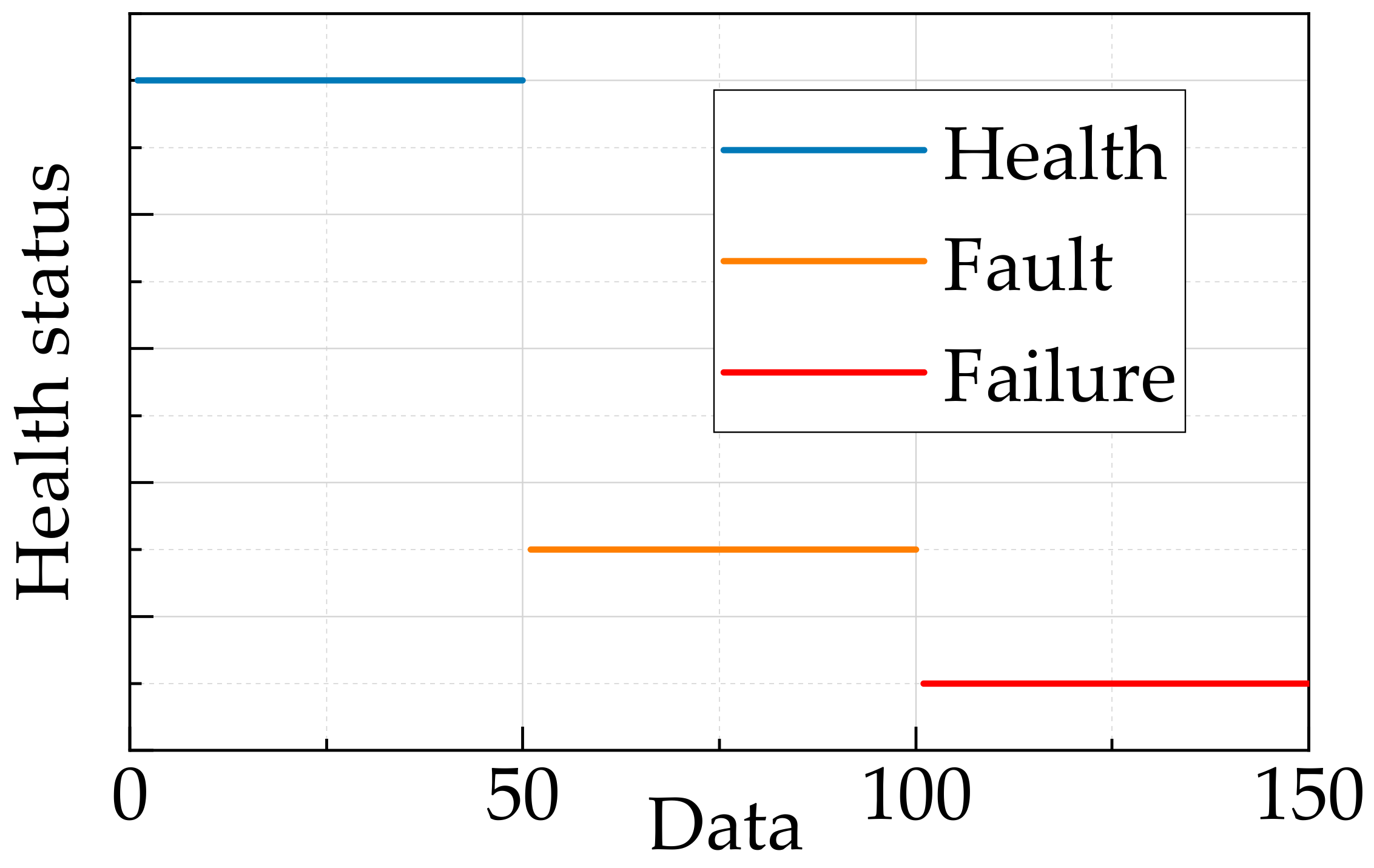
In order to monitor the operation status of engine, vibration sensors are set up for amassing the vibration signal of engine [27]. Then, the vibration signal can be processed to get the time-domain characteristics, as shown as Figure 16, Figure 17 and Figure 18. The mean, variance, and kurtosis, which reflect the center, degree of dispersion, and degree of convex of signal, are selected as the health status indicators of the engine [28]. The real status of the engine is shown in Figure 19. The assessment result grades of engine are defined as three statuses according to the different gap between the crankshaft and bearing connecting rod: First, a gap of 0.08 mm to 0.1 mm belongs to “Health”; a gap of 0.18 mm to 0.2 mm belongs to “Fault”; a gap of 0.32 mm to 0.34 mm belongs to “Failure”. Thus, a frame of discernment Φ is defined as follows.

$$\Phi =\{Health, Fault, Failure{\}=\{\mathrm{D}}_1, {\mathrm{D}}_2, {\mathrm{D}}_3\}$$

(36)

There are 150 sets of data, including the status of “Health”, “Fault”, and “Failure”. The mean of vibration signal ranges from 0.802 to 0.1761. The variance of vibration signal ranges from 0.0038 to 0.0191, and the kurtosis of vibration signal ranges from 2.2159 to 7.6801 as shown in Figure 16, Figure 17 and Figure 18, respectively.

5.2.2. Construction and Optimization of Assessment Model

To construct a health assessment model of engine, first the indicators reference grades are determined as follows.

$$H_{mean}=H_{variance}=\{Small, Medium, Slight l\arg e, L\arg e\}=\{S,M,SL,L\}$$

(37)

$$H_{kurtosis}=\left\{Average, High\right\}=\{A,H\}$$

(38)

where $H_{mean}$, $H_{variance}$, and $H_{kurtosis}$ denote the reference grades of mean, variance, and kurtosis.

Due to the reference grades are disaccord with assessment result grades, transformation matrixes are introduced to transform input information, and the initial values of transformation matrix and reference values are determined based on expert’s knowledge in

Table 13. The initial values of transformation matrix.

No.	Indicators	Reference Values	Belief Distribution
1	Mean	0.08	(0.90, 0.10, 0.00)
2		0.10	(0.85, 0.10, 0.05)
3		0.14	(0.15, 0.45, 0.40)
4		0.18	(0.05, 0.15, 0.75)
5	Variance	0.003	(0.70, 0.25, 0.05)
6		0.01	(0.35, 0.50, 0.15)
7		0.013	(0.05, 0.20, 0.75)
8		0.020	(0.00, 0.25, 0.75)
9	Kurtosis	2	(0.70, 0.20, 0.10)
10		8	(0.00, 0.30, 0.70)

.

The Table 13 can be expressed as a form of matrix as Formulas (39) and (40). Then, the initial evidence is given by using the rule-based transformation technique. According to the implement process of example 1 in Section 5.1, the optimized simulated status is introduced in Figure 18. In the process of optimization, 75 sets of data are selected alternately from 150 sets of data as training data, and the whole sets of data are taken as test data.

$$A_1=\left[\begin{array}{cccc}0.9& 0.85& 0.15& 0.05\\ 0.1& 0.1& 0.45& 0.15\\ 0& 0.05& 0.4& 0.75\end{array}\right]$$

(39)

$$A_2=\left[\begin{array}{cccc}0.7& 0.35& 0.05& 0\\ 0.25& 0.5& 0.2& 0.25\\ 0.05& 0.15& 0.75& 0.75\end{array}\right],A_3=\left[\begin{array}{cc}0.7& 0\\ 0.2& 0.3\\ 0.1& 0.7\end{array}\right]$$

(40)

It is shown in Figure 20 that contrasting with the optimized simulated status, the error between the initial status and real status is rather large, especially in the first and third stages. By calculating the root mean square, the accuracy of the optimized status is 41.7% higher than the initial status. The optimized and calculated model parameters are given in

Table 14. The parameters of optimized model parameters.

Parameters	Values
indicators	Mean	Variance	Kurtosis
weight	0.7329	0.7950	0.922
reliability	0.8491	0.835	0.935
Health status	Health	Fault	Failure
Expected utility	10.123	4.893	0.277

and

Table 15. The optimized transformation matrix.

No.	Indicators	Reference Values	Belief Distribution
1	Means	0.0801	(0.959, 0.040, 0.001)
2		0.116	(0.972, 0.027, 0.001)
3		0.131	(0.106, 0.327, 0.567)
4		0.178	(0.129, 0.212, 0.659)
5	Variance	0.0031	(0.527, 0.466, 0.070)
6		0.0090	(0.503, 0.496, 0.001)
7		0.0126	(0.060, 0.275, 0.665)
8		0.0193	(0.010, 0.451, 0.539)
9	Kurtosis	1.758	(0.679, 0.224, 0.096)
10		7.720	(0.002, 0.423, 0.575)

.

5.2.3. Comparative Study

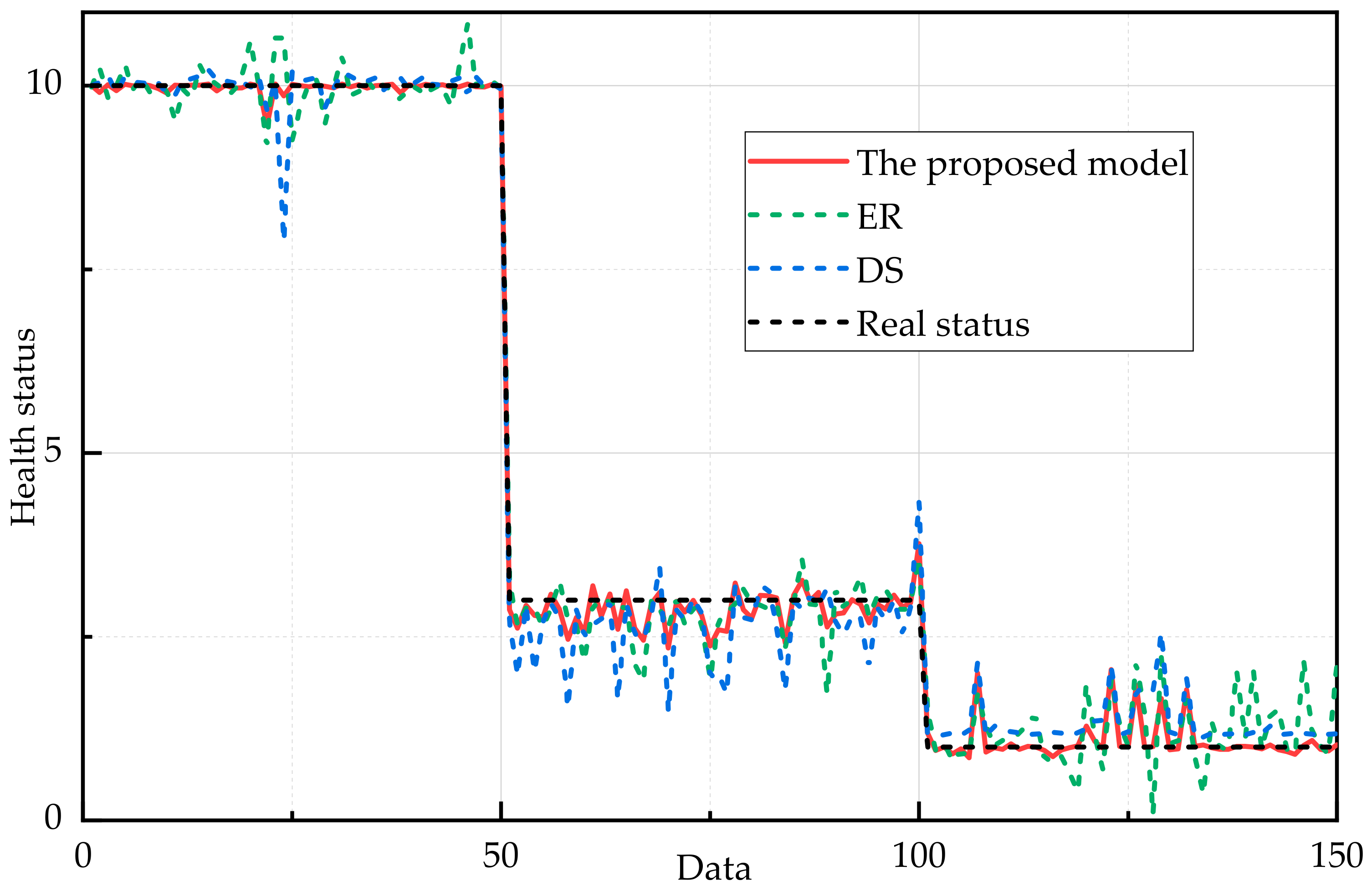
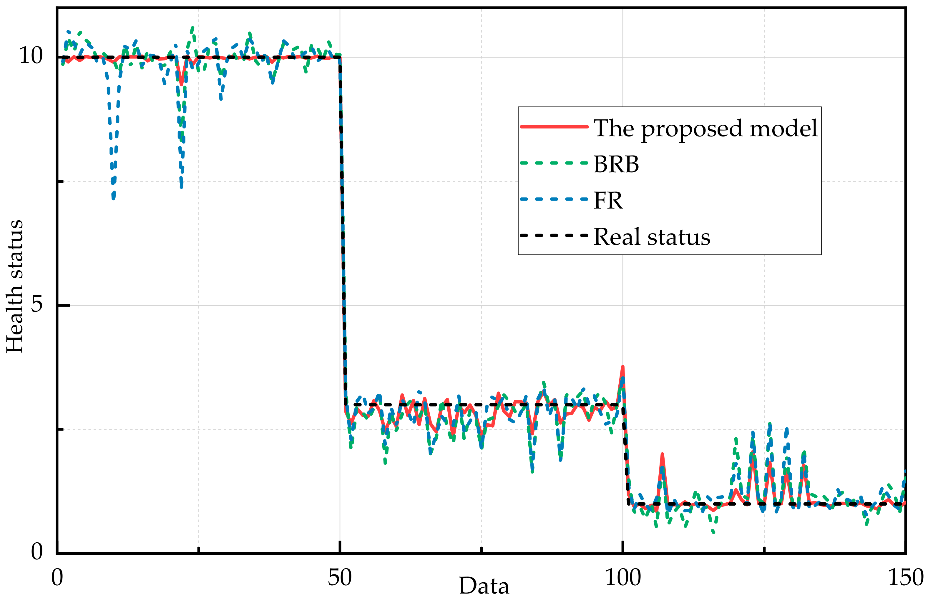
In this subsection, based on the same training data and test data, several kinds of qualitative knowledge-based models and data-based models are employed to compare with the proposed model.

It can be seen in the Figure 21, Figure 22 and Figure 23 that the performance of the proposed model is better than other methods, and its assessment accuracy is improved by 10.4%, 20.6%, 8.9%, 14.4%, 15.9%, and 27.6% compared to ER, DS, BP, SVR, BRB, and FR, respectively shown in

Table 16. Comparison of different models.

Model	The Proposed Model	ER	DS	BP	SVR	BRB	FR
RMSE	0.3730	0.4162	0.4695	0.4098	0.4355	0.4436	0.5154

.

5.3. Result Analysis

In the above two examples, the health status of the bus of control system and engine is assessed by the proposed model, where the input indicators reference grades disaccord with the assessment result grades are fully considered, and include three situations: (1) the indicators reference grades are more than the assessment result grades, (2) the input indicators reference grades are less than the assessment result grades, (3) above cases exist simultaneously. According to the above comparative research, it can be proved that the proposed method is able to combine the advantage of both data-based methods and qualitative knowledge-based method, providing an interpretable and accurate assessment result for decision-makers.

In fact, those two examples provide a general process to solve the inconsistent problem between input and output. More importantly, the proposed method can not only be applied in these two cases, but also can be extended to the dynamic assessment and other multiple indicators of health assessment.

6. Conclusions

An ER rule-based health assessment model for a complex system is proposed, where the transformation matrix is considered. In addition, case study of the bus of control system and the engine is investigated to demonstrate the validity and practicality of the proposed method.

There are mainly two contributions of this paper. First, the transformation matrix is employed to solve the disaccord problem between the input indicator reference grades and assessment result grades, which keeps the consistency and completeness of the possession of the input information transformation. Second, the calculation methods of indicator weight and reliability are conducted, where the qualitative knowledge and quantitative information are fully used. Then, the optimization method of the model is conducted, and a complete health assessment model is constructed.

According to the proposed model, the future research work can be summarized into the following two points:

(1) In engineering practice, the forms of health status threshold can be various, and the forms are not only numerical, but can also be in interval form or normal distribution form. Therefore, how to solve the disaccord problem between the indicators reference grades and assessment result grades under the different forms of threshold should be addressed.

(2) The integration model between deep learning and ER rule can be established based on the good uncertainty processing ability and interpretability of ER rule.

References

- Duan, Z.; Sun, H.; Wu, C.; Hu, H.; Hu, H. Flow-network based dynamic modelling and simulation of the temperature control system for commercial aircraft with multiple temperature zones. Energy 2022, 238, 121874. [Google Scholar] [CrossRef]
- Yi, T.; Jin, C.; Gao, L.; Hong, J.; Liu, Y. Nested Optimization of Oil-Circulating Hydro-Pneumatic Energy Storage System for Hybrid Mining Trucks. Machines 2022, 10, 22. [Google Scholar] [CrossRef]
- Gao, Q. Nonlinear Adaptive Control with Asymmetric Pressure Difference Compensation of a Hydraulic Pressure Servo System Using Two High Speed on/off Valves. Machines 2022, 10, 66. [Google Scholar] [CrossRef]
- Liu, Y.; Xu, J.; Yuan, H.; Lv, J.; Ma, Z. Health Assessment and Prediction of Overhead Line Based on Health Index. IEEE Trans. Ind. Electron. 2019, 66, 5546–5557. [Google Scholar] [CrossRef]
- Zhou, T.; Wu, W.; Peng, L.; Zhang, M.; Li, Z.; Xiong, Y.; Bai, Y. Evaluation of urban bus service reliability on variable time horizons using a hybrid deep learning method. Reliab. Eng. Syst. Saf. 2022, 217, 108090. [Google Scholar] [CrossRef]
- Miao, H.; Li, B.; Sun, C.; Liu, J. Joint Learning of Degradation Assessment and RUL Prediction for Aeroengines via Dual-Task Deep LSTM Networks. IEEE Trans. Ind. Inform. 2019, 15, 5023–5032. [Google Scholar] [CrossRef]
- Li, Z.; Wu, J.; Yue, X. A Shape-Constrained Neural Data Fusion Network for Health Index Construction and Residual Life Prediction. IEEE Trans. Neural Netw. Learn. Syst. 2021, 32, 5022–5033. [Google Scholar] [CrossRef]
- Salamai, A.; Hussain, O.; Saberi, M. Decision Support System for Risk Assessment Using Fuzzy Inference in Supply Chain Big Data. In Proceedings of the 2019 International Conference on High Performance Big Data and Intelligent Systems (HPBD&IS), Shenzhen, China, 9–11 May 2019; pp. 248–253. [Google Scholar] [CrossRef]
- Zhu, L. An MI-BRB Based Health State Assessment Methodology for Running Gears in High-Speed Trains. In Proceedings of the 2020 3rd World Conference on Mechanical Engineering and Intelligent Manufacturing (WCMEIM), Shanghai, China, 4–6 December 2020; pp. 768–772. [Google Scholar] [CrossRef]
- Bjornsen, K.; Selvik, J.T.; Aven, T. A semi-quantitative assessment process for improved use of the expected value of information measure in safety management. Reliab. Eng. Syst. Saf. 2019, 188, 494–502. [Google Scholar] [CrossRef]
- Yang, J.B.; Xu, D.L. Evidential reasoning rule for evidence combination. Artif. Intell. 2013, 205, 1–29. [Google Scholar] [CrossRef]
- Dempster, A. A Generalization of Bayesian Theory. J. R. Stat. Soc. Ser. B Methodol. 1968, 30, 205–247. [Google Scholar]
- Xu, D.L. On the evidential reasoning algorithm for multiple attribute decision analysis under uncertainty. IEEE Trans. Syst. Man Cybern.—Part A Syst. Hum. 2002, 32, 289–304. [Google Scholar]
- Yang, J.B.; Pratyush, S. A general multi-level evaluation process for hybrid MADM with uncertainty. IEEE Trans. Syst. Man Cybern. 1994, 24, 1458–1473. [Google Scholar] [CrossRef] [Green Version]
- Zhang, Z.; Liao, H.; Tang, A. Renewable energy portfolio optimization with public participation under uncertainty: A hybrid multi-attribute multi-objective decision-making method. Appl. Energy 2022, 307, 118267. [Google Scholar] [CrossRef]
- Ning, P.; Zhou, Z.; Cao, Y.; Tang, S.; Wang, J. A Concurrent Fault Diagnosis Model via the Evidential Reasoning Rule. IEEE Trans. Instrum. Meas. 2022, 71, 1–16. [Google Scholar] [CrossRef]
- Zhang, C.; Zhou, Z.; Hu, G.; Yang, L.; Tang, S. Health assessment of the wharf based on evidential reasoning rule considering optimal sensor placement. Measurement 2021, 186, 110184. [Google Scholar] [CrossRef]
- Xiong, Y.; Jiang, Z.; Fang, H.; Fan, H. Research on Health Condition Assessment Method for Spacecraft Power Control System Based on SVM and Cloud Model. In Proceedings of the 2019 Prognostics and System Health Management Conference (PHM-Paris), Paris, France, 2–5 May 2019; pp. 143–149. [Google Scholar] [CrossRef]
- Tao, J.; Wang, X.; Liang, X. Health State Evaluation for Fuzzy Multi-state Production Systems based on MPNM. In Proceedings of the 2020 11th International Conference on Prognostics and System Health Management (PHM-2020 Jinan), Jinan, China, 23–25 October 2020; pp. 5–10. [Google Scholar] [CrossRef]
- Yang, J.B. Rule and utility based evidential reasoning approach for multiattribute decision analysis under uncertainties. Eur. J. Oper. Res. 2001, 131, 31–61. [Google Scholar] [CrossRef]
- Yang, J.B.; Singh, M.G. An evidential reasoning approach for multiple-attribute decision making with uncertainty. IEEE Trans. Syst. Man Cybern. 1994, 24, 1–18. [Google Scholar] [CrossRef] [Green Version]
- Feng, Z.C.; Zhou, Z.; Hu, C.; Chang, L.; Hu, G.; Zhao, F. A new belief rule base model with attribute reliability. IEEE Trans. Fuzzy Syst. 2019, 27, 903–916. [Google Scholar] [CrossRef]
- Zhao, F.; Zhou, Z.; Hu, C.; Chang, L.; Li, G. A new evidential reasoning-based method for online safety evaluation of complex systems. IEEE Trans. Syst. Man Cybern. Syst. 2018, 48, 954–966. [Google Scholar] [CrossRef]
- Stan, O.; Cohen, A.; Elovici, Y.; Shabtai, A. Intrusion Detection System for the MIL-STD-1553 Communication Bus. IEEE Trans. Aerosp. Electron. Syst. 2020, 56, 3010–3027. [Google Scholar] [CrossRef]
- Wang, D.; Xu, Y.; Li, J.; Zhang, M.; Li, J.; Qin, J.; Chen, X. Comprehensive Eye Diagram Analysis: A Transfer Learning Approach. IEEE Photonics J. 2019, 11, 1–19. [Google Scholar] [CrossRef]
- Zhao, Y.; Tang, Y.; Xiao, J.; Mou, W. Eye Diagram Analysis Based on System View-Taking PCM System as an Example. In Proceedings of the 2020 5th International Conference on Mechanical, Control and Computer Engineering (ICMCCE), Harbin, China, 25–27 December 2020; pp. 2286–2289. [Google Scholar] [CrossRef]
- Wang, M.; Qin, G.; Chen, J.; Liao, Y. Design of Vibration Monitoring and Fault Diagnosis System for Marine Diesel Engine. In Proceedings of the 2020 11th International Conference on Prognostics and System Health Management (PHM-2020 Jinan), Jinan, China, 23–25 October 2020; pp. 1–4. [Google Scholar] [CrossRef]
- Liu, Y.; Chang, W.; Zhang, S.; Zhou, S. Fault Diagnosis and Prediction Method for Valve Clearance of Diesel Engine Based on Linear Regression. In Proceedings of the 2020 Annual Reliability and Maintainability Symposium (RAMS), Palm Springs, CA, USA, 27–30 January 2020; pp. 1–6. [Google Scholar] [CrossRef]
Figure 1.
The structure of the health assessment model.
Figure 2.
The transformation between the input and output.
Figure 3.
Optimization process of model parameters.
Figure 4.
The implementation process of the assessment model.
Figure 5.
Simulation model of bus of control system.
Figure 6.
Observation data of O and Q.
Figure 7.
The health status of the bus of control system.
Figure 8.
Belief distribution of O.
Figure 9.
Belief distribution of Q.
Figure 10.
The aggregated health status.
Figure 11.
The comparison between initial and real status.
Figure 12.
The comparison between the optimized model and initial model.
Figure 13.
The comparison under ER rule framework.
Figure 14.
The comparison of data-based models.
Figure 15.
Comparison of qualitative knowledge-based models.
Figure 16.
The mean of vibration signal.
Figure 17.
The variance of vibration signal.
Figure 18.
The kurtosis of vibration signal.
Figure 19.
The health status of engine.
Figure 20.
The comparison between the initial and optimized status.
Figure 21.
The comparison under ER framework.