
Fault Prediction of Rolling Element Bearings Using the Optimized MCKD–LSTM Model


1
College of Mechanical Engineering, Xinjiang University, Urumqi 830047, China
2
Changsha Institute of Mining Research Co., Ltd., Changsha 410012, China
*
Authors to whom correspondence should be addressed.
Machines 2022, 10(5), 342; https://0-doi-org.brum.beds.ac.uk/10.3390/machines10050342
Submission received: 22 March 2022
/
Revised: 26 April 2022
/
Accepted: 3 May 2022
/
Published: 6 May 2022
(This article belongs to the Topic Artificial Intelligence in Smart Industrial Diagnostics and Manufacturing)
Abstract
:The reliability and safety of rotating equipment depend on the performance of bearings. For complex systems with high reliability and safety needs, effectively predicting the fault data in the use stage has important guiding significance for reasonably formulating reliability plans and carrying out reliability maintenance activities. Many methods have been used to solve the problem of reliability prediction. Due to its convenience and efficiency, the data-driven method is increasingly widely used in practical reliability prediction. In order to ensure the reliability of bearing operation, the main objective of the present study is to establish a novel model based on the optimized maximum correlation kurtosis deconvolution (MCKD) and long short-term memory (LSTM) recurrent neural network to realize early bearing fault warnings by predicting bearing fault time series. The proposed model is based on the lifecycle vibration signal of the bearing. In the first step, the cuckoo search (CS) is utilized to optimize the parameter filter length and deconvolution period of MCKD, considering the influence of periodic bearing time series, and to improve the fault impact component of the optimized MCKD deconvolution time series. Then the LSTM learning rate is selected according to the deconvolution time series. Finally, the dataset obtained through various preprocessing approaches is used to train and predict the LSTM model. The analyses performed using the XJTU-SY bearing dataset demonstrate that the prediction results are in good consistency with real fault data, and the average prediction accuracy of the optimized MCKD–LSTM model is 26% higher than that of the original time series.
1. Introduction
Rolling element bearing, which is also called “industrial joint”, has been widely used in diverse engineering fields, including transmission and hoisting, wind power generation, and aerospace [1,2,3]. Since bearings are among the core components of rotating equipment, it is of significant importance to investigate and predict bearing faults [4,5,6]. Studies show that bearing performance directly affects the reliability and safety of heavy machinery. Accordingly, accurate prediction of fault time series in bearings is an essential factor in achieving safe industrial production [7,8,9].
Currently, the bearing-fault time series is created using the convolution of vibration signals and different noise signals in the signal transmission process. However, this method affects the accuracy of the prediction model after training. In order to resolve this problem, the first part of this study is dedicated to preprocessing the original time series. In this regard, Dong et al. [10] combined the spectral wavelet transform, detrended fluctuation analysis and proposed a non-iterative denoising method to filter nonlinear vibration signals. Moreover, Yan et al. [11] explored the discrete convolution wavelet transform (DCWT) to decompose and reconstruct signals in signal processing of swiftly changing signals. Although remarkable achievements have been realized, the selection capacity of the wavelet-based function is severely limited [12]. Sharma and Parey [13] employed the variational mode decomposition (VMD) to handle the multi-component modulated non-stationary vibration signal of the transmission. To discover the modal properties of engineering structures, Bagheri et al. [14] proposed a dynamic response decomposition scheme based on the VMD. Furthermore, Zhang et al. [15] investigated the fractal properties of vibration signals of rolling element bearings and developed an effective method to assess and diagnose the bearing defects. Further investigations revealed that the decomposition mode parameter K and the penalty coefficient η have a significant impact on the decomposition effect, and should be established to solve the varying parameters. To alleviate the mode mixing of complicated vibration signals, Zhao X et al. [16] proposed an approach based on the single-objective salp swarm algorithm to optimize the penalty coefficient η of the VMD. Feng et al. [17] used the whale optimization algorithm (WOA) to optimize VMD parameters, achieve adaptive decomposition, and reduce noise in vibration signals. On the other hand, the decomposition parameters of VMD should be set according to the properties of the signal. More specifically, selecting inappropriate parameters may result in over-decomposition and under-decomposition [18]. McDonald et al. [19] established maximum correlated kurtosis deconvolution (MCKD), which is an ideal method to process early bearing fault signals with low signal-to-noise ratio and periodic impact characteristics [20]. To achieve composite fault diagnosis, Hong et al. [21] used adaptive MCKD to decouple the fault information and the noise-reduction signal. Zhang et al. [22] suggested a signal noise-reduction method based on the Teager energy operator and the MCKD. Recently, the filter length L and the shift order M in the MCKD have been optimized accordingly. Lyu et al. [23] optimized the filter length and deconvolution period of the MCKD for composite fault diagnosis of gear-tooth wear and bearing outer-ring fault using the quantum genetic algorithm (QGA). To achieve bearing composite fault diagnosis and estimate the prior period T, Miao et al. [24] used the autocorrelation of the envelope signal. To obtain the best noise-reduction performance and select the filter length L using MCKD, Yang et al. [25] applied permutation entropy as the measurement index.
In order to develop a bearing-fault time series prediction model, Pan et al. [26] calculated the upper and lower boundaries of unknown elevation on a terrain profile using the double multiplicative neuron (DMN) model and the modified particle swarm optimization (MPSO) technique. Moreover, Raubitzek and Neubauer [27] presented a fractal interpolation method to predict the time series. For long-term time series prediction, Liu et al. [28] proposed dual-stage two-phase (DSTP)-based RNN (DSTP-RNN) and DSTP-RNN-Ⅱ algorithms. Savad koohi et al. [29] predicted the human fall risk using the depth neural network model. Meanwhile, Zhang et al. [30] introduced high-level abstract features into an LSTM network and proposed the CEEMD-PCA-LSTM hybrid prediction model to predict time series. Che et al. [31] proposed the 1d-CNN model for regression analysis of time series samples, and then employed bidirectional long short-memory (Bi-LSTM) to establish a performance-deterioration model and predict the performance decline over time. Recently, Niu and Yang [32] proposed Dempster–Shafer regression technology to predict time series in diverse problems.
Based on the literature survey, the main objective of the present study is to take the strong noise-reduction effect of the MCKD in periodic signals to denoise the bearing-fault time series and acquire the deconvolution time series. Then the deconvolution time series are used to train long short-term memory recurrent neural networks and establish the optimized MCKD–LSTM prediction model to predict the bearing-fault time series.
This article is organized as follows: Section 2 reviews the relevant methods. In Section 2.1,the basics of maximum correlated kurtosis deconvolution in signal processing are reviewed and the performance of noisy sample reconstruction is analyzed. Then parameters of the CS optimization are introduced in Section 2.2. The long short-term memory recurrent neural network for predicting bearing-fault time series is introduced in Section 2.3. The cuckoo search for optimizing MCKD is analyzed in Section 3. The effectiveness of LSTM in predicting the fault time series of bearing signals is verified experimentally in Section 4. Finally, the main achievements and conclusions are summarized in Section 5.
2. Correlation Method
2.1. Maximum Correlated Kurtosis Deconvolution
Mcdonald et al. [19] proposed maximum correlated kurtosis deconvolution (MCKD) and successfully applied this method in gear-flaking fault diagnosis by considering the impact and periodic characteristics of the fault information. In this algorithm, y represents the impulse signal, h is the response of the y signal after passing the transmission path, and x denotes the signal convoluted from various signals on the transmission path. The mathematical correlation between these parameters can be expressed as follows:
The main objective of MCKD is to find a finite impulse response (FIR) filter to solve the input signal y through the output signal x. This can be expressed as follows:
where f = [f1,f2,…,fL]T is the filter factor of the length L.
In MCKD, the maximum correlation kurtosis is considered as the evaluation criterion:
In order to obtain the optimal inverse filter coefficient f, the first derivative of the objective function should become zero.
Consequently, the optimum filter coefficient can be obtained in the form below:
The main steps to realize MCKD are as follows:
- (1)
- Determine the filter length L, the order of shift M, and period T of the impact signal.
- (2)
- Calculate X0 and matrices of the original signal x(n).
- (3)
- Obtain the filtered output signal y(n).
- (4)
- Calculate αm and β according to y(n).
- (5)
- Update the filter coefficient f.
If the signal f before and after filtering conforms to the condition, the iteration ends, and the calculation continues from step (3).
The deconvolution signal y of the actual acquisition signal x can be obtained by substituting the obtained inverse filter coefficients.
2.2. Cuckoo Search
The cuckoo search [33] refers to a heuristic search algorithm that integrates the Lévy flights theory with the parasitic behavior of cuckoos. It has superior characteristics, including few parameters and fast convergence. The cuckoo search consists of the following three ideal rules:
- (1)
- Each cuckoo lays only one egg at a time and places the eggs in a randomly selected nest, which is also known as a host nest.
- (2)
- The parasitic nest with the highest quality eggs will be retained for the next generation.
- (3)
- The number of possible nests is fixed, and the chance of discovering host eggs in a nest is p.
When the host bird discovers the host egg, it either throws it out or abandons the nest to establish a new one in a new site.
After randomly generating n nest placements, a new nest location is established using the Lévy flights search strategy. This can be mathematically expressed as follows:
where Xw+1i and Xwi signify the ith cuckoo’s nest site in the w and w + 1 generations, respectively. Moreover, Xwb is the optimal nest location in the current search. The parameter α0 reflects the step size. In the present study, the step size is set to α0 = 0.01. µ and ν are random values generated using the normal distribution, and the default value of H is 0.5.
During the calculations, the nest with the higher fitness value is kept when the new nest location is found using the Lévy flight search strategy. Then, based on the discovery probability p, a number of the nest positions are eliminated, and a new nest position is constructed using the preferred random walk search strategy. This can be expressed as follows:
where r is a random number between 0 and 1, and Xwj and Xwk are two candidate solutions that are randomly selected from the current population.
2.3. Long Short-Term Memory Recurrent Neural Network
In this section, the gating mechanism is employed in the long short-term memory (LSTM) recurrent neural network [34]. It is worth noting that this mechanism has been frequently used to process time series signals. LSTM can be mathematically expressed as follows:
2.3.1. Forward Calculation Method of LSTM
Figure 1 indicates that for a given time series signal x = (x1, x2, …, xt) and a hidden layer sequence ht−1 = (h1, h2, …, ht−1), the candidate state value , input gate value it, forgetting gate value ft, output gate value ot, memory cell value ct, hidden layer sequence ht, and the output sequence yt = (y1, y2,…, yt) at time t can be determined using the conventional LSTM model.
2.3.2. Reverse Computation Method of LSTM
The calculations of the LSTM training algorithm can be mainly summarized in the following four steps:
- (1)
- The output value of each neuron is calculated forward f(y) = f(wTx)
- (2)
- The cost function is the mean square deviation function J, and the error term δj value of each neuron is calculated inversely as follows:
- (3)
- Reverse error gradient calculation from the following expression:
- (4)
- Determine the weight difference Δw:
In the present study, the mean square error (MSE) is used as the measuring standard to evaluate the accuracy of the prediction model. By calculating the MSE of the training and test sets, the fitting and prediction accuracy of the model can be analyzed quantitatively.
3. Parameter Optimization Based on the Cuckoo Search
As shown in Figure 2, due to noise generation inherent to the operation of rotating systems under industrial environments, it is necessary to preprocess the bearing data before predicting the bearing-fault time series, so as to further improve the prediction accuracy of bearing-fault time series. Typically, because the bearing signal has both periodicity and impact, the fault signal and noise can be effectively separated using this characteristic. The main reason for choosing MCKD is that it takes the maximization of correlation kurtosis as the evaluation standard, and its essence is to find a final impulse response (FIR) filter. From this process, it can be observed that MCKD takes into account the periodicity and impact of fault signal to denoise. When utilizing MCKD to denoise bearing-fault time series, specific hyperparameters [L, T] must be adjusted to achieve optimal performance. Classically, in the relevant condition-monitoring reference, this process is addressed in an empirical manner to maximize the final diagnostic performance. However, this method leads to a high risk of over-fitting; that is, MCKD is forced to give priority to those modes that provide higher diagnostic performance, rather than those that better describe the original signal according to the reconstructed fitness function. On the other hand, in most cases, several hyperparameter-tuning strategies are classically proposed to optimize the hyperparameter for a single model criterion and obtain a high-performance model. In this sense, the challenge of the proposal is to realize the hyperparameter adjustment program by considering the impact of highlighting the fault signal. Therefore, a heuristic search algorithm, cuckoo search (CS), is used to adjust the hyperparameter of MCKD, in which the fitness function of CS is focused on maximizing the crest factor of envelope spectrum (Ec) in the reconstruction process.
When using CS to optimize the parameters, it is important to choose the right fitness function based on the signal characteristics and the periodic impact signal of the bearing signal, which may differ from the noise signal. In this regard, Zhang et al. [35] proposed a dimensionless crest factor of the envelope spectrum (Ec) index that takes into consideration the periodic properties of fault information in vibration signals. Assuming the signal envelope spectrum amplitude X(j) (j = 1, 2,…, M), the index Ec can be defined as follows:
where emax is the highest value of the envelope signal obtained after Hilbert demodulation in the range [n × fr, fs/2], fr is the bearing signal’s frequency conversion, and fs is the sampling frequency. Moreover, erms denotes the effective value, which is defined as the effective value of the signal following the Hilbert demodulation. In the present study, rotating frequency multiple of bearing is set to n = 2 to prevent the influence of fr on Ec.
It should be indicated that the envelope spectrum peak factor Ec of the envelope signal acquired by the Hilbert demodulation is determined using the MCKD operation on the fault signal in an arbitrary nest Xi location. Therefore, Ec reflects the fitness value of the bird nest. When the periodic impact occurs in the decomposition results, the envelope spectrum peak factor Ec is significant and the decomposition effect is optimal. On the other hand, for a relatively small envelope spectrum peak factor Ec, the decomposition effect is negligible. Accordingly, the greatest value of Ec is considered as the optimization object.
In fact, according to [36], heuristic search algorithms, such as CS, have been widely used and preferred, because the solution is based on random optimization method. In addition, one of the main advantages of utilizing CS is that it is simple and easy and does not need a large number of parameters to solve the problem, because for the optimization algorithm itself, fewer parameters can allow researchers to spend less time finding the best combination of parameters. Secondly, the experimental results are compared by testing examples, such as standard test functions; this shows that the results of CSare superior to those of genetic algorithm (GA) and particle swarm optimization (PSO)algorithm, and has also have greater robustness.
Finally, the LSTM neural network is a good method to deal with time series. The function of an LSTM memory unit is to make the information flow effectively. Considering the data characteristics of finite sample points of univariate fault time series and the design principle of simplifying recurrent neural network, the overall framework of the LSTM prediction model constructed in this paper is shown in Figure 2, including five functional modules: input layer, hidden layer, output layer, network training, and network prediction. The input layer is responsible for the preliminary processing of the original fault time series to meet the network input requirements. The hidden layer uses the LSTM cells shown in Figure 1 to build a single-layer recurrent neural network, and the output layer provides the prediction results. The network training adopts the random gradient descent optimization method mentioned in Section 2.3.2, and the network prediction adopts the iterative method to predict point by point. Figure 2 shows the flowchart of the proposed fault diagnosis method.
4. Experimental Signal Analysis
To analyze the obtained results, the experimental dataset of the LDK UER204 rolling element bearings of XJTU–SY bearing [37] were used. Figure 3 illustrates the configuration of the bearing accelerated life testbed and outer-ring crack of a bearing. During the experiment, two unidirectional acceleration sensors (PCB 352C33, PCB Piezotronics, New York, NY, USA) were installed along the vertical and horizontal directions to collect vibration signals through a portable dynamic signal collector (Measurement Computing Corporation, Norton, MA, USA). The sampling frequency and the sampling interval were set to 25.6 kHz and 1 min, respectively, and 32,769 samples were taken in total. Then the horizontal vibration signals in the dataset bearing1_1 were selected to perform the analysis.
4.1. Data Preprocessing
The vibration signal of the 50th series along the horizontal direction of the bearing1_1 was selected to predict the bearing-fault time series. Figure 4 illustrates the time-frequency domain diagram of a vibration signal. It can be observed that there are many impact components to consider in the temporal domain, while no clear rule has yet been enacted. The frequency spectrum shows the frequency conversion of 34.38 Hz and its frequency doubling components, and several resonance frequency bands appear in the high–frequency band. It was found that the frequency components were complex, and the bearing outer-ring fault had no distinct frequency. Consequently, it was necessary to retrieve the time series in order to access more impact information to denoise the original time series.
In the present study, the MCKD was used to preprocess the original time series while the order of the shift M and the iteration termination times G were set to 1 and 20, respectively. Meanwhile, the CS was used to optimize the filter length L and deconvolution period T. The main parameters of the CS were set as follows: the dimension of solution D was set to 2, the population size N was set to 15, the host bird with probability P was set to 0.1. Furthermore, the upper and lower bounds were searched based on L > 2fs/fc and T = fs/fc [38], where fs is the sampling frequency and fc denotes the characteristic frequency. In all calculations, the optimization ranges were set to L = [100, 1500] and T = [50, 1000]. Figure 5a shows the results, indicating that the peak factor of the local maximum envelope spectrum converged to 10.2478 at the 7th iteration, and the corresponding optimization parameter combination [L, T] to the peak factor of the local maximum envelope spectrum was [600, 235]. Then the original time series signal was denoised using the MCKD parameters to obtain the deconvolution series signal and envelope spectrum. The obtained results in Figure 5b,c demonstrate that the impact component intensity of the deconvolution series signal increased in the time domain. Moreover, the noise interference component reduced significantly, the frequency conversion component approached 34.38 Hz, 108.6 Hz, and frequency doubling emerged in the envelope spectrum. This frequency was consistent with the theoretical value of the bearing outer–ring crack characteristic frequency of 107.91 Hz, resulting in a significant noise reduction.
The deconvolution time series were then taken as one dimensional time series to train the prediction model of the bearing fault time series. All one dimensional vibration signals were selected at once based on the 50th original time series every ten series. Among 102 groups of time series, six groups were taken as the training set, and seven groups were taken as the test set. Meanwhile, the optimized MCKD was utilized to denoise. After the whole dataset was established, it was introduced to the LSTM model to train the model and predict bearing fault time series.
To evaluate the performance of the optimized MCKD–LSTM in predicting the bearing fault time series, the original fault series were denoised using EMD and optimized VMD. Training of the LSTM model was then completed, and it was compared with the predictions of the bearing fault time series. Figure 6 reveals that since the impact signal is included in the bearing lifecycle signal, the fault impact information of the bearing will appear in partial IMF components after signal processing by EMD; hence the kurtosis diagram shows ten IMF components, IMF1 to IMF10. In the present study, the five components with the highest kurtosis (i.e., IMF9, IMF6, IMF1, IMF2, and IMF10) were chosen as one dimensional time series to rearrange the signal. Both the training and test sets are EMD processed simultaneously.
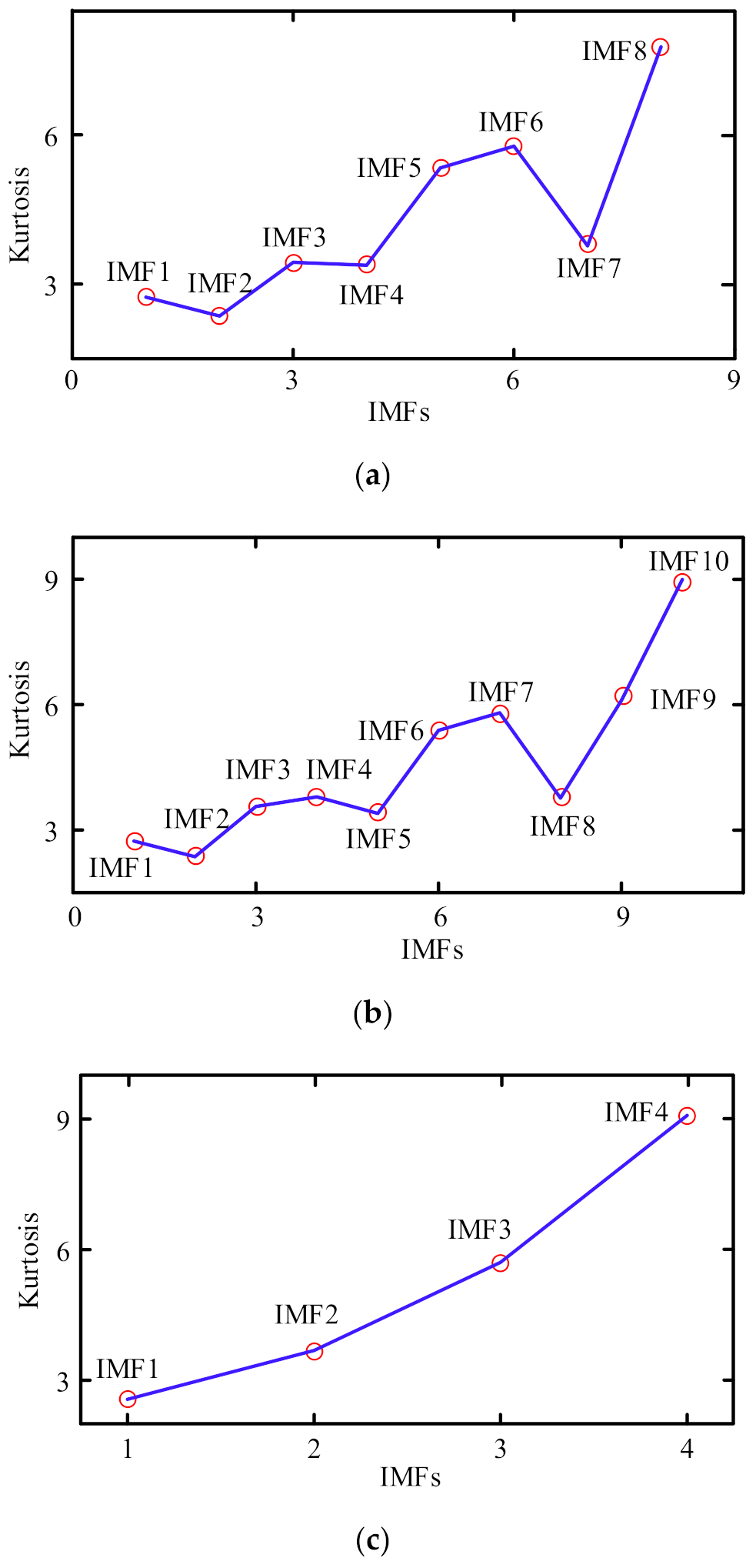
Similarly, VMD is applied to denoise the dataset. However, the decomposition mode parameter K and the penalty term coefficient α should be considered in the signal analysis. Generally, the central frequency observation [39] and EMD–VMD methods can be used to select the decomposition mode parameter K. In this case, the correlation between the K–value and the penalty term coefficient α can be ignored. Moreover, the CS can be effectively applied to search the influence parameter combination [K, α] of the VMD to perform adaptive parameter selection while considering the interaction between the affecting parameters. The images in Figure 7a,c show the kurtosis diagrams corresponding to the three approaches of VMD–C, VMD–EMD, and VMD –CS, respectively. Figure 7a reveals that the five components with the highest kurtosis (i.e.,IMF8, IMF6, IMF5, IMF7, and IMF3) were selected as one-dimensional time series to signal reformation. As shown Figure 7b, the five components with the highest kurtosis (i.e., IMF10, IMF9, IMF7, IMF6, and IMF4) were selected as one dimensional time series to signal reformation. Meanwhile, the three components with the highest kurtosis (i.e., IMF4, IMF3, and IMF2) shown in Figure 7c were selected as one dimensional time series to signal reformation. Finally, noise-reduction processing was performed on all datasets, and the obtained dataset is presented in Table 1, while the characteristics and definition of EMD, VMD−C, VMD−EMD, VMD−CS, and MCKD are shown in Table 2.
4.2. Parameter Selection
Since the learning rate significantly affects the performance of the LSTM neural network model, it is necessary to analyze the experimental results with different rates. In this regard, the performance of the LSTM model was analyzed with three learning rates, 0.01, 0.02, and 0.03,to obtain the error loss and model accuracy of the LSTM model. Figure 8 shows that an over-fitted phenomenon occurred when η was set to 0.02, resulting in severe swings in the prediction accuracy. However, the prediction accuracy of the LSTM model was steady when the learning rate varied in the range of 0.01 to 0.03. Table 3 shows the mean square error of the LSTM model on the test time series 1, 2, 3, 4, 5, 6, and 7 when the parameter η was set to 0.01. It was observed that the prediction accuracy of each time series with η = 0.01 was greater than that when η = 0.03. Accordingly, the learning rate η was set to 0.01 as the training rate of the LSTM model in all calculations.
4.3. Prediction Model
In this section, the dataset produced from various data preprocessing is introduced into the LSTM model and the distributions of the error loss under various models are calculated. Figure 9a indicates that the minimum error loss of the prediction result of the original time series occurred in the LSTM model, and the loss obtained by the model was often greater than that acquired by the original time series after applying different preprocessing procedures. As can be seen from the accuracy comparison results of prediction results under different models in Figure 9b, the higher the accuracy of fault prediction, the lower the MES. The result of fault prediction based on the time domain data (raw data) and LSTM is denoted by the black solid line, and the result of fault prediction based on the proposed method is denoted by the yellow solid line. From the two results, it can be seen that the accuracy of fault prediction based on the proposed method is higher than that based on the original data in test time series 1, 3, 4, 5, and 6.
In order to verify the proposed model, the prediction results of the original time series and the optimized MCKD–LSTM model were compared. The images in Figure 10a,b demonstrate that the original time series prediction results had some deviation through the whole time series, but the optimized MCKD–LSTM model tracked the real fault data well. Moreover, Table 4 reveals that on test series 1, 3, 4, 5, and 6, the MSE of the original time series was 0.02327, 0.02384, 0.01691, 0.0349, and 0.00287, respectively. Meanwhile, the prediction results of the optimized MCKD–LSTM model were 0.01544, 0.02019, 0.00986, 0.01002, and 0.000895153, respectively, indicating that the average prediction accuracy was improved by 26%.
5. Conclusions
In the present study, an optimized MCKD–LSTM model was proposed to predict bearing faults. In this model, optimization of the MCKD preprocessing of the original series was combined with the prediction of time series using deconvolution signals. The effectiveness of this method was then verified using the XJTU–SY bearing dataset. Based on the performed analysis, the main conclusions can be summarized as follows:
- (1)
- When comparing the results of EMD, VMD–C, VMD–EMD, VMD–CS, and MCKD on the original time series, the impact component of the deconvolution time series obtained by optimizing MCKD was enhanced, and the fault characteristic frequency of the bearing outer ring was extracted.
- (2)
- The accuracy and loss change of the model is affected by the learning rate of the neural network. More specifically, when the change rate is too high or too low, over–fitting difficulties occur, which affects the efficiency and prediction ability of the model. Experiments revealed that the optimum learning rate of the LSTM prediction model of bearing time series was η = 0.01.
- (3)
- When the learning rate η was set to 0.01, the highest prediction accuracy occurred in the optimized MCKD–LSTM model, being 26% higher than the prediction accuracy of the original time series. It was found that the prediction results tracked the real fault data accurately.
- (4)
- However, the proposed method also has disadvantages. Firstly, due to noise generation inherent to the operation of rotating systems in industrial environments, the existence of the preprocessing aspect of this study engendered a whole-life prediction framework, rather than an end-to-end learning framework. Therefore, the preprocessing part may introduce additional errors that could affect the overall life-prediction performance. Secondly, the use and implementation of CS as a tool to search the optimal hyperparameter may pose a challenge to industrial maintenance practitioners, because a priori knowledge is required. Finally, the prediction model is trained through supervised learning, but it is difficult to obtain the ground truth value with low noise in practical application, because large rotating machinery is always accompanied by significant noise. The proposed bearing-fault time series prediction model is designed to analyze bearing faults. The framework allows the fault time series prediction of metallic, hybrid, and ceramic bearings to be considered. In this sense, future work, taking into account the development of the evolving learning system, can further address the end–to–end model of bearing-fault time series prediction and study the unsupervised learning model through novel learning methods for the purpose of bearing-fault time series prediction.
Author Contributions
All authors contributed to the study conception and design. Conceptualization, L.M., T.M. and Y.S.; methodology, T.M., L.X. and H.J.; formal analysis, L.M., H.J., X.Z. and Y.S.; writing—original draft preparation, L.M., T.M. and Y.S.; writing—review and editing, L.M., T.M., Y.S. and L.X.; supervision, H.J. and X.Z.; project administration, T.M. and Y.S.; funding acquisition, H.J. and X.Z. All authors commented on previous versions of the manuscript. All authors have read and approved the final manuscript.
Funding
This research was supported in part by the National Natural Science Foundation of China under Grant 51865054 and Grant 51765061, in part by the Natural Science Foundation of Xinjiang Uygur Autonomous Region under Grant 2018D01C043, and in part by the Natural Science Foundation of Xinjiang University under Grant BS180216.
Institutional Review Board Statement
Not applicable.
Informed Consent Statement
Not applicable.
Data Availability Statement
http://biaowang.tech/xjtu-sy-bearing-datasets, accessed on 21 March 2022.
Conflicts of Interest
The authors declare no conflict of interest.
References
- Yang, Y.; Yang, W.; Jiang, D. Simulation and experimental analysis of rolling element bearing fault in rotor-bearing-casing system. Eng. Fail. 2018, 92, 205–221. [Google Scholar] [CrossRef]
- Dhanola, A.; Garg, H.C. Tribological challenges and advancements in wind turbine bearings: A review-sciencedirect. Eng. Fail. Anal. 2020, 118, 104885. [Google Scholar] [CrossRef]
- Liu, S.; Jiang, H.; Wu, Z.; Li, X. Data synthesis using deep feature enhanced generative adversarial networks for rolling bearing imbalanced fault diagnosis. Mech. Syst. Signal Process. 2022, 163, 108139. [Google Scholar] [CrossRef]
- Mao, W.; Feng, W.; Liu, Y.; Zhang, D.; Liang, X. A new deep auto-encoder method with fusing discriminant information for bearing fault diagnosis. Mech. Syst. Signal Process. 2021, 150, 107233. [Google Scholar] [CrossRef]
- Su, H.; Xiang, L.; Hu, A.; Gao, B.; Yang, X. A novel hybrid method based on KELM with SAPSO for fault diagnosis of rolling bearing under variable operating conditions. Measurement 2021, 177, 109276. [Google Scholar] [CrossRef]
- Patel, S.P.; Upadhyay, S.H. Euclidean distance based feature ranking and subset selection for bearing fault diagnosis. Expert Syst. Appl. 2020, 154, 113400. [Google Scholar] [CrossRef]
- Zhao, L.; Li, Q.; Feng, J.; Zheng, S.; Liu, X. Research on prediction method of hub-bearing service life under random road load. J. Mech. Eng. 2021, 57, 77–86. [Google Scholar]
- Wang, H.; Ni, G.; Chen, J.; Qu, J. Research on Rolling Bearing State Health Monitoring and Life Prediction Based on PCA and Internet of Things with Multi-sensor. Measurement 2020, 157, 107657. [Google Scholar] [CrossRef]
- Zhao, Z.; Qiao, B.; Wang, S. A weighted multi-scale dictionary learning model and its applications on bearing fault diagnosis. J. Sound Vib. 2019, 446, 429–452. [Google Scholar] [CrossRef]
- Dong, X.; Li, G.; Jia, Y.; Li, B.; He, K. Non-iterative denoising algorithm for mechanical vibration signal using spectral graph wavelet transform and detrended fluctuation analysis. Mech. Syst. Signal Process. 2021, 149, 107202. [Google Scholar] [CrossRef]
- Yan, Z.; Chao, P.; Ma, J.; Cheng, D.; Liu, C. Discrete convolution wavelet transform of signal and its application on BEV accident data analysis. Mech. Syst. Signal Process. 2021, 159, 107823. [Google Scholar] [CrossRef]
- Wang, X.; Tian, M.; Song, J.; He, Y.; Feng, J.; Lin, L. Feature extraction of vibration signals based on empirical wavelet transform. J. Vib. Shock 2021, 40, 261–266. [Google Scholar]
- Sharmaa, V.; Parey, A. Extraction of weak fault transients using variational mode decomposition for fault diagnosis of gearbox under varying speed. Eng. Fail. Anal. 2020, 107, 104204. [Google Scholar] [CrossRef]
- Bagheri, A.; Ozbulut, O.E.; Harris, D.K. Structural system identification based on variational mode decomposition. J. Sound Vib. 2018, 417, 182–197. [Google Scholar] [CrossRef]
- Zhang, Y.; Ren, G.; Wu, D.; Wang, H. Rolling bearing fault diagnosis utilizing variational mode decomposition based fractal dimension estimation method. Measurement 2021, 181, 109614. [Google Scholar] [CrossRef]
- Zhao, X.; Wu, P.; Yin, X. A quadratic penalty item optimal variational mode decomposition method based on single-objective salp swarm algorithm. Mech. Syst. Signal Process. 2020, 138, 106567.1–106567.12. [Google Scholar] [CrossRef]
- Feng, G.; Wei, H.; Qi, T.; Pei, X.; Wang, H. A transient electromagnetic signal denoising method based on an improved variational mode decomposition algorithm. Measurement 2021, 184, 109815. [Google Scholar] [CrossRef]
- Wang, J.; Hu, J.; Cao, J.; Huang, T. Multi-fault diagnosis of rolling bearing based on adaptive VMD and IELM. J. Jilin Univ. (Eng. Tech. Ed.) 2018, 18, 1210. [Google Scholar] [CrossRef]
- Mcdonald, G.L.; Zhao, Q.; Zuo, M.J. Maximum correlated kurtosis deconvolution and application on gear tooth chip fault detection. Mech. Syst. Signal Process. 2012, 33, 237–255. [Google Scholar] [CrossRef]
- Sun, W.; Jin, X.; Huang, J.; Zhang, X. Fault diagnosis method for helicopter swash-plate rolling bearings based on the MCKD and envelope cepstrum. J. Vib. Shock 2019, 38, 159–163. [Google Scholar]
- Hong, L.; Liu, X.; Zuo, H. Compound faults diagnosis based on customized balanced multiwavelets and adaptive maximum correlated kurtosis deconvolution. Measurement 2019, 146, 87–100. [Google Scholar] [CrossRef]
- Zhang, Q.; Jiang, W.; Li, H. Combined MCKD-Teager energy operator with LSTM for rolling bearing fault diagnosis. J. Harbin Inst. Tech. 2021, 53, 68–76, 83. [Google Scholar]
- Lyu, X.; Hu, Z.; Zhou, H.; Wang, Q. Application of improved MCKD method based on QGA in planetary gear compound fault diagnosis. Measurement 2019, 139, 236–248. [Google Scholar] [CrossRef]
- Miao, Y.; Zhao, M.; Lin, J.; Lei, Y. Application of an improved maximum correlated kurtosis deconvolution method for fault diagnosis of rolling element bearings. Mech. Syst. Signal Process. 2017, 92, 173–195. [Google Scholar] [CrossRef]
- Yang, B.; Zhang, J.; Fan, G.; Wang, J. Application of OPMCKD and ELMD in bearing compound fault diagnosis. J. Vib. Shock 2019, 38, 59–67. [Google Scholar]
- Pan, W.; Feng, L.; Zhang, L.; Cai, L.; Shen, C. Time-series interval prediction under uncertainty using modified double multiplicative neuron network. Expert Syst. Appl. 2021, 184, 115478. [Google Scholar] [CrossRef]
- Raubitzek, S.; Neubauer, T. A fractal interpolation approach to improve neural network predictions for difficult time series data. Expert Syst. Appl. 2021, 169, 114474. [Google Scholar] [CrossRef]
- Liu, Y.; Gong, C.; Yang, L.; Chen, Y. DSTPRNN: A dual-stage two-phase attention-based recurrent neural network for long-term and multivariate time series prediction. Expert Syst. Appl. 2020, 143, 113082. [Google Scholar] [CrossRef]
- Savadkoohi, M.; Oladunni, T.; Thompson, L.A. Deep neural networks for human’s fall-risk prediction using force-plate time series signal. Expert Syst. Appl. 2021, 182, 115220. [Google Scholar] [CrossRef]
- Zhang, Y.; Yan, B.; Memon, A. A novel deep learning framework: Prediction and analysis of financial time series using CEEMD and LSTM. Expert Syst. Appl. 2020, 159, 113609. [Google Scholar] [CrossRef]
- Che, C.; Wang, H.; Ni, X.; Lin, R.; Xiong, M. Residual life prediction of aeroengine based on 1D-CNN and Bi-LSTM. J. Mech. Eng. 2021, 38, 867–875. Available online: https://kns.cnki.net/kcms/detail/11.2187.TH.20210617.1133.026.html (accessed on 21 March 2022).
- Niu, G.; Yang, B. Dempster-Shafer regression for multi-step-ahead time-series prediction towards data-driven machinery prognosis. Mech. Syst. Signal Process. 2009, 23, 740–751. [Google Scholar] [CrossRef]
- Yang, X.S.; Deb, S. Cuckoo Search via Lévy Flights. In Proceedings of the 2009 World Congress on Nature & Biologically Inspired Computing, Coimbatore, India, 9–11 December 2009; pp. 210–214. [Google Scholar]
- Hochreiter, S.; Schmidhuber, J. Long short-term memory. Neural Comput. 1997, 9, 1735–1780. [Google Scholar] [CrossRef] [PubMed]
- Zhang, L.; Xiong, G.; Huang, W. New procedure and index for the parameter optimization of complex wavelet based resonance demodulation. J. Mech. Eng. 2015, 51, 129–138. [Google Scholar] [CrossRef]
- Saucedo-Dorantes, J.J.; Arellano-Espitia, F. Delgado-Prieto, Diagnosis Methodology Based on Deep Feature Learning for Fault Identification in Metallic, Hybrid and Ceramic Bearings. Sensors 2021, 21, 5832. [Google Scholar] [CrossRef]
- Wang, B.; Lei, Y.; Li, N.; Li, N. A hybrid prognostics approach for estimating remaining useful life of rolling element bearings. IEEE Trans. Reliab. 2018, 69, 1–12. [Google Scholar] [CrossRef]
- Ma, T.; Zhang, X.; Jiang, H.; Wang, K.; Xia, L.; Cuan, X. Early fault diagnosis of shaft crack based on double optimization maximum correlated kurtosis deconvolution and variational mode decomposition. IEEE Access 2021, 9, 14971–14982. [Google Scholar] [CrossRef]
- Shen, Y.; Zhang, X.; Jiang, H.; Zhou, J. Comparative study on dynamic characteristics of two-stage gear system with gear and shaft cracks considering the shaft flexibility. IEEE Access 2020, 8, 133681–133699. [Google Scholar] [CrossRef]
Figure 1.
Reconstructed samples of a noisy voiced frame.

Figure 2.
Flow chart of the prediction process of rolling element bearing fault time series based on the optimized MCKD–LSTM.
Figure 2.
Flow chart of the prediction process of rolling element bearing fault time series based on the optimized MCKD–LSTM.

Figure 3.
Bearing accelerated life test bed and outer–ring crack of bearing. (a) Bearing accelerated life test bed. (b) Outer–ring crack of bearing.
Figure 3.
Bearing accelerated life test bed and outer–ring crack of bearing. (a) Bearing accelerated life test bed. (b) Outer–ring crack of bearing.

Figure 4.
Time frequency domain diagram of original time series. (a) Time domain diagram of original time series. (b) Spectrum of original time series.
Figure 4.
Time frequency domain diagram of original time series. (a) Time domain diagram of original time series. (b) Spectrum of original time series.

Figure 5.
Time frequency diagram of deconvolution time series. (a) Variation curves of different Ec indexes with iteration times. (b) Time domain diagram of deconvolution series. (c) Spectrum of deconvolution time series.
Figure 5.
Time frequency diagram of deconvolution time series. (a) Variation curves of different Ec indexes with iteration times. (b) Time domain diagram of deconvolution series. (c) Spectrum of deconvolution time series.


Figure 6.
Kurtosis diagram of IMF components of time series signals (EMD).

Figure 7.
Kurtosis diagram of IMF components of original time series. (a) Kurtosis diagram of IMF components of time series (VMD–C). (b) Kurtosis diagram of IMF components of time series (VMD–EMD). (c) Kurtosis diagram of IMF components of time series (VMD–CS).
Figure 7.
Kurtosis diagram of IMF components of original time series. (a) Kurtosis diagram of IMF components of time series (VMD–C). (b) Kurtosis diagram of IMF components of time series (VMD–EMD). (c) Kurtosis diagram of IMF components of time series (VMD–CS).

Figure 8.
Variation of error loss and mean square error comparison of LSTM models at different learning rates. (a) Error loss of LSTM models at different learning rates. (b) Mean square error of LSTM models at different learning rates.
Figure 8.
Variation of error loss and mean square error comparison of LSTM models at different learning rates. (a) Error loss of LSTM models at different learning rates. (b) Mean square error of LSTM models at different learning rates.

Figure 9.
Error loss and mean square error comparisons for different models. (a) Error loss for different models. (b) Mean square error for different models.
Figure 9.
Error loss and mean square error comparisons for different models. (a) Error loss for different models. (b) Mean square error for different models.

Figure 10.
Timeseries prediction results. (a) Prediction results of original time series. (b) Prediction results of deconvolution time series.
Figure 10.
Timeseries prediction results. (a) Prediction results of original time series. (b) Prediction results of deconvolution time series.


Table 1.
The central frequencies of IMF components corresponding to different K values.
| Method | EMD | VMD–C | VMD–EMD | VMD–CS | MCKD |
|---|---|---|---|---|---|
| Training Set | 6 × 1000 | 6 × 1000 | 6 × 1000 | 6 × 1000 | 6 × 1000 |
| Test Set | 7 × 100 | 7 × 100 | 7 × 100 | 7 × 100 | 7 × 100 |
Table 2.
The characteristics and definition of EMD, VMD–C, VMD–EMD, VMD–CS, and MCKD.
| Method | EMD | VMD–C | VMD–EMD | VMD–CS | MCKD |
|---|---|---|---|---|---|
| Definition | (Empirical mode decomposition, EMD) | (Variational mode decomposition, VMD) | (Variational mode decomposition–Empirical mode decomposition, VMD–EMD) | (Variational mode decomposition–cuckoo search, VMD–CS) | (Maximum correlated kurtosis deconvolution, MCKD) |
| Characteristics | Fault signal preprocessing by EMD | The central frequency method is used to optimize the hyperparameter [k, α] of VMD, and then the fault signal is preprocessed by VMD–C | EMD is used to find the optimal hyperparameter k of VMD, and then the fault signal is preprocessed by VMD-EMD | CS is used to find the optimal hyperparameter combination [k, α] of VMD, and then the fault signal is preprocessed by VMD–CS | Taking advantage of both the impact and periodicity of the signal, MCKD preprocesses the fault time series signal |
Table 3.
The central frequencies of IMF components corresponding to different K values.
| Model Learning Rate | Test Time Series | ||||||
|---|---|---|---|---|---|---|---|
| 1 | 2 | 3 | 4 | 5 | 6 | 7 | |
| Mean Square Error | |||||||
| 0.01 | 0.01544 | 0.01972 | 0.02019 | 0.00986 | 0.01002 | 0.00089 | 0.01660 |
| 0.02 | 0.12468 | 0.14582 | 0.09857 | 0.12179 | 0.12682 | 0.09063 | 0.10852 |
| 0.03 | 0.02869 | 0.03561 | 0.03181 | 0.02381 | 0.02946 | 0.00608 | 0.02420 |
Table 4.
The central frequencies of IMF components corresponding to different K values.
| Model | Test Time Series | ||||||
|---|---|---|---|---|---|---|---|
| 1 | 2 | 3 | 4 | 5 | 6 | 7 | |
| Mean Square Error | |||||||
| Original signal | 0.02327 | 0.01883 | 0.02384 | 0.01691 | 0.0349 | 0.00287 | 0.01101 |
| EMD | 0.02875 | 0.02292 | 0.03114 | 0.0243 | 0.04327 | 0.0052 | 0.01509 |
| VMD-C | 0.02756 | 0.02089 | 0.02828 | 0.02296 | 0.03895 | 0.00481 | 0.01344 |
| VMD-EMD | 0.03043 | 0.01268 | 0.02442 | 0.02456 | 0.04411 | 0.00899 | 0.01143 |
| VMD-CS | 0.03596 | 0.03376 | 0.0449 | 0.02826 | 0.04799 | 0.01213 | 0.0217 |
| MCKD | 0.01544 | 0.01972 | 0.02019 | 0.00986 | 0.01002 | 8.95153 × 10⁻⁴ | 0.0166 |
Publisher’s Note: MDPI stays neutral with regard to jurisdictional claims in published maps and institutional affiliations. |
© 2022 by the authors. Licensee MDPI, Basel, Switzerland. This article is an open access article distributed under the terms and conditions of the Creative Commons Attribution (CC BY) license (https://creativecommons.org/licenses/by/4.0/).
Share and Cite
MDPI and ACS Style
Ma, L.; Jiang, H.; Ma, T.; Zhang, X.; Shen, Y.; Xia, L. Fault Prediction of Rolling Element Bearings Using the Optimized MCKD–LSTM Model. Machines 2022, 10, 342. https://0-doi-org.brum.beds.ac.uk/10.3390/machines10050342
AMA Style
Ma L, Jiang H, Ma T, Zhang X, Shen Y, Xia L. Fault Prediction of Rolling Element Bearings Using the Optimized MCKD–LSTM Model. Machines. 2022; 10(5):342. https://0-doi-org.brum.beds.ac.uk/10.3390/machines10050342
Chicago/Turabian StyleMa, Leilei, Hong Jiang, Tongwei Ma, Xiangfeng Zhang, Yong Shen, and Lei Xia. 2022. "Fault Prediction of Rolling Element Bearings Using the Optimized MCKD–LSTM Model" Machines 10, no. 5: 342. https://0-doi-org.brum.beds.ac.uk/10.3390/machines10050342
Note that from the first issue of 2016, this journal uses article numbers instead of page numbers. See further details here.