
Mechanical Design and a Novel Structural Optimization Approach for Hexapod Walking Robots


1
Doctoral School of Applied Informatics and Applied Mathematics, Óbuda University, 1034 Budapest, Hungary
2
Department of Mechatronics and Automation, University of Szeged, 6724 Szeged, Hungary
3
Department of Automation, Biomechanics and Mechatronics, Lodz University of Technology, 90-924 Lodz, Poland
4
Department of Control Engineering and Information Technology, University of Dunaújváros, 2400 Dunaújváros, Hungary
*
Author to whom correspondence should be addressed.
Machines 2022, 10(6), 466; https://0-doi-org.brum.beds.ac.uk/10.3390/machines10060466
Submission received: 11 May 2022
/
Revised: 4 June 2022
/
Accepted: 8 June 2022
/
Published: 11 June 2022
(This article belongs to the Special Issue Modeling, Sensor Fusion and Control Techniques in Applied Robotics)
Abstract
:This paper presents a novel model-based structural optimization approach for the efficient electromechanical development of hexapod robots. First, a hexapod-design-related analysis of both optimization objectives and relevant parameters is conducted based on the derived dynamical model of the robot. A multi-objective optimization goal is proposed, which minimizes energy consumption, unwanted body motion and differences between joint torques. Then, an optimization framework is established, which utilizes a sophisticated strategy to handle the optimization problems characterized by a large set of parameters. As a result, a satisfactory result is efficiently obtained with fewer iterations. The research determines the optimal parameter set for hexapod robots, contributing to significant increases in a robot’s walking range, suppressed robot body vibrations, and both balanced and appropriate motor loads. The modular design of the proposed simulation model also offers flexibility, allowing for the optimization of other electromechanical properties of hexapod robots. The presented research focuses on the mechatronic design of the Szabad(ka)-III hexapod robot and is based on the previously validated Szabad(ka)-II hexapod robot model.
1. Introduction
Mobile robot research is an ever-expanding field of science, with ever-increasing potential. Accordingly, researchers are showing increasing interest in the development of various mobile devices. Mobile robots are mostly wheeled or climbing and walking robots (CLAWAR). Of these, the mechanical complexity and control of legged robots are much more complex. In return, however, they offer a much wider range of applications, as their more versatile gait allows for them to negotiate significantly higher and more complex obstacles than wheeled robots. However, overcoming the drawbacks of structural complexity is a significant challenge, and optimization procedures are often used to determine the proper structure.
1.1. Related Work
Previous articles by the authors (e.g., ref. [1]) provide a detailed discussion of state-of-the-art climbing and walking robots, comparing the mechanical implementations and optimization procedures for six-legged robots. Reference [2] summarizes the literature on different methods for the structural and gait optimization of walking robots. Optimization is most often concerned with energy efficiency, motion stability (i.e., vibrations and jerks), and/or speed.
In [3], a novel method is presented whereby a hexapod robot uses its legs to manipulate objects. Specifically, the constraints of the manipulation, workplaces, and kinematic models are analyzed, and an optimization algorithm is proposed, with the aim of reducing the energy consumption under stability constraints.
References [4,5] analyze the power consumption of different gait and Central Pattern Generator models. The power consumption was also experimentally analyzed based on the motor currents measured in the joints of the constructed hexapod robot.
Several works aimed to both minimize the power consumption of walking robots and optimize the distribution of forces in the legs. In [6], a dynamical model for a hexapod robot with crab walking was developed. The optimal feet forces and joint torques were determined based on the minimization of the sum of the squares of joint torques, using the quadratic programming (QP) method. To minimize the energy required for the optimal feet forces, an energy consumption model was also developed. In [7], a QP force distribution controller was developed, which minimized the energy consumption of a hexapod robot. This controller optimized the instantaneous power at each time step. The proposed method was tested on a real hexapod robot.
In [8], a radially symmetric hexapod robot was designed with the aim of achieving the maximum possible workspace with limited robot dimensions. To determine the desired kinematic and structural parameters, an optimization algorithm was used. A prototype robot was fabricated based on the optimized parameters to verify the results.
In [9], the energy efficiency of a quadruped robot was investigated and optimized during uphill walking. The optimization involved walking posture and gait parameters. The energy efficiency was determined by the specific resistance (cost of transportation), which was calculated based on the energy required for locomotion and the distance travelled.
In [10], the kinematic parameters of a quadruped robot were optimized using genetic algorithms (GAs). In this process, the body and leg link sizes were determined for both jumping and trotting using the complete dynamical model of the robot. The fitness function was determined by the height of the jump for vertical jumping and the distance travelled over a given time for trotting. In both cases, the fitness function was penalized if the robot did not land properly or lost its balance during the motion.
In the sequel, three elaborate hexapod robots (namely, the SpaceClimber, LAURON V and HITCR-II) will be described in more detail. These robots have been highlighted due to both their mechanically robust design and their advantageous structural design, which was the result of extensive optimization.
SpaceClimber, is a six-legged, bio-inspired, energy-efficient “freeclimbing” robot designed for moving on steep slopes. The aim was to create a robot capable of participating in extraterrestrial surface exploration missions, with a particular focus on walking in lunar craters to extract and analyze samples from the interior of the craters. The robot’s legs have four active degrees of freedom (DOF). One advantage is that the leg can be rotated around the body’s lateral axis, ensuring that it stays in line with the vector of gravity. This feature is particularly useful when walking on steep slopes. In addition, the 4-DOF-per-foot configuration allows for the high reachability of positions in the energy-efficient, insect-like M-shape. The six legs are powered by a total of 24 actuator units. These units are designed in the same way to simplify subsequent space qualification procedures. To protect both the actuators and mechanics from the shocks generated when the feet collide with the ground, the feet must absorb the generated kinetic energy. In addition, the feet must be equipped with appropriate sensors to detect ground contact and to obtain as much information as possible about the ground. To achieve this, a larger spring and a linear quadrature encoder were utilized to measure spring compression, four pressure sensors measured both ground contact and angle of attack, and a three-axis accelerometer detected slippage; these sensors were installed in the tibia. The spherical feet are polyurethane-coated [11]. The structural optimization of the SpaceClimber is described in detail in [12]. The simulation (including physical calculations) and visualization were implemented using proprietary software, the MARS Simulator. The Covariance Matrix Adaptation-Evolution Strategy (CMAES) algorithm was employed to perform the optimization. The robot’s leg arrangement, approximately 50 cm high and 80 cm long, is designed to be asymmetric, with the middle pair of legs closer to the rear pair of legs. The robot morphology was defined with 17 parameters, and the walking pattern was characterized by 13 parameters. The morphology parameters defined the positioning of the pairs of legs on the body, the position of the body’s center of gravity, and the length of the first and second segments of the three pairs of legs. The walking pattern parameters defined the height of the body, the height, time, and length of a step, and, for each of the three pairs of legs, the longitudinal and lateral displacement of the trajectory and the angle of attack of the feet. During the test scenarios, the robot was driven on horizontal ground and on both 30-degree uphill and 30-degree downhill slopes. The fitness function contained four terms. The first two terms evaluated both the energy efficiency and torques in the joints, while the third term generated a strong negative reward if any part of the robot other than the foot touched the ground, and the fourth term was based on the percentage of time in which the center of mass was out of the stability margin.
The LAURON V is a six-legged walking robot designed by the application of both technical analyses and optimization methods and following the design of biological examples. An additional rotational joint was added to the leg design of the previous LAURON robot, so the legs of LAURON V have four DOFs. In [13], a combination of three optimization methods is presented, which were developed to optimize the leg configuration. The resulting leg-mounting angles were compared with the leg configuration of the stick insect. Thanks to the new structural design, LAURON V can walk on a slope with a larger inclination than 25 degrees. The center of gravity of the new robot has been moved backwards, allowing it to stand on its four rear legs while using its front two legs for manipulation tasks [14].
HITCR-II is a hexapod robot that is designed for walking on unstructured terrain. Using information from force and pose sensors, a Posture Control strategy based on Force Distribution and Compensation strategy was proposed to improve the walking. The robot’s leg is designed as a uniform modular structure for easy interchangeability. The leg consists of three segments (coxa, femur, and tibia) connected via three joints, so the leg has three active DOFs. The spring integrated into the tibia is considered a fourth, passive DOF. An objective function-based parameter optimization of the structure was conducted to improve the dexterity of the robot. The aim of the dexterity ratio optimization was to obtain the robot’s comprehensive motion ability, which constitutes the translation and rotation in space. The optimization determined the orientation of the axis from the coxa to the trunk as well as the length of the tibia, femur and coxa leg segments [15]. Dexterity and Dexterous Manipulation are explained in detail in [16]. Later, HITCR-II was extended with a new control method to solve the problem of realizing posture control on rough terrain. The robot can distinguish both mild rugged and severe rugged terrains. In the case of mild rugged terrain, a posture maintenance strategy is used; while operating on severe rugged terrain, a posture adjustment strategy is used [17]. The kinematic design resulting from the optimization performed on the robot resembles the anatomy of a stick insect, confirming the validity of the optimization [18].
Szabad(ka)-II, the predecessor of the Szabad(ka)-III robot presented here, was designed to walk on uneven ground. Its legs have three joints driven by servo motors with reductors, and for the suspension of the legs, a rubber-like coating is utilized on the feet. The design of Szabad(ka)-II was not preceded by a comprehensive structural optimization, as this would have required a validated model of the robot, but once the structure was built, the robot could be validated. During the validation, in addition to the definition of the basic electromechanical phenomena, in-depth studies were carried out on specific phenomena such as joint friction, reductor self-locking and gear backlash [19]. Both the detailed analysis and resulting validated model provided a good basis for the construction of the model of the next robot, Szabad(ka)-III.
The measurements performed with Szabad(ka)-II and the validated model of the robot have been used to solve several optimization problems: motor controller optimization [20,21], foot trajectory optimization [22], validation of the controller implemented in the robot [23], comparison of optimization methods [22,24], investigation of the efficiency of the reductors in robot joints [25] and calibration of the IMU sensor model implemented in the robot body [26]. Furthermore, multi-scenario optimization and quality measurement methods characterized by their multi-objectivity, many degrees of freedom, nonlinearity and high complexity could be tested [27].
Based on the reviewed literature, it can be concluded that several studies deal with the structural and walking optimization of walking robots. However, the research shows that fewer objectives are defined during optimization in general and the models used are less sophisticated. The research presented in this paper, aims to take into account both the optimization goals and parameters as fully and comprehensively as possible using a very detailed, validated dynamic model [19].
1.2. Contribution of the Paper
The Szabad(ka)-III hexapod walking robot research and development aim to create a six-legged walking robot with an optimal body and leg structure. In this paper, the optimization process carried out for the robot model is presented. The objectives of the optimization were to minimize energy consumption, unwanted body motion and differences between joint torques.
The remainder of the paper is organized as follows. Section 2 presents the proposed mechanical system of Szabad(ka)-III. Section 3 introduces the dynamic model of the robot. Section 4 discusses the objective of the optimization, the parameters to be optimized, and the optimization test environments. In Section 5, the novel optimization method and its results are presented and analyzed. Finally, Section 6 presents the main conclusions of the study and discusses future work.
2. The Mechanical System of the Szabad(ka)-III Robot
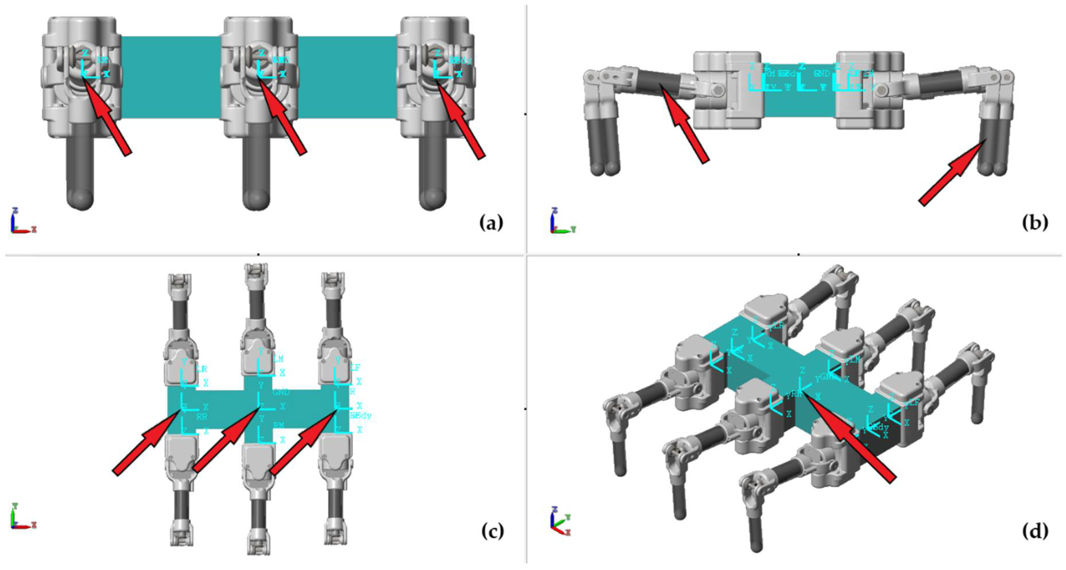
The pose (i.e., the number of DOFs) of a six-legged walking robot’s foot is determined by the number of joints of the leg. An arbitrary position of the foot in three-dimensional space requires three joints. By using additional joints, the orientation of the foot (or lower leg, depending on the kinematic design) can be defined.
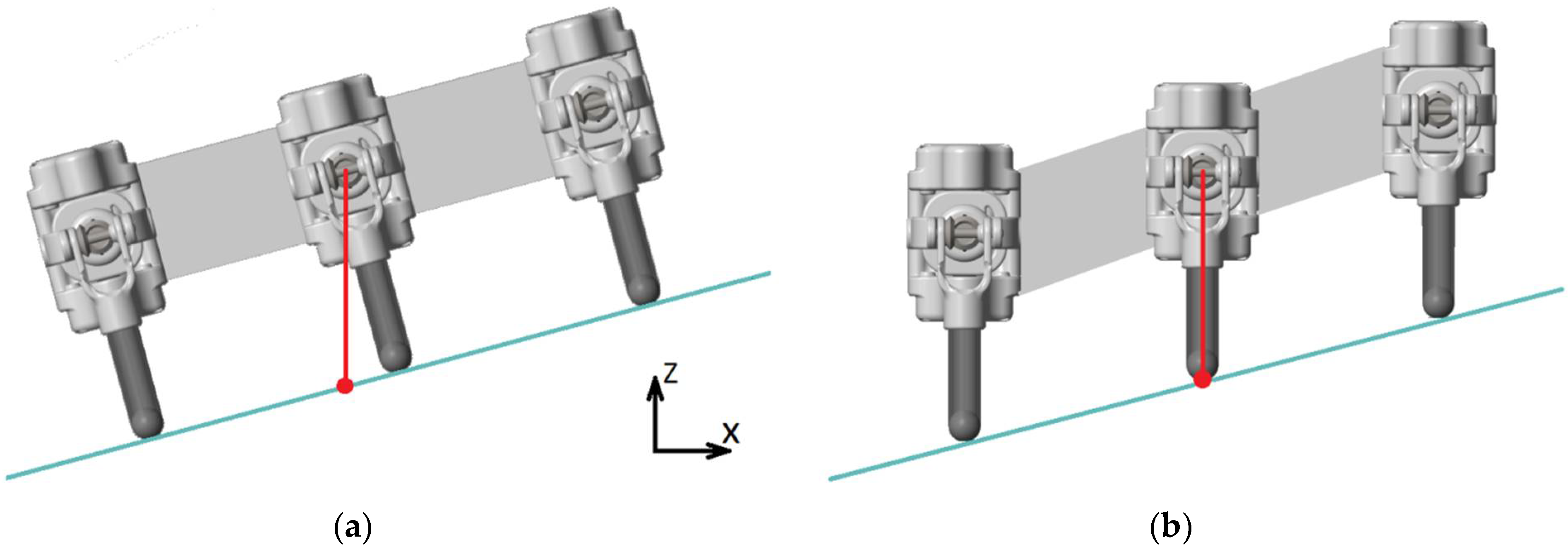
As a first step in the design of Szabad(ka)-III, the legs with three DOFs were implemented (see Figure 1a). The fourth DOF was added after the investigation of this solution (see Figure 1b). The main purposes of the implementation of the fourth DOF are both to allow the foot to rotate along the y-axis and to keep the foot motion in the yz-plane in case of sloping ground. The advantage of this is that the joints are less stressed, and the robot’s center of gravity is moved forward relative to the feet. With the introduction of an additional fifth joint (DOF), the longitudinal axis of the last leg segment (tibia or feet) can coincide with the vector of gravitational acceleration. A fifth DOF was not integrated as it would not be of significant benefit for Szabad(ka)-III due to the spherical design of the feet. It is important to note that, as the number of joints and the kinematic complexity increase, so does the mechanical inaccuracy of the robot since each joint has a certain amount of backlash. This phenomenon was also present in the case of the Szabad(ka)-II robot and was discussed in [19].
The Szabad(ka)-III robot was designed to have a modular structure. This means that the legs and body can be both changed and extended independently of each other. The motors in the leg module are responsible for moving three DOFs. The fourth DOF is implemented in the body module. If the only purpose of introducing the fourth DOF was to keep the leg vertical on sloping ground, then the rotation of six legs could have been achieved by a single actuator integrated in the body. However, the fourth DOF could also be used to make the robot’s front (or possibly rear) pair of legs act as a gripper. To achieve this, the fourth DOF should be moved leg by leg. The validity of this idea will be confirmed by subsequent simulations.
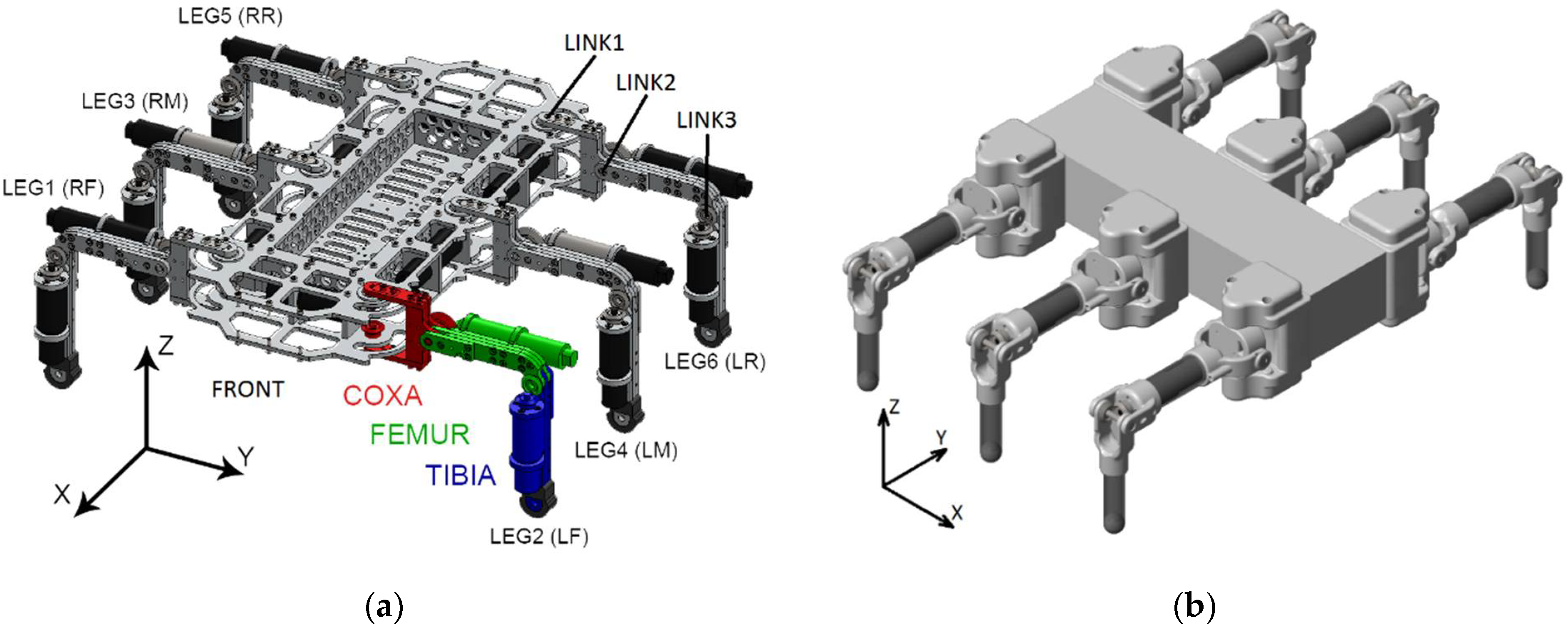
Compared to Szabad(ka)-II, the design of the new joints and the new leg structure of Szabad(ka)-III is much more advanced and sophisticated. A comparison between the two generations is shown in Figure 2.
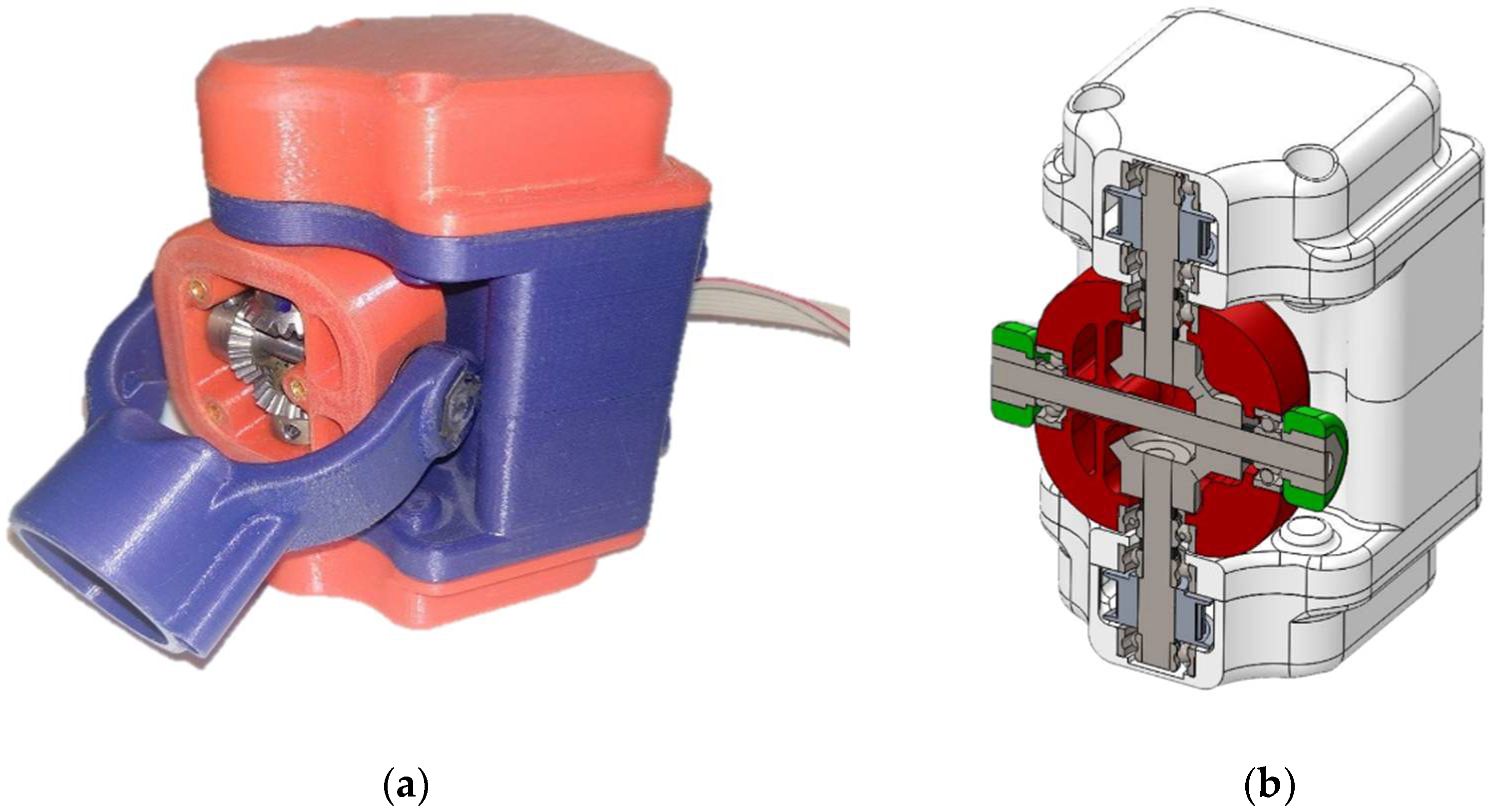
The leg is the most complex mechanical component of the robot. An integral part of the proposed leg is the novel differential gear drive system (see Figure 3). Using this solution, the torques of the two motors that originally moved link 1 and link 2 (as in Szabad(ka)-II) can now be used jointly to move the femur segment. Depending on the rotation speed of the two motors, the legs can be lifted or swung, or both movements can be performed simultaneously. During the swinging and lifting motions, both motors work together to achieve the desired movements. In the case of vertical leg motions, when the largest torques are applied, both motors lift the robot simultaneously. This solution results in less weight and energy consumption. By adding up the torques, in principle, motors with half the torque can be applied, allowing for all three motors to be of the same type. Another important feature of the leg is the triple spring-damper system in the tibia segment. Its function is to absorb the high-frequency vibrations that are generated when the foot touches the ground, minimize lower-frequency vibrations during walking and possibly recover the collected energy, and absorb large-scale forces in the event of a fall. The novel leg structure of the robot is described in detail in [28].
The body of the robot contains both the electronics and battery and can be fitted with the sensors that are to be implemented later (e.g., IMU, LIDAR, RGB/RGBD camera). Regarding the dimensions of the body, its length and the distance between the front and rear pairs of legs were predefined. An additional requirement was that the robot should be able to carry a payload of 2 kg.
The battery was selected based on the following criteria: maximum energy density, the weight of around 0.5 kg, and voltage greater than 12 volts (to power the 12-volt motors). Based on these requirements, a 14.8-volt, 5000-mAh capacity, 30C rating, 4S1P configuration LiPo battery with a weight of 550 g was chosen. At nominal values, such a battery can store 266.4 kJ of energy, and with the 30C discharge rating, it can provide 150 amperes of continuous current, which is significantly higher than the sum of the peak currents of the motors (see the current peak results in [19]).
The mechanical characteristics and properties of Szabad(ka)-III (compared to its predecessor) are listed in Table 1.
3. Szabad(ka)-III Robot Model
Both the development and operation of the Szabad(ka)-II robot model are described in detail in previous articles by the authors [1,19]. Article [1] details the mathematical foundations of the model, and article [19] describes the validated Simscape Multibody model of the robot. The model of Szabad(ka)-III was derived based on the methods and solutions introduced in [19], so the modelling process is not detailed here.
The mechanical elements of the model can be classified into two groups:
- -
- The pre-designed elements (the differential joint connecting the body and femur, and the joint between the femur and tibia);
- -
- Variable-parameter elements (the tibia and femur segments and the body itself).
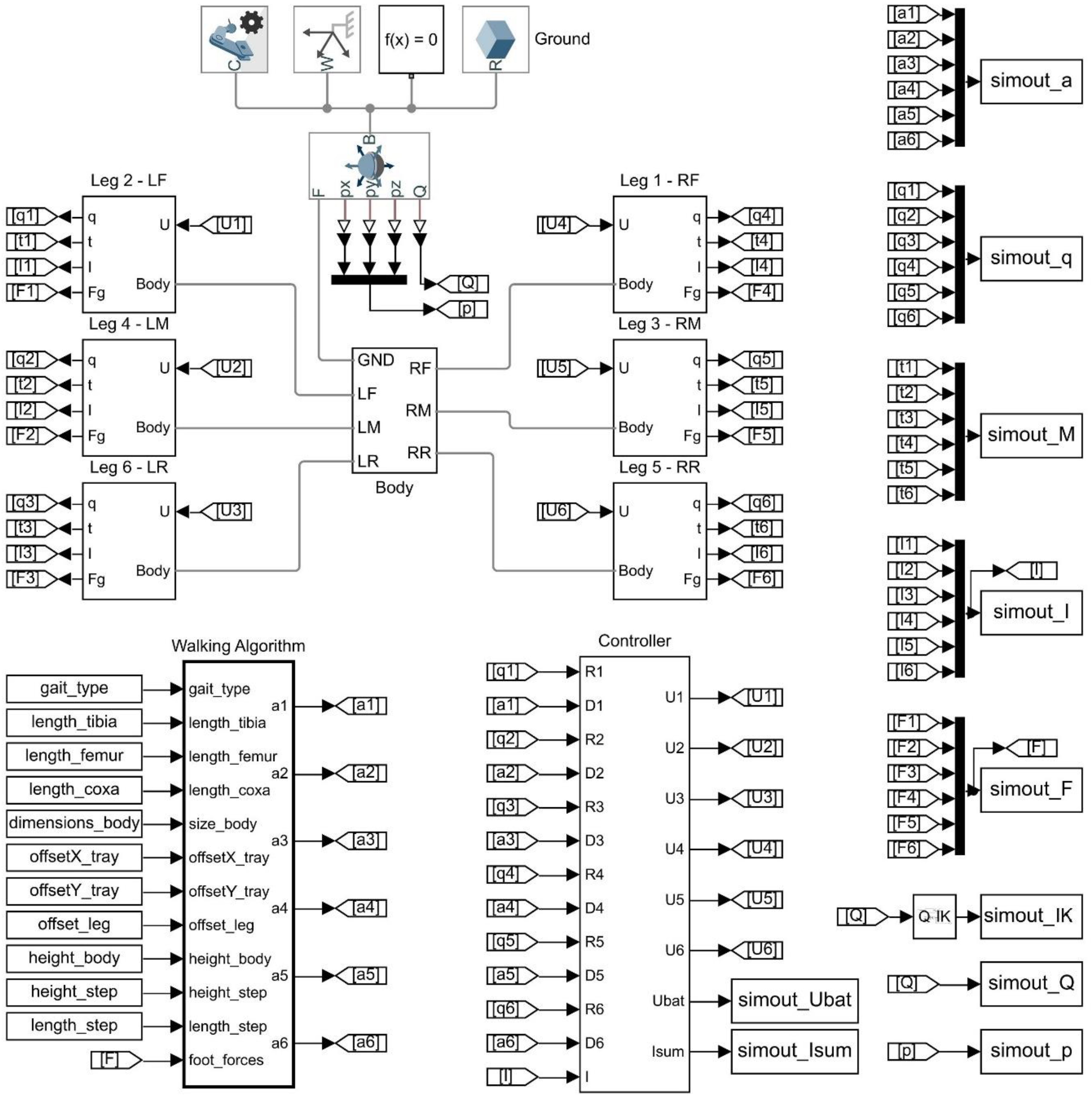
The elements of the first group, due to their complexity, had to be pre-designed in a separate CAD program (SolidWorks) and then imported into the robot model using Simscape Multibody Link. The elements of the second group, due to their simplicity, were designed directly in the Multibody model, which allows for easy parameter changes. The Multibody model of the robot is shown in Figure 4.
This modularly built robot model executes the robot’s equations of motion in a closed-form as (see Equation (1)):
where, in the case of joints (for Szabad(ka)-III, ), denotes the driving torques/forces ( dimensional matrix), indicates the wrist coordinates ( dimensional column vector), , is the inertia matrix ( dimensional), represents the Coriolis and centrifugal torques ( dimensional matrix), denotes the gravitational force ( dimensional column vector), is the dimensional vector of the external forces, is the number of effectors (for a hexapod, ), and is the dimensional Jacobian matrix of the robot effector. See the detailed derivation in [1,19].
In addition to the mechanical description of the system, the established Multibody model also includes a detailed mechatronic definition of both the motors and reductors. Furthermore, on the software side, the model includes the walking algorithm and the motor control subsystems.
The walking algorithm runs a MATLAB code at a frequency of 100 Hz to both determine the positions of the feet and perform the inverse kinematics calculations. The system can simulate three types of gaits (wave, ripple and tripod); moreover, it can be used to set the step length, height, and trajectory offset. The output is constituted by the angular positions of the motors.
The motor control subsystem includes a PID controller and the battery model. The PID controller part calculates the motor voltages based on the desired and actual joint positions. The battery model part determines the supply voltage based on the current drawn by the motors and the internal resistance of the battery.
Most of the relevant parameters of the model can be changed. The list of parameters is shown in Table 2.
The initial values of the parameters that can be varied by the optimization were determined based on the dimensions of the previous robot, and the limits allowed by the optimization were set so that the robot’s walking algorithm and inverse kinematics could implement all planned leg motions.
Some parameters are fixed, i.e., these parameters could not be tuned by the optimization algorithm. The length of the robot’s body (the distance between the two extreme coxa-coxa junctions) was a predefined condition. The dimensions and mass of the body electronics and the battery parameters were also predefined. The contact between the feet and the ground was not slippery, so the friction parameters of the feet were also constant. The friction in the joints was determined during the validation performed in the earlier work [19]. During the validation of the Szabad(ka)-II robot, the phenomena of gear backlash and reductor self-locking were also investigated. However, these phenomena were not considered in the modelling of the Szabad(ka)-III robot, as the improved mechanics (redesigned bearing and gear transmission of the wrists) eliminated the backlash, and the continuous motion (different walking algorithm) did not allow for self-locking of the reductors.
The list of the output variables generated by the simulations (some of which form the variables of the objective functions) is shown in Table 3.
During the validation of the Szabad(ka)-II robot, the mechanical structure was subjected to extreme stresses, resulting in high-frequency transients in the observed current curves. For this reason, the output variables in that problem were obtained with a higher sampling rate (500 Hz) [19]. In contrast, no high-frequency events occurred during the simulation for the structural optimization of the Szabad(ka)-III robot. Based on an analysis of both the initial signal curves and previous studies [1], the output variables of the simulation results were sampled at 100 Hz.
4. Formulating the Optimization Problem
To perform the optimization of electromechanical parameters, it is necessary, on the one hand, to have a properly functioning, preferably validated model and, on the other hand, to define the objective of the optimization, the parameters to be optimized and the optimization test environment (scenario).
The Szabad(ka)-III robot model is based on the validated model of its predecessor, Szabad(ka)-II [19]. The results of reference [19] enabled the incorporation of validated model parts (i.e., motors, reductors, and gear transmissions) in the derivation of the Szabad(ka)-III robot model. As a result, the established Szabad(ka)-III simulation environment is more suitable than a standard, motion-equation-based theoretical model, since the critical differences between simulation and reality are limited. The Szabad(ka)-III robot model-based optimization constitutes a realistic framework, which facilitates the design, manufacturing and assembly of real hexapod mechatronics systems.
The following subsections present the definition of the optimization objectives, parameters, test environment and the rationalization of the number of parameters.
4.1. Optimization Objectives (Fitness Function)
The aim of the optimization of the Szabad(ka)-III robot model is to select the appropriate electromechanical elements and create the ideal mechanical structure. The purpose of the fitness function (also called the utility function, cost function or loss function) is to properly aggregate the different goals (preferences), i.e., to add up the defined objectives with appropriate weights, so that the optimization can find the global minimum based on a scalar fitness rating. However, neither the definition of the objectives nor the compilation of the fitness function is a straightforward task for a complex robot structure, as the optimization can have many hard-to-define goals and interrelated parameters.
- -
- Minimizing energy consumption,
- -
- Minimizing mass,
- -
- Maximizing speed and dexterity,
- -
- Minimizing unwanted body motion,
- -
- Minimizing adverse effects on the structure, and
- -
- Minimizing differences between joint torques.
Minimizing energy consumption is generally an important condition when increasing both the operating time and distance travelled for a given battery. This can easily be determined by measuring the amount of energy that is required for the robot to travel a given distance. The objective function of the energy consumption can be described by the following formula (Equation (2)):
where is the objective function of the energy consumption, is the energy used to travel the distance, is the distance travelled by the robot, is the battery voltage, is the total current of the motors and is the time required to travel the distance.
A common performance metric used to compare the energy efficiency of walking robots is the cost of transport (CoT) (Equation (3)) [29,30]:
where is the robot mass and denotes the gravitational acceleration.
If the mass of the robot does not change during the optimization, then the term is constant and does not play a role in the comparison of energy consumption. Thus, the objective function is appropriate for minimizing energy consumption.
In [29], CoT is used to compare different control algorithms on the Weaver hexapod robot, and in [30], CoT is used to compare the MIT Cheetah quadruped robot with other robots and biological runners.
The aim of minimizing mass is also to increase the running time and distance travelled. In terms of the simulation, the robot is composed of fixed and variable mass elements. The constant mass elements are the robot’s electronics (drives, battery) and the pre-designed joints (joint housing, motor-reductor units). The variable mass elements are the tibia and femur segments and the body itself. The mass objective function can be described by the following formula (Equation (4)):
where is the objective function of the mass, and denote the mass of the robot’s components.
The robot’s speed and dexterity depend on the area that the foot trajectory can cover, i.e., how far the robot can step. Typically, and in the case at hand, speed and dexterity are not optimization objectives to be maximized, but predefined parameters. The optimization process has to consider whether the inverse kinematics of the robot model can meet the expectations of the given parameters. If the expected foot position cannot be obtained, the objective function must return a penalty. The objective function for dexterity can be described by the following formula (Equation (5)):
where is the objective function of the dexterity, is the penalty value, and is the return value of the model that shows whether the executed sequence of steps was successful.
An unwanted motion of the body, i.e., any translational or rotational motion of the body other than the expected direction of travel, in other words, a wobble or shake in the robot, clearly interferes with the operation of the sensors (e.g., camera, LIDAR, IMU) and the parasitic movements increase energy consumption. Therefore, minimizing this phenomenon is also a fundamental task. Since the main concern in sensor measurements is the elimination of extreme events, the RMS of the unwanted motion along the largest axis is considered. The objective functions for translational motion (Equation (6)) and rotational motion (Equation (7)) can be described by the following formulas:
where denotes the translational error in the x-direction, denotes the translational error in the y-direction, denotes the translational error in the z-direction, denotes the rotational error along the x-axis, denotes the rotational error along the y-axis, denotes the rotational error along the z-axis, and denotes the length of the simulation .
The adverse effects on the structure are mainly understood as vibrations and parasitic torques in the mechanically and electronically sensitive parts of the robot. The importance of minimizing these harmful phenomena depends on the expected lifetime of the robot and its reliability. They also increase energy consumption, especially when an aggressive controller is used.
One example of the condition monitoring of industrial robots is shown in [31]. Vibrations in industrial robots are generated by the moving parts of the machine, and high-amplitude vibrations are often considered a predictor of future failures. However, vibration analysis should also be performed for mobile robots to optimize the design or operation of the robot. An example of this can be seen in [32], where a vibration analysis of a crawler-type inspection robot was performed to optimize its travel speed.
Based on the design of the Szabad(ka)-III robot, vibrations can be investigated at three locations: tibia–femur joints, femur–coxa joints, and the body. The vibrations in the joints can damage the reductors, gears and bearings, while the vibrations in the body can damage the electronics. The distinction between upper and lower joints is also useful because the differential mechanism in the upper joint is, by design, more sensitive than that in the lower joint.
To quantify vibration magnitudes, the peak or RMS of the translational or rotational velocity or acceleration spectrum could be used. In the case of walking robots, it is worth considering the highest of the three axis vibration magnitudes (see the detailed derivation in [33]).
On this basis, the objective function of the vibrations occurring in the body of the robot can be described by the following two equations (Equations (8) and (9)):
In Equations (8) and (9) , and are the spectrums of translational or rotational velocities or accelerations of the robot body in the x, y and z directions as a function of frequency , respectively. The determination of these components is discussed in [33].
In addition to optimizing the electromechanical characteristics of the robot, the aim may also be to reduce manufacturing costs or complexity. One way to do this is to unify certain components (e.g., use the same motors and reductors). The use of the same motor-reductor units on the robot can be achieved by minimizing the differences between joint torques.
By default, different joints in a robot have significantly different torques. A good example of this is the previous robot, Szabad(ka)-II, which had large torque differences due to both the tripod walking algorithm and its legs being arranged in a line on each side; thus, three different motor-reductor units were employed in the mechanics. This significantly complicated the design and increased the robot’s production costs.
However, in the case of Szabad(ka)-III, it is worth considering normalizing the torques in the joints to enable the use of identical motor-reductor units. This can be carried out in two ways during optimization. One is to determine the maximum acceptable torque values in the joints and to penalize values above this in an objective function. The other solution is to measure the difference between the torques and minimize it. The difference is expressed as the standard deviation between the RMS values calculated for the joint torques , since smaller deviation means that values are closer to each other, regardless of the mean value. The RMS function represents the magnitude of the torque by quadratic averaging, which means that larger values are more easily considered than smaller values compared to the simple average calculation. Based on these, the objective function of the torque differences can be described by the following formula (Equation (10)):
where is the number of joints (for Szabad(ka)-III, K = 18), is the torque measured at joint and is the RMS value calculated for the torque measured at joint .
An example of the unification of the elements driving the joints can be seen in the case of the SpaceClimber hexapod robot. Here, the aim was not to reduce costs: to simplify space qualification procedures in further steps, all 24 actuators driving the legs were built identically [11].
The objective functions used to optimize the robot structure are summarized in Table 4.
The fitness function can be derived by adding the partial objective functions and weighting them accordingly. If all objectives are considered, then the following formula is obtained (Equation (11)):
where is the objective function of energy consumption, is the objective function of mass, is the objective function of dexterity, is the objective function of translational motion, is the objective function of rotational motion, is the objective function for vibrations, is the objective function for the differences between joint torques, and , , , , , , and constants weight the preferences.
4.2. Optimization Parameters
Previous research has determined that a robot should be six-legged, which is an ideal ratio of stability, redundancy and speed of travel [1]. In addition, hexapods have a certain level of mechanical fault tolerance, i.e., they are able to walk with a failed leg using a suitable fault-tolerant walking algorithm and adaptive gait planning [34,35].
Three structural concepts can be distinguished on the basis of the leg arrangement:
- -
- Axisymmetric;
- -
- Symmetrical only along the longitudinal axis;
- -
- Symmetrical along the longitudinal and lateral axes.
An axisymmetric layout is recommended for robots with omnidirectional walking. This gait was not an important consideration for Szabad(ka)-III, so this solution was discarded. The robot should be optimized for straight walking with the possibility of turning. The question of whether there is an advantage to the longitudinal only symmetry, which is also common in the insect world, remained. Whether, and to what extent asymmetry between the front and the back of the robot is necessary, can also be decided by optimization. One of the goals of double asymmetry could be to deal with the phenomenon of rearing [1] or climbing on sloping ground or stairs.
The parameters to be optimized can be divided into three major groups. These are the structural, spring-damper and walking algorithm parameters.
The parameters of the geometric structure can be divided into the following subgroups:
- -
- Leg segment length: This includes the length of the tibia and femur. For Szabad(ka)-III, the coxa has zero length due to the differential joint, and a separate tarsus segment is not present due to the design of the foot. The tibia and femur (whose lengths are interpreted between the rotational axes of the joints) are shown in Figure 5b.
- -
- -
- Positioning of the center of gravity in the body: The center of gravity of the electronics and the battery can be moved inside the body along the x- and z-axis relative to the center of the robot (Figure 5d).
- -
- Choice of motors and reductors: Unlike before, these two parameters are not continuous but can take discrete values, i.e., it is possible to choose which of a given manufacturer’s products can deliver the appropriate torques.
The robot is designed to be symmetrical along its longitudinal axis, so the length of the leg segments and the positioning of the legs are defined per pair of legs (front, middle and rear leg pairs).
The spring-damper system of the legs has the following parameters:
- -
- Spring constant and damping coefficient of the feet: The main function of the triple spring-damper system in the tibia segment is to absorb vibrations during walking. The triple spring-damper system is described in detail in [28]. Therefore, the optimization involves the determination of three spring constants and three damping coefficient parameters.
The parameters of the walking algorithm can be divided into the following subgroups:
- -
- Posture: This includes the height of the body above the ground (other posture parameters should be taken into account when optimizing the walking algorithm).
- -
- Foot trajectory: This includes the height and the length of the trajectory (same for all feet), its offset in the direction of travel and its distance from the body (per pair of feet).
The optimization parameters are summarized in Table 5.
4.3. Reducing the Number of Parameters
The difficulty of the task is increased by the large number of parameters to be optimized and their interactions. On the one hand, many parameters increase the optimization time; on the other hand, most of the parameters are interrelated and changing them separately may lead to similar results. For example:
- -
- If the goal is to achieve a given speed (step length), the same result can be achieved by changing the position of the legs, the length of the segments, or the length of the trajectory.
- -
- If the goal is to achieve sufficiently low joint torques for a given mass, this will be influenced by the torque of the motors, the positioning of the legs, the length of the segments, and the posture.
As a result, many local minima can be generated during the optimization process. Whether different varying parameters will lead to similar effects can be determined with higher probability by examining the number of local minima.
For these reasons, it is worth considering the following options:
- -
- The number of parameters can be reduced if it is likely to be unnecessary to optimize all of them.
- -
- If the same result can be achieved by modifying several different parameters, than the parameters that are more expedient to determine based on the production conditions can be taken out of the optimization.
- -
- The optimization can be broken down into a number of sub-optimizations if the appropriate objectives and the associated parameters that influence them the most can be categorized.
As defined in the previous chapter (Table 5), 17 structural, six spring-damper and nine walking algorithm parameters, for a total of 32 parameters, need to be defined. This is a very large number that should be reduced before starting the optimization.
4.3.1. Investigating the Reduction in the Number of Structural Parameters
The length of the tibia and femur, the X and Z position of the coxa and the Y distance between the legs are determined for each pair of legs. For the three pairs of legs (front, middle and rear), this leads to 3 × 5 parameters. However, if the robot is also symmetric along its lateral axis, then only two pairs of legs (outer and inner) are required, resulting in 2 × 5 parameters. In addition, it is not necessary to separately define the connection positions of the inner and outer coxa segments. It is sufficient to change only the position of the inner in relation to the center of the outer. The combined height of the pairs of legs would affect the center of gravity of the body, but this can be adjusted separately.
4.3.2. Investigating the Reduction in the Number of Spring-Damper Parameters
There are three springs in the robot leg. Moving from the foot, the first is the rubber coating of the foot, whose function is to absorb the high-frequency vibrations generated when the leg touches the ground; the second is a softer steel spring, to minimize the lower-frequency vibrations during walking and possibly restore the gathered energy; the third is a harder steel spring to absorb the large-scale forces in case of falling. The optimization carried out at present does not consider the robot’s fall and neglects the effect of the thin rubber coating of the feet; therefore, one spring constant and one damping coefficient parameter should be considered.
4.3.3. Investigating the Reduction in the Number of Walking Algorithm Parameters
Since there are two sets of pairs of legs instead of three, shifting the trajectory in the X and Y directions will result in 2 × 2 parameters instead of 3 × 2 in this case, too.
The parameters that remain after rationally reducing the number of parameters are summarized in Table 6.
The number of parameters to be optimized is reduced from 32 to 19 based on the aforementioned concepts.
4.4. Optimization Scenarios
To perform the optimization, the appropriate test environment must also be defined. For Szabad(ka)-III, the following factors had to be defined:
- -
- The robot’s walking velocity;
- -
- The terrain characteristics;
- -
- The selected walking algorithm.
It is recommended to run the simulation at a walking velocity that will be both frequently used in practice and sufficiently high to manifest the physical phenomena of extreme stress. Therefore, the highest speed at which the robot can follow the trajectory of the foot without any error (deformation) has been chosen.
The terrain characteristics include the following:
- -
- Ground slip (friction between the ground and the foot);
- -
- Ground slope (the angle between the horizontal and the ground plane);
- -
- The nature and size of obstacles on the ground.
The analysis of the Coulomb friction between the ground and the foot is described in detail in [19], where the friction coefficient has been determined experimentally. The foot of Szabad(ka)-II robot was covered with a rubber coating and no slippage occurred during practical measurements while walking on straight ground. For Szabad(ka)-III, we plan to use a similar rubber feet coating, and, therefore, the phenomenon of slippage is not considered. The Coulomb friction coefficient is set to µ = 1, which corresponds to the friction between dry rubber and concrete. For walking on special, slippery ground, the simulation can be extended by varying the friction coefficient.
Compensation and handling of the ground slope is the task of the fourth leg joint. The fourth joint is used to ensure that (from the side view) the legs are not perpendicular to the ground, but that their axis coincides with the vector of gravitational acceleration. In this way, the robot’s center of gravity is also moved forward when travelling uphill, which significantly reduces the chance of its tipping over (falling backward). The Szabad(ka)-III robot is designed to walk on sloping ground (its legs are also designed with four DOFs). Optimization must be performed on both straight and sloping ground. Accordingly, three optimization environments have been defined: straight ground, the slope of 30 degrees inclination, and the slope of −30 degrees inclination.
The structural optimization was performed on even ground with no obstacles. The reason for this is that, by varying the segment dimensions, the legs would randomly collide with the obstacles, and this would lead to stochastic results. A test environment with obstacles will be applied to the optimization of the walking algorithm in the forthcoming research.
The most commonly used gaits for the choice of the walking algorithm are Wave, Ripple, and Tripod gait. These gaits are characterized as follows.
- -
- Wave gait is the slowest gait, with five feet on the ground and one foot in the air at a time.
- -
- The ripple gait is a medium-speed gait with four feet on the ground and two feet in the air at a time.
- -
- The tripod gait is the fastest gait, with three feet on the ground and three feet in the air [36].
In the case of the tripod gait, the two outer feet are simultaneously on the ground on one side of the robot and the inner feet on the other side. As a result, the middle leg experiences nearly twice the load of the outer legs. For the validation of Szabad(ka)-II, this gait was used, as the aim was to put extreme stress on the structure. As a result, stronger motor-reductor units had to be built into the middle legs.
However, for the optimization of Szabad(ka)-III, the intermediate option was chosen, i.e., the ripple gait, where two legs are on the ground on each side at the same time, so that the load on the legs is uniform. The resulting structure is, by default, not ideal for a tripod gait, but this problem can be solved by a separate optimization of the gait parameters later, including a Y-directional shift in the foot trajectory.
5. Optimization
5.1. Search Method
The optimization was performed using a Particle Swarm Optimization (PSO) heuristic search algorithm. The process was developed based on previously acquired and published experience (see [19,22,37]). In the sequel, the process of selecting the appropriate fitness function was first described, and then the novel multi-step optimization process was introduced.
5.2. Fitness Function
The objectives of the optimization were to minimize energy consumption, maintain speed and dexterity, minimize unwanted body motion and minimize differences between joint torques.
To minimize unwanted body motion, the rotational motion was minimized based on the nature of the sensors mounted on the robot body (this is because, for example, a few degrees of rotation on a camera will result in a much larger error than a few millimeters of displacement). Minimizing the differences between joint torques should be ensured for joints that are subjected to higher loads. In the case of Szabad(ka)-III, the two motors of the differential gear drive had higher loads, and their torques were, therefore, minimized. The joint moving the tibia was subjected to lower loads and, therefore, its torques did not need to be changed.
When setting the weight parameters of the fitness function, the goal was to ensure that the objectives were equally considered and therefore normalized. In other words, the weights of the objectives were chosen so that the original objective values obtained with the initial structural parameters would have a value of 1 after normalization. The exception to this is the penalty function of the dexterity, which returns a value of zero when walking without error and a larger value when walking with error. The fitness function can be described by the following formula (Equation (12)).
The final multi-scenario fitness function is the weighted sum of the fitness functions run over the three scenarios. Since the importance of walking on the straight ground is greater, the weight for this scenario is set to 2, and the weight for the other scenarios is set to 1. Based on these, the multi-scenario fitness function can be described by the following formula (Equation (13)):
Based on the above, the fitness value of the simulation with the initial structural parameters determined by technical considerations is , and the multi-scenario fitness value is . The improvements in the results can be compared to this value.
5.3. Multi-Step Optimization
In the first attempts of the optimization procedure, all 19 parameters were optimized simultaneously. However, after running the optimization several times, it was noticed that, although the resulting fitness values were similarly low, the parameters varied too much. This is clearly shown in the “All Parameters” column of Table 7. This suggests that the optimization algorithm ran into local minima. The reason for this could be the high number or redundant nature of the parameters, as mentioned earlier.
This phenomenon can be mitigated by further reducing the number of parameters or by adding more objectives to the fitness function. However, these would be artificial changes that would conflict with the original goals. Additionally, a larger population search would have improved the results, but running the dynamic model simulation is particularly time-consuming due to the high level of detail of the model. On the six-core Intel Core i7-8700 computer, used in the optimization, the running time for one iteration was about 55 min. A 500-iteration optimization takes 4–5 days. Therefore, the aim was to develop a solution that would produce the best possible results with a low number of iterations.
Based on the above, a novel approach of grouping (classifying) the optimization parameters and performing the optimization in multiple steps was chosen. However, this required the basis for grouping to be determined. It makes sense to optimize the “more important” parameters first, but the question is which parameters are considered important. To determine this, the convergence rate (CR) introduced in [22] can be used. The CR shows how much the parameter converges towards the optimum during the optimization as a function of the fitness value. In other words, this refers to the importance of the parameter in achieving the estimated optimum [22]. The CR values of the parameters were determined by the previously performed 19-parameter-based optimizations. An examination of the data also revealed that the variance in the parameters obtained as a result of the optimization is correlated with the CR values. Parameters with a higher variance typically had lower CR values. This also indicates the suitability of using the convergence rate.
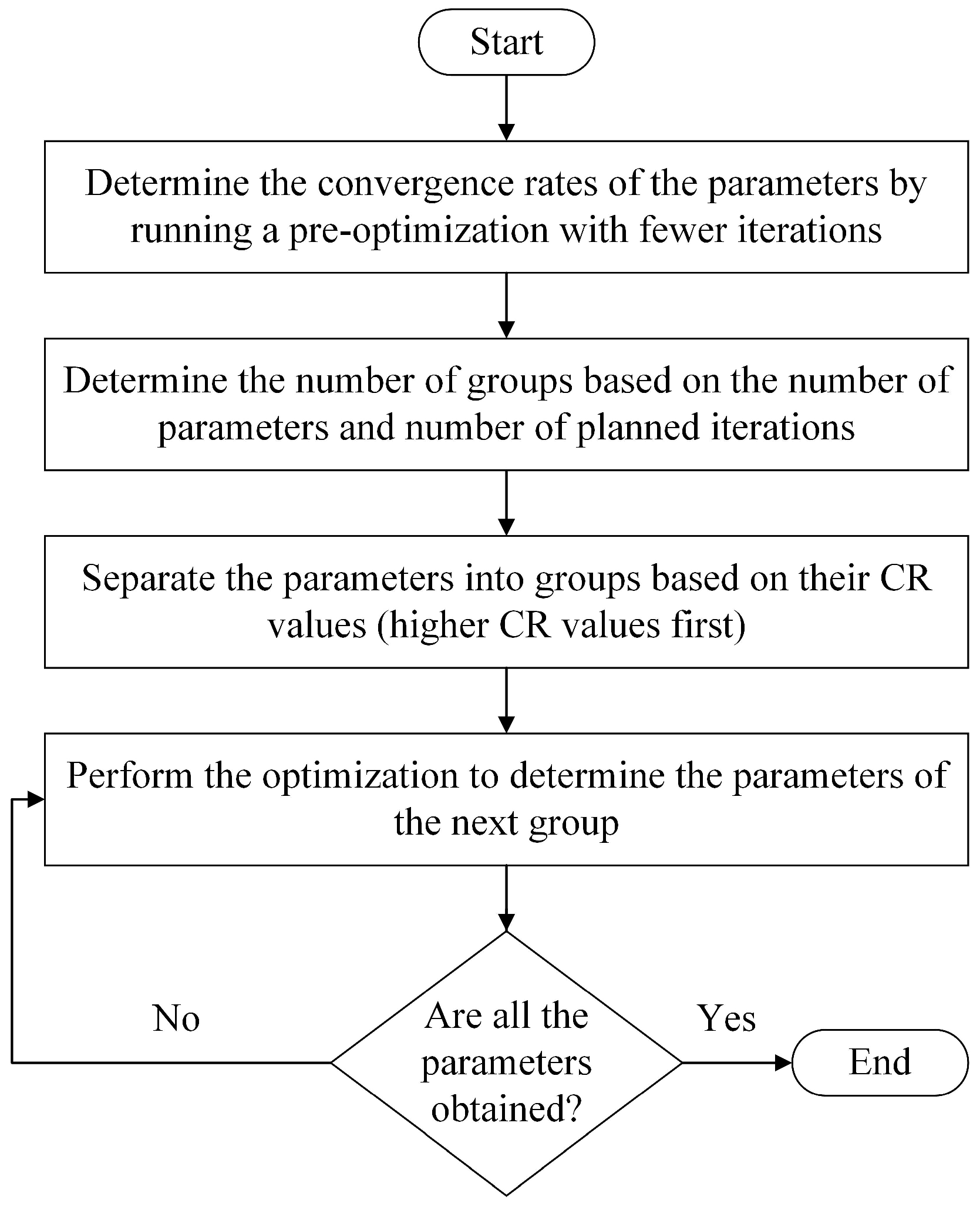
The flow chart of the multi-step optimization based on the parameter importance and grouping is shown in Figure 6.
5.4. Optimization Results
Based on the above, the structural optimization of the robot was divided into two steps. In the first step, the optimization of the parameters with the 10 highest CR values was performed. The other parameters were left at their initial values. To check the variance in the results and the appropriate depth of the search, the optimization was also performed with two different population and generation numbers (i.e., 80 × 30 and 120 × 40 searches were executed). The results are shown in the “First Step” column of Table 7. The resulting parameters showed very similar values for both the lower and the higher depth optimization. An exception is the body height parameter, but this also had a lower CR value, so it can be assumed that it indeed has less impact on the fitness function. The fitness results already show similar values as for the 19-parameter-based optimizations.
The second step, using the parameters obtained in the first step, optimized the remaining nine parameters and two parameters carried over from this first step (body height and inner leg trajectory offset in the Y-direction).
The value of the body height was also included in the parameters of the second step because of the variance shown in the first step and its otherwise important function. The inner leg trajectory offset in Y direction was optimized once again because this parameter received the highest CR value and because this parameter affects the characteristic elliptical arrangement of the robot’s feet. It seemed worth checking whether the previous values would remain after the second step.
The optimization of the second step was also performed with two different population and generation numbers (i.e., 80 × 30 and 120 × 40 setups were executed). The results are shown in the “Second Step” column of Table 7. The variance in the resulting parameters was again very low, in this case, including the body height parameter. The fitness results show a significantly better performance compared to the 19-parameter-based optimization outcome.
Summarizing the results of the two-step optimization, the following can be concluded: by separating the parameters, the variance of the results was much lower than that in the case of the 19-parameter-based optimization. This suggests that the optimization avoided the local minima and that the selected population and generation number were appropriate. The first step has already shown similar fitness results to the output of the 19-parameter-based optimization; the obtained results were further improved in the second optimization step.
The objective results obtained by the two-step optimization (compared to the initial values) are shown in Table 8.
The changes achieved during the process led to significant improvements in the robot’s performance. An important practical aspect is a change in the robot’s range when walking on the straight ground, which is the most common application. With a single charge, using the battery storing 266.4 kJ of energy, before optimization, the robot had an energy consumption of 2881 J/m and was able to cover a distance of 92 m, and after optimization, it had an energy consumption of 2258 J/m and was able to cover a distance of 118 m. The significantly reduced rotational motion (shaking) results in a great improvement in the measurement of the sensors placed on the robot. By minimizing the differences in torque, the motors are subjected to lower than the allowed loads.
In the future, if an objective becomes a higher priority than the others, for example, if reducing energy consumption becomes more important than reducing vibration, the results can be further improved by adjusting the appropriate weight parameters of the selected objective.
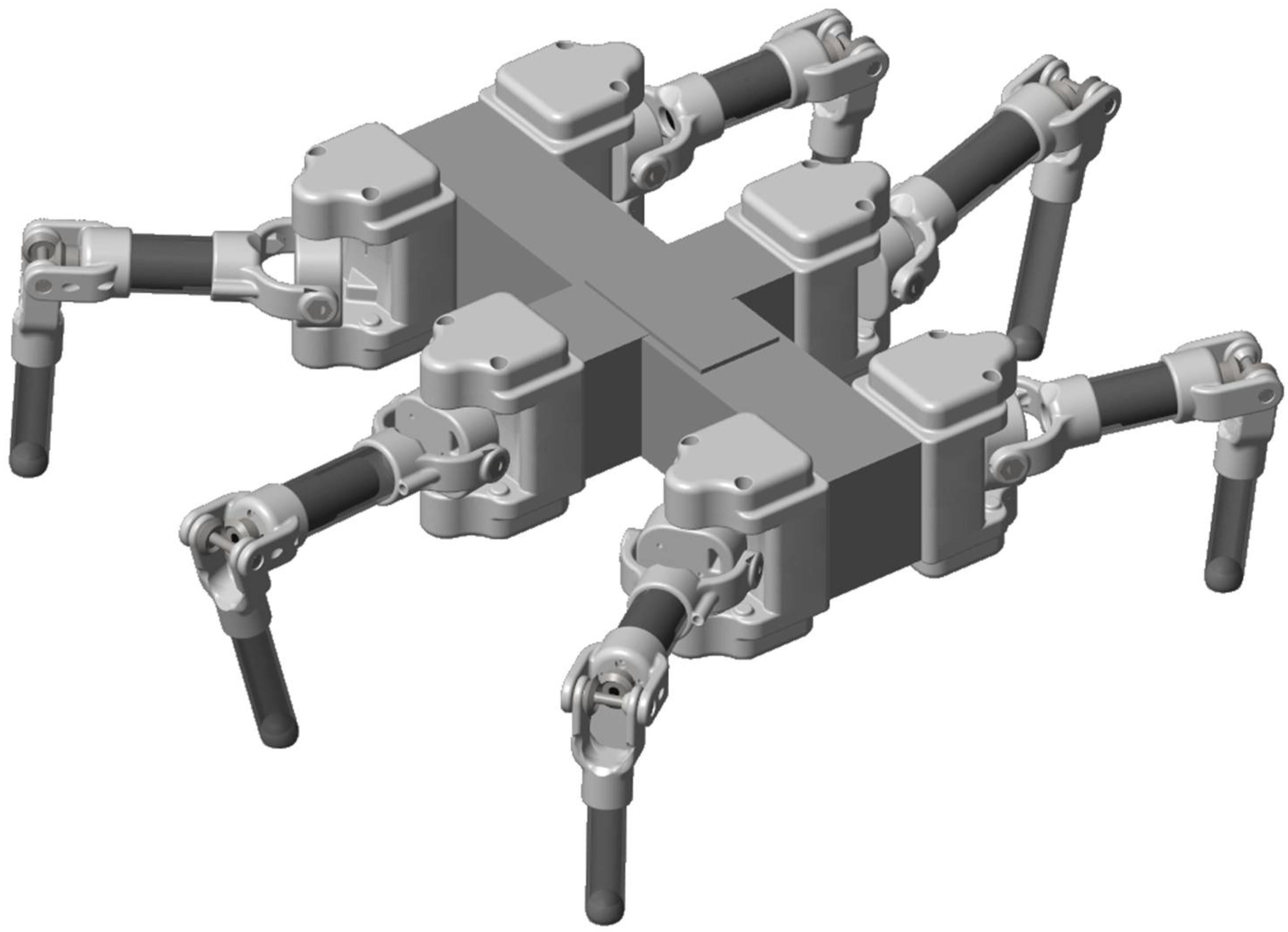
The new robot structure is shown in Figure 7.
The following logical conclusions can be drawn from the numerical data and figures:
- -
- The connection points of the inner legs along the y-axis are further away from the body, and those of the outer legs are closer. This more uniform distribution around the robot’s center of gravity increases its stability.
- -
- The trajectories of the outer feet have moved away from the center of the body along the direction of travel (x-axis), while the trajectories of the inner feet have changed minimally. This allows for the robot to take longer steps, and the feet in contact with the ground can cover more surface area, which also improves stability.
- -
- The length of the trajectory is close to the maximum allowed, which determines the size of the step. Larger steps reduce energy consumption.
- -
- The spring constant of the foot is also close to the maximum value. This may result in high-frequency vibrations; however, it may significantly reduce the low-frequency and high-amplitude wobbling of the body.
- -
- The center of gravity of the electronics has not changed much from its original central position. This helps to achieve a uniform distribution of mass around the geometric center of the body (this is the point at which the rotational movement of the body is measured).
5.5. Verification of the Optimization on Independent Scenarios
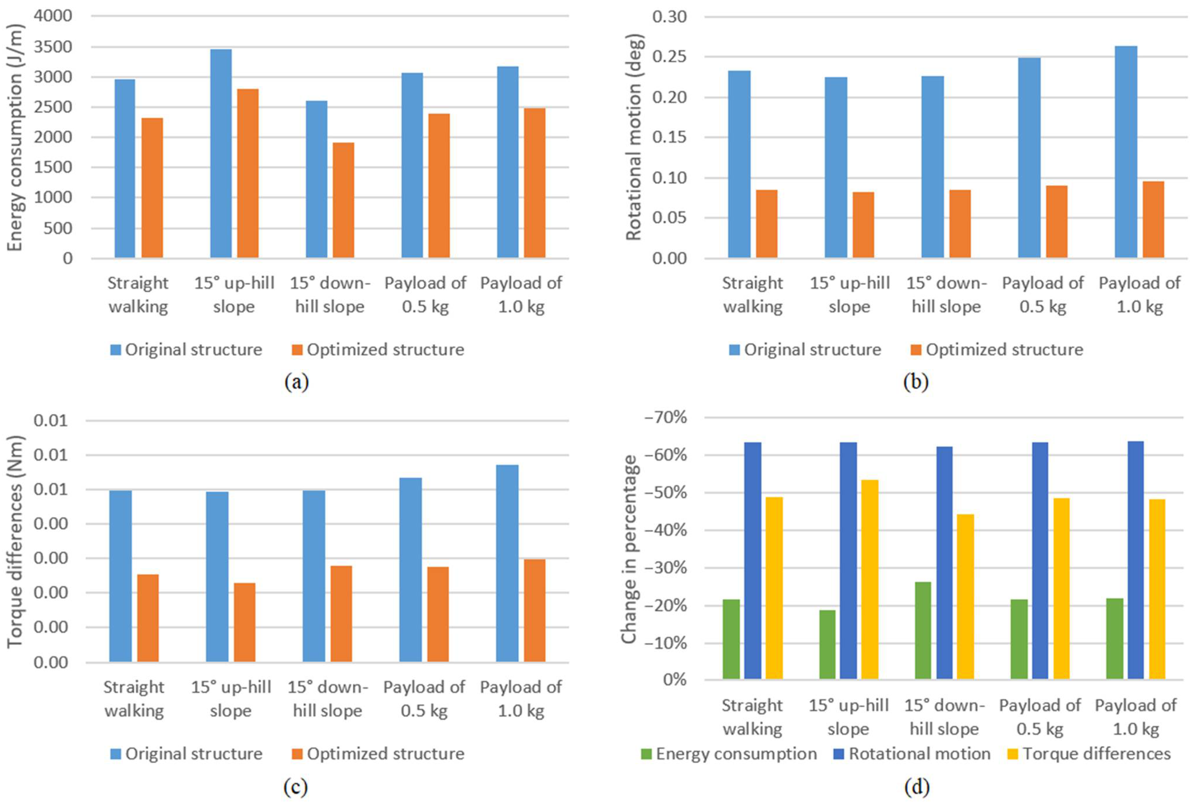
In order to verify the generality and robustness of the optimization procedure, the obtained structural parameters were evaluated in four independent simulation scenarios. Namely, walking on both 15-degree uphill and 15-degree downhill slopes was investigated; moreover, the effects of payloads of both 0.5 and 1.0 kg were also tested with the optimal parameters.
Figure 8 highlights the performance results in each scenario, where, for clearer comparison, the objective function values were not normalized.
The results of the objective functions significantly improved for all scenarios; they showed a similar outcome to the multi-scenario optimization (see Table 8). These results verify the generality of the obtained structural parameters.
The results related to energy consumption showed a slightly greater improvement in the downhill slope, where less energy is required for walking, and the results related to torque differences indicated a slightly better result for the uphill slope, where higher loads occur. The quality of rotational motion is even more similar in all cases.
These results conclude that the parameters obtained by the optimization process contribute to a generally improved structural robot design.
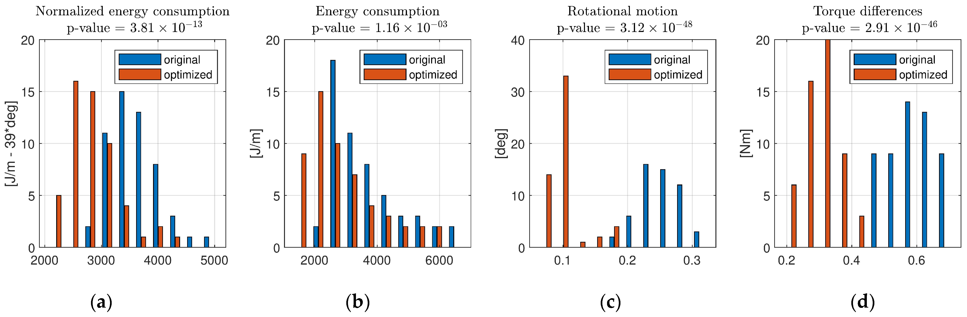
In order to show the significance of the proposed strategy, a statistical paired t-test was also applied for the analysis of the results before and after optimization. The simulations were run on 54 different scenarios with different slopes and payloads. The slopes ranged from −40 to 40 degrees in 10-degree increments (9 cases), while the payloads ranged from 0 to 2.5 kg in 0.5 kg increments (six cases). The variations of these cases resulted in 54 different scenarios.
The available set of objectives from the various scenarios (see Figure 9) approximates normal distribution, and the optimum structure (red) shows significant improvements compared to the original structure (blue); this is also confirmed by the t-test (p-value < 10−12 for each objective).
In order to make a correct statistical comparison, the Energy objective was linearly normalized by the angle: , to remove the direct influence of ground slope and energy consumption.
6. Conclusions
In this paper, a novel optimization method was presented, which forms the basis of the construction of the next generation of the Szabad(ka) robots, i.e., the Szabad(ka)-III robot. For the development of this method, a detailed dynamic model was used based on the results of the validated Szabad(ka)-II robot model.
The paper conducted an in-depth analysis of the objectives, parameters, and test environments of structural optimization. The objectives of the optimization of Szabad(ka)-III were to minimize energy consumption, unwanted body motion and differences between joint torques, while maintaining speed and dexterity. The process determined the parameters of the robot’s geometric structure, spring-damper system, and walking algorithm. Three scenarios were selected as the test environments: straight ground, 30-degree uphill slope, and 30-degree downhill slope. For each scenario, a non-slip foot contact, obstacle-free ground, and ripple gait were used.
The optimization procedure developed for problems with a higher number of parameters is designed to produce good results even with a small number of iterations. The procedure is based on the grouping of the optimization parameters and the implementation of the optimization in multiple steps, where the parameters are grouped according to their contributing factor. The contributing factor is estimated on the basis of the convergence rate introduced in [22].
As a result of the optimization, the values of energy consumption objective function, rotational motion objective function, and torque differences’ objective function were reduced by 22.16, 61.83, and 49.13 percent, respectively. Consequently, the robot’s range was significantly increased, and the vibration that negatively affects the sensor readings was reduced, while the motors were subjected to loads below the permitted values.
With the developed procedures, the optimization can be easily repeated if the expected parameters (e.g., payload or enclosing dimensions of the robot) or scenarios (e.g., walking algorithm, ground slip) change. Thanks to the modular leg and body design, the physical robot can be relatively easily modified according to the new results.
After the optimization is successfully performed, the next step in the development process is to physically build the robot and verify the chosen morphology. Further steps in the research will focus on the minimization of adverse effects on the structure and the forces to which the robot will be exposed in case of a fall. Another future goal is to optimize the robot’s walking parameters using different walking algorithms and walking speeds to further minimize both energy consumption and vibrations.
Author Contributions
Conceptualization, E.B. and P.O.; methodology, E.B. and P.O.; software, E.B.; validation, E.B., Á.O. and I.K.; formal analysis, E.B. and J.A.; investigation, E.B. and P.O.; resources, E.B. and P.O.; data curation, E.B.; writing—original draft preparation, E.B.; writing—review and editing, E.B. and Á.O.; visualization, E.B.; supervision, P.O.; project administration, P.O.; funding acquisition, P.O. All authors have read and agreed to the published version of the manuscript.
Funding
This research was funded by the 2020-1.1.2-PIACI-KFI-2020-00173 project. The project is co-financed by the European Union.
Institutional Review Board Statement
Not applicable.
Informed Consent Statement
Not applicable.
Data Availability Statement
Not applicable.
Conflicts of Interest
The authors declare no conflict of interest.
References
- Kecskés, I.; Burkus, E.; Bazsó, F.; Odry, P. Model validation of a hexapod walker robot. Robotica 2015, 35, 419–462. [Google Scholar] [CrossRef]
- Silva, M.F.; Machado, J.A.T. A literature review on the optimization of legged robots. J. Vib. Control 2011, 18, 1753–1767. [Google Scholar] [CrossRef]
- Ding, X.; Yang, F. Study on hexapod robot manipulation using legs. Robotica 2016, 34, 468–481. [Google Scholar] [CrossRef]
- Grzelczyk, D.; Stańczy, B.; Awrejcewicz, J. Power consumption analysis of different hexapod robot gaits. In Proceedings of the 13th International Conference on Dynamical Systems: Theory and Applications, Lodz, Poland, 7–10 December 2015. [Google Scholar]
- Grzelczyk, D.; Stanczyk, B.; Awrejcewicz, J. Kinematics, Dynamics and Power Consumption Analysis of the Hexapod Robot During Walking with Tripod Gait. Int. J. Struct. Stab. Dyn. 2016, 17, 1740010. [Google Scholar] [CrossRef]
- Mahapatra, A.; Roy, S.S.; Pratihar, D.K. Study on feet forces’ distributions, energy consumption and dynamic stability measure of hexapod robot during crab walking. Appl. Math. Model. 2019, 65, 717–744. [Google Scholar] [CrossRef]
- Wang, G.; Ding, L.; Gao, H.; Deng, Z.; Liu, Z.; Yu, H. Minimizing the Energy Consumption for a Hexapod Robot Based on Optimal Force Distribution. IEEE Access 2019, 8, 5393–5406. [Google Scholar] [CrossRef]
- Rastgar, H.; Naeimi, H.; Agheli, M. Characterization, validation, and stability analysis of maximized reachable workspace of radially symmetric hexapod machines. Mech. Mach. Theory 2019, 137, 315–335. [Google Scholar] [CrossRef]
- Komatsu, H.; Endo, G.; Hodoshima, R.; Hirose, S.; Fukushima, E.F. How to optimize the slope walking motion by the quadruped walking robot. Adv. Robot. 2015, 29, 1497–1509. [Google Scholar] [CrossRef]
- Gülhan, M.M.; Erbatur, K. Kinematic arrangement optimization of a quadruped robot with genetic algorithms. Meas. Control 2018, 51, 406–416. [Google Scholar] [CrossRef]
- Bartsch, S.; Birnschein, T.; Römmermann, M.; Hilljegerdes, J.; Kühn, D.; Kirchner, F. Development of the six-legged walking and climbing robot SpaceClimber. J. Field Robot. 2012, 29, 506–532. [Google Scholar] [CrossRef]
- Rommerman, M.; Kuhn, D.; Kirchner, F. Robot design for space missions using evolutionary computation. In Proceedings of the IEEE Congress on Evolutionary Computation, Trondheim, Norway, 18–21 May 2009. [Google Scholar]
- Roennau, A.; Heppner, G.; Pfotzer, L.; Dillmann, R. LAURON V: Optimized Leg Configuration for the Design of a Bio-Inspired Walking Robot. In Proceedings of the 16th International Conference on Climbing and Walking Robots, Sydney, Australia, 14–17 July 2013. [Google Scholar]
- Roennau, A.; Heppner, G.; Nowicki, M.; Dillmann, R. LAURON V: A versatile six-legged walking robot with advanced maneuverability. In Proceedings of the 2014 IEEE/ASME International Conference on Advanced Intelligent Mechatronics, Besançon, France, 8–11 July 2014; pp. 82–87. [Google Scholar] [CrossRef]
- Zhang, H.; Liu, Y.; Zhao, J.; Chen, J.; Yan, J. Development of a Bionic Hexapod Robot for Walking on Unstructured Terrain. J. Bionic Eng. 2014, 11, 176–187. [Google Scholar] [CrossRef]
- Ma, R.R.; Dollar, A.M. On Dexterity and Dexterous Manipulation. In Proceedings of the 15th International Conference on Advanced Robotics, Tallinn, Estonia, 20–23 June 2011. [Google Scholar]
- Liu, Y.; Wang, C.; Zhang, H.; Zhao, J. Research on the Posture Control Method of Hexapod Robot for Rugged Terrain. Appl. Sci. 2020, 10, 6725. [Google Scholar] [CrossRef]
- Zhao, J.; Zhang, H.; Liu, Y.; Yan, J.; Zang, X.; Zhou, Z. Development of the Hexapod Robot HITCR-II for Walking on Unstructured Terrain. In Proceedings of the International Conference on Mechatronics and Automation, Chengdu, China, 5–8 August 2012. [Google Scholar]
- Burkus, E.; Awrejcewicz, J.; Odry, P. A validation procedure to identify joint friction, reductor self-locking and gear backlash parameters. Arch. Appl. Mech. 2020, 90, 1625–1641. [Google Scholar] [CrossRef]
- Kecskés, I.; Odry, P. Full kinematic and dynamic modeling of Szabad(ka)-Duna Hexapod. In Proceedings of the IEEE 7th International Symposium on Intelligent Systems and Informatics (SISY), Subotica, Serbia, 25–26 September 2009. [Google Scholar]
- Kecskés, I.; Odry, P. Multi-Scenario Multi-Objective Optimization of a Fuzzy Motor Controller for the Szabad(ka)-II Hexapod Robot. Acta Polytech. Hung. 2018, 15, 157–178. [Google Scholar]
- Kecskés, I.; Székács, L.; Fodor, J.C.; Odry, P. PSO and GA optimization methods comparison on simulation model of a real hexapod robot. In Proceedings of the 2013 IEEE 9th International Conference on Computational Cybernetics (ICCC), Tihany, Hungary, 8–10 July 2013; pp. 125–130. [Google Scholar] [CrossRef]
- Kecskés, I.; Odry, Á.; Burkus, E.; Odry, P. Embedding optimized trajectory and motor controller into the Szabad(ka)-II hexapod robot. In Proceedings of the 2016 IEEE International Conference on Systems, Man, and Cybernetics, Budapest, Hungary, 9–12 October 2016. [Google Scholar] [CrossRef]
- Kecskés, I.; Odry, P. Optimization of PI and Fuzzy-PI Controllers on Simulation Model of Szabad(ka)-II Walking Robot. Int. J. Adv. Robot. Syst. 2014, 11, 186. [Google Scholar] [CrossRef]
- Kecskés, I.; Burkus, E.; Odry, P. Gear efficiency modeling in a simulation model of a DC gearmotor. In Proceedings of the IEEE 18th International Symposium on Computational Intelligence and Informatics (CINTI), Budapest, Hungary, 21–22 November 2018. [Google Scholar]
- Kecskés, I.; Odry, Á.; Tadić, V.; Odry, P. Simultaneous Calibration of a Hexapod Robot and an IMU Sensor Model Based on Raw Measurements. IEEE Sens. J. 2021, 21, 14887–14898. [Google Scholar] [CrossRef]
- Kecskés, I.; Odry, P. Robust optimization of multi-scenario many-objective problems with auto-tuned utility function. Eng. Optim. 2021, 53, 1135–1155. [Google Scholar] [CrossRef]
- Burkus, E.; Odry, Á.; Kecskés, I.; Tadić, V.; Odry, P. A Novel Leg Design for the Szabad(ka) III Robot. In Proceedings of the IEEE 18th International Symposium on Intelligent Systems and Informatics (SISY), Subotica, Serbia, 17–19 September 2020. [Google Scholar]
- Bjelonic, M.; Kottege, N.; Homberger, T.; Borges, P.; Beckerle, P.; Chli, M. Weaver: Hexapod robot for autonomous navigation on unstructured terrain. J. Field Robot. 2018, 35, 1063–1079. [Google Scholar] [CrossRef]
- Seok, S.; Wang, A.; Chuah, M.Y.; Otten, D.; Lang, J.; Kim, S. Design principles for highly efficient quadrupeds and implementation on the MIT Cheetah robot. In Proceedings of the IEEE International Conference on Robotics and Automation, Karlsruhe, Germany, 6–10 May 2013. [Google Scholar]
- Karlsson, M.; Hörnqvist, F. Robot Condition Monitoring and Production Simulation. Master’s Thesis, Luleå Tekniska Universitet, Luleå, Sweden, 2018. [Google Scholar]
- Gierlak, P.; Kurc, K.; Szybicki, D. Mobile crawler robot vibration analysis in the contexts of motion speed selection. J. Vibroeng. 2017, 19, 2403–2412. [Google Scholar] [CrossRef]
- Odry, Á.; Fullér, R.; Rudas, I.J.; Odry, P. Kalman filter for mobile-robot attitude estimation: Novel optimized and adaptive solutions. Mech. Syst. Signal Process. 2018, 110, 569–589. [Google Scholar] [CrossRef]
- Yang, J.-M.; Kim, J.-H. Fault-tolerant locomotion of the hexapod robot. IEEE Trans. Syst. Man Cybern. Part B (Cybern.) 1998, 28, 109–116. [Google Scholar] [CrossRef] [PubMed]
- Yang, J.-M. Fault-Tolerant Gait Planning for a Hexapod Robot Walking Over Rough Terrain. J. Intell. Robot. Syst. 2008, 54, 613–627. [Google Scholar] [CrossRef]
- Campos, R.; Matos, V.; Santos, C. Hexapod Locomotion: A Nonlinear Dynamical Systems Approach. In Proceedings of the 36th Annual Conference on IEEE Industrial Electronics Society, Glendale, AZ, USA, 7–10 November 2010. [Google Scholar]
- Burkus, E.; Fodor, J.C.; Odry, P. Structural and gait optimization of a hexapod robot with Particle Swarm Optimization. In Proceedings of the IEEE 11th International Symposium on Intelligent Systems and Informatics (SISY), Subotica, Serbia, 26–28 September 2013. [Google Scholar]
Figure 1.
Robot legs with (a) 3 DOFs; and (b) 4 DOFs.

Figure 2.
(a) Szabad(ka)-II model; (b) Szabad(ka)-III model.

Figure 3.
Differential gear drive (a) prototype; and (b) cross-section of its CAD model.

Figure 4.
Multibody model of the Szabad(ka)-III robot.

Figure 5.
(a) Positioning of the leg pairs on the body along the x- and z-axis. (b) Length of the tibia and femur segments. (c) Distance between the legs within a pair of legs. (d) Positioning of the center of gravity along the x- and z-axis.
Figure 5.
(a) Positioning of the leg pairs on the body along the x- and z-axis. (b) Length of the tibia and femur segments. (c) Distance between the legs within a pair of legs. (d) Positioning of the center of gravity along the x- and z-axis.

Figure 6.
Flow chart of the multi-step optimization.

Figure 7.
Structural design of the robot after the two-step optimization.

Figure 8.
Performance results for the independent simulation scenarios. (a) Energy consumption. (b) Rotational motion. (c) Torque differences. (d) Change in percentage.
Figure 8.
Performance results for the independent simulation scenarios. (a) Energy consumption. (b) Rotational motion. (c) Torque differences. (d) Change in percentage.

Figure 9.
Distribution comparison of the objective values between the original and optimized structure. (a) Normalized energy consumption. (b) Energy consumption. (c) Torque differences. (d) Rotational motion.
Figure 9.
Distribution comparison of the objective values between the original and optimized structure. (a) Normalized energy consumption. (b) Energy consumption. (c) Torque differences. (d) Rotational motion.


Table 1.
Mechanical features of Szabad(ka)-III in comparison with Szabad(ka) II.
| Feature | Szabad(ka)-II | Szabad(ka)-III |
|---|---|---|
| Robot length | 440 mm | 400 mm |
| Distance between front and rear pairs of legs | 320 mm | 320 mm |
| Joints | Traditional joints | Differential gear drive system |
| Motor-reductor position | On the side of the segments | In the segment, closer to the body |
| Foot design | Rubber-like coating | Triple spring-damper system |
| Tibia segment length | 120 mm | Adjustable |
| Femur segment length | 80 mm | Adjustable |
| Coxa segment length | 60 mm | 0 mm |
| Motor-reductor combinations | 4 combinations | 1 combination |
| Manufacturing technology | Aluminum sheets | 3D printed PLA, Aluminum tubes |
| Bearings | Plain bearing with offset | Ball bearing, aligned |
| Motor | Several types | Faulhaber 2232U 012SR, 10 mNm |
| Reductor | Several types | Faulhaber 26 A, 1–1.5 Nm |
| Joint 1, 2 continuous and intermittent torque | Several types | 1.5 Nm, 2.25 Nm |
| Joint 3 continuous and intermittent torque | Several types | 1.0 Nm, 1.5 Nm |
Table 2.
Variable and fixed parameters of the model.
| Structural Parameters | Initial Values | Limits Set during Optimization |
|---|---|---|
| Body length (X distance between outer pairs of legs) | 320 mm | fixed |
| Y distance between legs within the outer pairs | 100 mm | +/−40 mm |
| Y distance between legs within the inner pair | 100 mm | +/−40 mm |
| Inner coxa X position (offset) | 0 mm (middle) | +/−40 mm |
| Inner coxa Z position (offset) | 0 mm (middle) | +/−5 mm |
| Outer femur length | 160 mm | 140–180 mm |
| Inner femur length | 160 mm | 160–180 mm |
| Outer tibia length | 120 mm | 120–160 mm |
| Inner tibia length | 120 mm | 120–160 mm |
| Body mass parameters | ||
| Body electronics mass | 2 kg | fixed |
| Body electronics dimensions | 100 × 50 × 50 mm | fixed |
| Electronics center of gravity X position (offset) | 0 mm (middle) | +/−50 mm |
| Electronics center of gravity Z position (offset) | 0 mm (middle) | +/−50 mm |
| Spring-damper parameters | ||
| Feet spring constant | 10000 N/m | 15,000–20,000 |
| Feet damping coefficient | 100 Ns/m | 50–500 |
| Walking algorithm parameters | ||
| Walking algorithm | Ripple Gait | fixed |
| Body height (Z) | 120 mm | 70–120 mm |
| Trajectory height (Z) | 50 mm | 10–100 |
| Trajectory length (X) | 40 mm | 45–50 mm |
| Outer leg trajectory offset in X direction | 0 mm | +/−40 mm |
| Inner leg trajectory offset in X direction | 0 mm | +/−40 mm |
| Outer leg trajectory offset in Y direction | 160 mm | 120–140 mm |
| Inner leg trajectory offset in Y direction | 160 mm | 120–200 mm |
| Friction parameters | ||
| Feet friction in X and Y directions | 1 | fixed |
| Stribeck friction | 0.0 Nm | fixed |
| Coulomb friction | 0.5 Nm | fixed |
| Viscous friction | 0.25 Nm/(rad/s) | fixed |
| Battery parameters | ||
| Battery voltage | 12 V | fixed |
| Internal battery resistance | 0.2 Ohm | fixed |
Table 3.
The output variables generated by the simulation environment.
| Output Variable: | Related Objective Function: | Multibody Naming: (See Figure 4) |
|---|---|---|
| Energy consumption (see Equation (2)) | simout_Ubat, simout_Isum, simout_p | |
| Dexterity (see Equation (5)) | simout_IK | |
| Translational motion (see Equation (6)) | simout_p | |
| Rotational motion (see Equation (7)) | simout_Q | |
| Torque differences (see Equation (10)) | simout_M | |
| Desired angles | - | simout_a |
| Actual angles | - | simout_q |
| Motor currents | - | simout_I |
| Foot forces | - | simout_F |
Table 4.
The optimization objectives.
| Optimization Objectives: | Characteristics | Identification | Formula |
|---|---|---|---|
| Minimizing energy consumption | Important | Simple | |
| Minimizing mass | Minimally influenceable | Simple | |
| Maximizing dexterity | Predetermined | Simple | |
| Minimizing unwanted body motion (trans. + rot.) | Important | Medium | |
| Minimizing adverse effects on the structure | Relatively important | Complex (FFT) | |
| Minimizing differences between joint torques | Important | Simple |
Table 5.
Optimization parameters.
| Structural Parameters | No. of Parameters | Walking Algorithm Parameters | No. of Parameters |
|---|---|---|---|
| Length of tibia | 3 | Height of body in Z | 1 |
| Length of femur | 3 | Height of trajectory in Z | 1 |
| Position of coxa in X | 3 | Length of trajectory in X | 1 |
| Position of coxa in Z | 3 | Trajectory offset in X-direction | 3 |
| Distance between legs in Y | 3 | Trajectory offset in Y-direction | 3 |
| Position of CoG in X and Z | 2 | ||
| Spring-Damper Parameters | |||
| Spring constant | 3 | ||
| Damping coefficient | 3 |
Table 6.
Reduced optimization parameters.
| Structural Parameters | No. of Parameters | Walking Algorithm Parameters | No. of Parameters |
|---|---|---|---|
| Length of tibia | 2 | Height of body in Z | 1 |
| Length of femur | 2 | Height of trajectory in Z | 1 |
| Position of coxa in X | 1 | Length of trajectory in X | 1 |
| Position of coxa in Z | 1 | Trajectory offset in X-direction | 2 |
| Distance between legs in Y | 2 | Trajectory offset in Y-direction | 2 |
| Position of CoG in X and Z | 2 | ||
| Spring-Damper Parameters | |||
| Spring constant | 1 | ||
| Damping coefficient | 1 |
Table 7.
Fitness results and optimization parameters for the 19-parameter optimization, the first step of the two-step optimization and the second step of the two-step optimization.
Table 7.
Fitness results and optimization parameters for the 19-parameter optimization, the first step of the two-step optimization and the second step of the two-step optimization.
| Optimization | All Parameters | Two-Step First Step | Two-Step Second Step | |||
|---|---|---|---|---|---|---|
| Population and generation no. | 80 × 30 | 120 × 40 | 80 × 30 | 120 × 40 | 80 × 30 | 120 × 40 |
| Performed iterations | 202 | 475 | 481 | 695 | 445 | 757 |
| Y distance between legs within the outer pairs | 93.68 | 82.18 | - | - | 60.14 | 64.41 |
| Y distance between legs within the inner pair | 112.73 | 101.34 | - | - | 135.10 | 139.37 |
| Inner coxa X position (offset) | −38.98 | 2.78 | 1.97 | 0.56 | - | - |
| Inner coxa Z position (offset) | 0.17 | 0.48 | 0.48 | 0.67 | - | - |
| Outer femur length | 140.28 | 143.24 | 141.84 | 141.55 | - | - |
| Inner femur length | 168.38 | 173.78 | 160.64 | 166.79 | - | - |
| Outer tibia length | 124.37 | 121.00 | - | - | 126.02 | 139.55 |
| Inner tibia length | 149.51 | 139.45 | - | - | 144.43 | 142.41 |
| Electronics center of gravity X position (offset) | −25.10 | 33.61 | - | - | 23.69 | 19.52 |
| Electronics center of gravity Z position (offset) | −44.81 | 11.41 | - | - | 14.98 | 0.32 |
| Feet spring constant | 19,191 | 19,516 | 19,589 | 19,592 | - | - |
| Feet damping coefficient | 302.94 | 294.08 | - | - | 419.05 | 319.16 |
| Body height (Z) | 109.72 | 108.10 | 100.30 | 86.72 | 118.90 | 119.51 |
| Trajectory height (Z) | 49.44 | 13.30 | - | - | 11.98 | 11.37 |
| Trajectory length (X) | 48.98 | 49.37 | 48.97 | 47.97 | - | - |
| Outer leg trajectory offset in X-direction | 36.46 | 36.40 | 37.41 | 39.24 | - | - |
| Inner leg trajectory offset in X-direction | −4.41 | 22.08 | - | - | 21.29 | 17.94 |
| Outer leg trajectory offset in Y-direction | 122.50 | 128.36 | 122.82 | 120.23 | - | - |
| Inner leg trajectory offset in Y-direction | 126.42 | 122.83 | 120.87 | 120.33 | 123.16 | 124.59 |
| Fitness result: | 7.34 | 7.04 | 7.18 | 7.23 | 6.65 | 6.68 |
Table 8.
Objective results before and after optimization.
| Objective Function (3 Scenario Average) | Original Structure (Normalized) | Optimized Structure (Normalized) | Change in Percentage |
|---|---|---|---|
| Energy consumption | 1.0000 | 0.7785 | −22.16% |
| Rotational motion | 1.0000 | 0.3817 | −61.83% |
| Torque differences | 1.0000 | 0.5087 | −49.13% |
| Dexterity | 0.0000 | 0.0000 | 0.00% |
Publisher’s Note: MDPI stays neutral with regard to jurisdictional claims in published maps and institutional affiliations. |
© 2022 by the authors. Licensee MDPI, Basel, Switzerland. This article is an open access article distributed under the terms and conditions of the Creative Commons Attribution (CC BY) license (https://creativecommons.org/licenses/by/4.0/).
Share and Cite
MDPI and ACS Style
Burkus, E.; Odry, Á.; Awrejcewicz, J.; Kecskés, I.; Odry, P. Mechanical Design and a Novel Structural Optimization Approach for Hexapod Walking Robots. Machines 2022, 10, 466. https://0-doi-org.brum.beds.ac.uk/10.3390/machines10060466
AMA Style
Burkus E, Odry Á, Awrejcewicz J, Kecskés I, Odry P. Mechanical Design and a Novel Structural Optimization Approach for Hexapod Walking Robots. Machines. 2022; 10(6):466. https://0-doi-org.brum.beds.ac.uk/10.3390/machines10060466
Chicago/Turabian StyleBurkus, Ervin, Ákos Odry, Jan Awrejcewicz, István Kecskés, and Péter Odry. 2022. "Mechanical Design and a Novel Structural Optimization Approach for Hexapod Walking Robots" Machines 10, no. 6: 466. https://0-doi-org.brum.beds.ac.uk/10.3390/machines10060466
Note that from the first issue of 2016, this journal uses article numbers instead of page numbers. See further details here.