
Dynamic Modeling Method of Multibody System of 6-DOF Robot Based on Screw Theory

1
Robotics Institute, Beihang University, Beijing 100191, China
2
Southwest China Research Institute of Electronic Equipment, Chengdu 610036, China
3
AVIC Manufacturing Technology Institute, Beijing 100024, China
*
Author to whom correspondence should be addressed.
Machines 2022, 10(7), 499; https://0-doi-org.brum.beds.ac.uk/10.3390/machines10070499
Submission received: 10 June 2022
/
Revised: 18 June 2022
/
Accepted: 21 June 2022
/
Published: 22 June 2022
(This article belongs to the Section Machine Design and Theory)
Abstract
:An accurate dynamic model is a prerequisite for realizing precise control of industrial robots. The dynamics research of multi-degree of freedom (DOF) robots is relatively unexplored and needs to be solved urgently. In this paper, a dynamic modeling method of multibody system of 6-DOF robot is proposed based on the screw theory. The established dynamic model has a more concise and unified mathematical form, and the modular matrix expression is convenient for the control of the robot. In order to ensure that the screw method is suitable for motion in a wide range of angles, quaternions are used as generalized angular coordinates, and the model established thereby eliminates singularities and improves computational efficiency. The correctness and accuracy of the screw method is verified by the simulation example, and the modeling theory and method can provide a theoretical basis for the precise control of the robot.
1. Introduction
The shortcoming of the low absolute positioning accuracy of the serial robot makes it incapable of precision machining. The fundamental way to solve this problem is to realize the precise control of the robot based on dynamics, that is to achieve precise force control and position control at the same time so as to meet the requirements of intelligence and precision. Therefore, accurate dynamic model is of great significance to the application of serial robots in high-end manufacturing.
The research of the robot dynamics based on traditional methods has been widely carried out. The traditional dynamic methods are Newton–Euler method and Lagrange method. The Newton–Euler method is a vector mechanics method and a recursive method. The motion parameters of the latter rigid body are obtained recursively from the former rigid body. The increase in the number of rigid bodies will make the derivation process cumbersome and complicated, and the parameters coupling makes the dynamic problem a nonlinear problem that is difficult to solve, so it is suitable for problems with few degrees of freedom (DOFs), but not for problems with multiple DOFs. The Lagrange method is an analytical mechanics method. The Lagrange quantity in the form of energy will become cumbersome and complicated with the increase of the number of rigid bodies, and the phenomenon of parameters coupling will intensify, which significantly increases the number of dynamic equations and the difficulty of solving them. Therefore, it is suitable for problems with few DOFs, but not for problems with multiple DOFs.
Modern mathematical method based on screw theory, Lie groups and Lie algebras, have been used in the research of robot dynamics. It is a vector mechanics method, and the dynamic equations expressed have the advantages of simplicity and unity. The existing screw method, like Newton–Euler method, is also a recursive method. Although it is possible to describe and solve dynamic problems more concisely and uniformly, when dealing with multi-DOF problems, parameters coupling also makes the calculation complicated and difficult to solve.
Dynamics of multibody systems is a branch of classical mechanics. With the development of computing technology, it has gradually become an independent discipline which studies systems composed of a large number of rigid bodies. Dynamics of multibody systems describe the interconnections between rigid bodies by graph theory. Firstly, the dynamic model of a single rigid body is established by vector mechanics, analytical mechanics, or Kane method. Then, the dynamic equations of each rigid body are combined to obtain the model of the system by graph theory, and the constraint equations are established to eliminate the redundant variables in the model and make the free variables equal to the number of DOF. The description of graph theory makes the dynamic model of the robot obtained by combining the dynamic models of each rigid body. Since the dynamic models of each rigid body are independent of each other, the coupling of the dynamic and kinematic parameters between the rigid bodies is eliminated. Decoupling is a necessary condition for solving a multi-DOF dynamic model, and the resulting dynamic model has two advantages. (1) Decoupling enables the multi-DOF dynamic model to have an analytical solution, which is convenient for the solution and control of the model. (2) Decoupling enables the dynamic equations of each rigid body to be combined and expressed as a modular matrix equation. The matrix equation, as the dynamic model of the robot, has a simple and compact form and is easy to control. It should be noted that when traditional dynamic methods and existing screw methods deal with multi-DOF dynamic problems, due to the difficulty of decoupling dynamic and kinematic parameters, the dynamic equations of each rigid body can only exist independently and cannot be unified into a modular matrix equation, which brings difficulties to the solution and control. Therefore, dynamics of multibody systems is a powerful tool for studying multi-DOF mechanisms and is suitable for analyzing complex systems composed of a large number of components in the fields of robots, vehicles, and aerospace.
Aiming at the problem of accurate dynamic modeling of multi-DOF serial robots, 6-DOF robot is selected as the research object in this paper. A dynamic modeling method of multibody system based on screw theory is proposed for the first time. This method has the advantages of simple and compact expression of screw theory and being good at solving multi-DOF dynamic problems of dynamics of multibody systems. Compared with the previous screw method, this screw method has the following characteristics. (1) The kinematic and dynamic parameters can be decoupled, and the dynamic model can be expressed in the form of a modular matrix, which is convenient for control. This method can express the dynamic model of the 6-DOF robot with only one matrix equation, so it has a more concise and unified mathematical expression. (2) By establishing and introducing constraint equations, the ideal constraining force and moment can be evaluated and analyzed. (3) Quaternions are used as generalized coordinates in this method, which eliminates singularities, improves computational efficiency, and makes the robot suitable for large-angle range motion. It should be noted that the traditional dynamics method and the existing screw method are suitable for solving problems with few DOFs. While the dynamics of multibody systems are suitable for solving problems with multiple DOFs, the applications of the two are different. The number of dynamic equations of the problem with few DOFs is few, the expression is relatively simple, and the calculation difficulty is relatively small. The calculation and solution of the problem do not have to rely on computers. The multiple-DOF problem will inevitably lead to more dynamic equations and more complex expressions. Therefore, the calculation is very difficult, and the calculation and solution must be completed with the help of computers. In fact, it is the development of computer and computing technology that promotes the development of dynamics of multibody systems. Therefore, in terms of computational efficiency, it is obvious that the problem with few DOFs is higher than the problem with multiple DOFs. However, for the multi-DOF problem, the computational efficiency can be improved by selecting the quaternion as the generalized angular coordinate. This is because when calculating the coordinate transformation matrix, the sine and cosine functions of the angle need to be calculated 29 times when the Euler angle or the Cardano angle is used as the angle coordinate, and the sine and cosine functions do not need to be calculated when the quaternion is used as the angle coordinate. The coordinate transformation matrix needs to be calculated many times in the dynamic solution process, so the quaternion can greatly reduce the calculation steps and improve the calculation efficiency. The dynamic model established by this method is correct and accurate, which is verified by a numerical simulation example. The dynamic theory and method in this paper can provide a theoretical basis for precise control and structural reliability analysis.
2. Related Work
2.1. Traditional Dynamics Method
The dynamics research based on the traditional Newton–Euler method and Lagrange method has been widely carried out and achieved corresponding results. Khalil et al. [1] studied the forward and inverse dynamics of the Gough–Stewart robot. The dynamic model of the robot is established according to the dynamic model of the legs. The dynamic model established by the Newton–Euler method has an intuitive physical explanation. In order to reduce the computational cost, the basic inertial parameters of the robot are determined through analysis. Djuric et al. [2] studied the dynamics of a reconfigurable Puma-Fanuc robot, established a dynamics model with the Newton–Euler recursion method, and each element of the inertial matrix, Coriolis moment matrix, centrifugal moment matrix, and gravitational moment vector was automatically generated using a newly developed automatic separation method. Ibrahim et al. [3] studied a hybrid robot with parallel modules connected in series and established the forward and inverse dynamics models of the robot by the Newton–Euler recursion method. The proposed algorithm can be programmed with symbolic and inertial parameters. Koopaee et al. [4] developed a two-dimensional modular snake-like robot, established the dynamic model of the robot by the Euler–Lagrange equation, and proposed an adaptive controller based on torque feedback in the gait parameter space and optimized the control gain. The effectiveness of the model and controller is verified by simulation and experiment. Kalyoncu et al. [5] studied a flexible robotic manipulator with rotating prismatic joints and established a dynamic model of the manipulator based on the Lagrange equation. Under the action of external driving force and axial force, the end of the flexible manipulator moves along a path composed of multiple straight lines. Li et al. [6] studied a 2-DOF planar parallel robot with flexible links for high-speed pick-up and placement operations. The dynamic model of the robot is established by the Euler–Lagrange method, and the dynamic characteristics of the robot are analyzed based on the model, which improves the dynamic accuracy of the end effector at high speed. Traditional dynamic methods are mostly used in the research of less-DOF robots, but they are difficult to be used in the research of multi-DOF robots. The Newton–Euler method is a recursive method. The motion parameters of the latter rigid body are obtained based on the motion parameters of the former rigid body. Therefore, the more DOFs, the more lengthy the dynamic equations and the larger the number of equations, which makes the dynamic model difficult to solve. The Lagrange method is a dynamic method based on the Lagrange quantity and derived by combining the variational method with the principle of least action. The Lagrange quantity in the form of energy becomes lengthy as the number of rigid bodies increases, which makes the Lagrange equations lengthy, and the more generalized coordinates due to the increased number of rigid bodies also increase the number of Lagrange equations. The solution of the dynamic model thus becomes very difficult. The lengthy dynamic expressions and more dynamic equations make the dynamic model difficult to solve for two reasons. (1) The coupling of dynamic parameters (mass and principal moment of inertia) and kinematic parameters make it difficult to obtain analytical solutions of the dynamic equations. (2) The ideal constraining force and moment that cannot be measured for each hinge increase the unknown quantities in the equation, which brings difficulties to the solution and control of the dynamic model. The essence of ideal constraining force and moment is the constraint condition that makes the robot move according to objective laws, and the robot without constraint conditions cannot be controlled, so the ideal constraining force and moment need to be solved.
2.2. Screw Theory
The screw theory originated in the 19th century, and with the evolution of algebra to geometric algebra, it is interrelated with the newly born Lie groups and Lie algebras, which together constitute the modern mathematical foundation of robotics. The screw theory is a vector mechanics method, so the physical meaning is clear, and it studies the translation and rotation of a straight line in space. The algebraic connotation of screw theory is embodied in screw algebra, which is a vector algebra used to describe screw, and is also a subalgebra of Lie algebra. Screw algebra, Lie group, and Lie algebra are used to describe the motion of straight lines in space and their related algebraic operations. The description has geometrical intuition and algebraic abstraction. Screw is a ray passing through the origin in Lie algebra, a geometric quantity, and an element of projective Lie algebra. A twist is a screw with velocity amplitude, which describes the motion of rigid body and is an element of Lie algebra. A wrench is a screw with force amplitude and is an element of dual Lie algebra [7,8]. The screw theory unifies velocity and angular velocity into twist, and unifies force and moment into wrench, which can succinctly and uniformly describe the motion of spatial mechanisms and solve problems. At present, the modern mathematical methods of screw theory, Lie groups and Lie algebras, have been applied by some roboticists [9,10,11,12,13,14,15]. Gallardo et al. [16] proposed a method for dynamic analysis of parallel robots, which is based on screw theory and virtual work principle, and verified the generality of the method by applying it to a 2-DOF parallel spherical mechanism and a Gough–Stewart platform. Zhao et al. [17] studied the modeling method based on the screw theory, which can simplify the kinematics and dynamics of the manipulator, and proposed a dynamic coupling index based on the Hessian matrix. By applying the method to analyze the folding parallel robot, the correctness of the modeling method and coupling index is verified. Gallardo et al. [18] conducted kinematics and dynamics research on the 2(3-RPS) manipulator based on the screw theory and virtual work principle. The screw method reduces the calculation time, and the expression is simple and compact, which can be used to solve the velocity and acceleration analysis of the space mechanism. Gallardo et al. [19] studied the 4-PRURh and 4-PRURv parallel robots, established the kinematics and dynamics models of the robot with screw theory, deduced the DOF of the parallel manipulator, and obtained the input and output equations of the velocity and acceleration of the robot in a compact form. Gallardo et al. [20] proposed a kinematics and dynamics analysis method for solving modular spatially redundant manipulators. The manipulator is made up of optional three-legged parallel mechanisms in series. The kinematics and dynamics of the basic module are studied by the screw theory, and the expression of the basic module is extended to a spatially redundant manipulator. Ding et al. [21] established a dynamic model of a robot with spatially flexible links based on screw theory and proposed a Ding–Holzer method by making some reasonable assumptions about the system. The method takes into account the spatial force and deformation of the moving flexible arm and can be used to solve the dynamic modeling problem of the flexible arm with six-dimensional force and deformation at the tip. Compared with the traditional dynamic method, the existing screw method can make the expression of the dynamic model concise and compact, however, when applied to a multi-DOF robot, the coupling of dynamic and kinematic parameters and the solution of ideal constraints cannot be solved.
3. Dynamic Modeling of Multibody System Based on Screw Theory
3.1. General Equation of Dynamics
The general equation of dynamics is the equation of dynamics expressed in generalized angular coordinates, that is, the angular coordinates are not specified as Euler angles, Cardano angles, or quaternions.
The dynamic equation derived from the screw theory has a more concise and unified expression, which is convenient for the dynamic modeling and control of the robot. The dynamics of multibody system is a powerful tool for solving multi-DOF problems. It adopts the mathematical description of graph theory to decouple the dynamic and kinematic parameters of each rigid body and solves the dynamic model with the help of a computer. In this paper, a modeling method of 6-DOF robot is proposed by combining the screw theory with the dynamics method of multibody system. This method is applicable to the dynamic modeling and solution of 6-DOF robot. The dynamic model can be expressed by only one matrix equation, and the expression is more concise and unified.
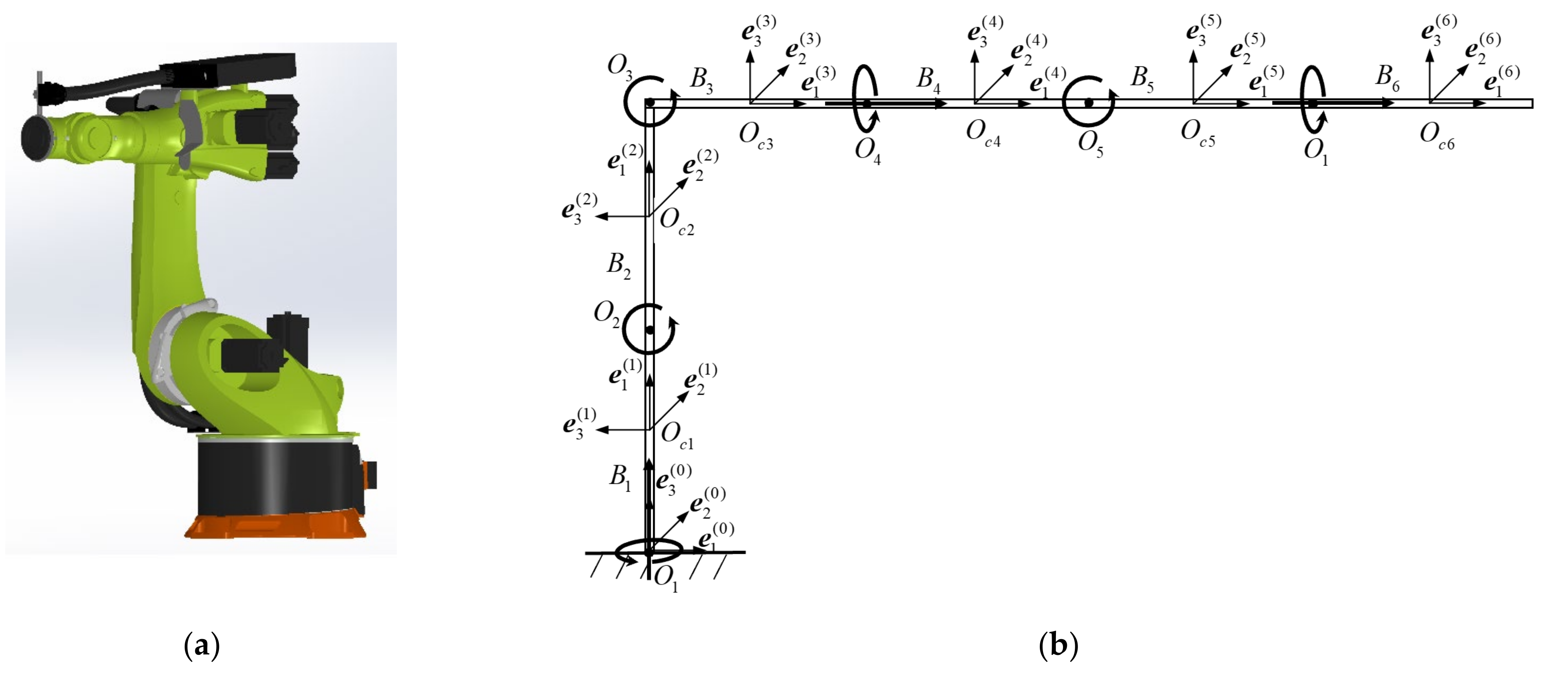
The 6-DOF robot has 6 rotational DOFs and consists of 6 rigid bodies and 6 hinges , where is the end effector, as shown in Figure 1. In order to facilitate analysis and calculation, each rigid body is simplified as a homogeneous cylinder with mass and central inertia tensor , each rigid body reference system is established at the position of the centroid , and the world reference system is established at the centroid of the bottom surface of the base . The directions of the base vectors are shown in Figure 1b.
The multibody system dynamic equation of the robot consists of the dynamic equations of each rigid body. Therefore, the dynamic equation of the rigid body should be established first. The dynamic equation of is derived according to the screw theory (the underlined represents the matrix form).
Here, , , , and are the generalized inertia matrix, twist, acceleration screw, and wrench of respectively, and is a 6-order square matrix.
and are the components of ’s velocity and acceleration in the direction, respectively; and are the components of ‘s angular velocity and angular acceleration in the direction, respectively (Superscript represents the expression relative to , and no superscript represents the expression relative to ); is the gravity force of ; , and are the force element and active moment that acts on , respectively, and there are force elements and moments associated with ; the body-hinge vector is the vector between the hinge point and the centroid, and the directions are from the inside to the outside, namely: ; the 3-order antisymmetric matrices and and the incidence element are defined as
In graph theory, the relationship between and is called incidence, starts with means that is the starting point of , and ends with means that is the end point of .
3.2. Dynamic Equation Based on Quaternion
Since the integral of angular velocity has no physical meaning, it cannot represent the angle. In practical applications, Euler angles, Cardano angles, Rodrigues parameters, or quaternions are selected as generalized angular coordinates. The first three all have singularities and are suitable for small-angle range motion. The quaternion has no singularity, is suitable for motion in a large angle range, and does not need to calculate the sine and cosine of the angle, which reduces the calculation steps and improves the calculation efficiency. For multi-DOF robots, quaternion coordinates are a better choice.
The angle in the dynamic Equation (1) of is expressed by the quaternion coordinate , and the quaternion and the position coordinate form the generalized coordinate . The generalized velocity and the generalized acceleration are derived from the first derivative and the second derivative of .
Twist and acceleration screw have the following relationships with generalized velocity and generalized acceleration ,
Here, is the Jacobian matrix
Therefore, the dynamic Equation (1) is expressed as
Here, is the generalized coordinate representation of ,
are defined as
The unconstrained rigid body has 3 rotational DOFs, while the quaternion has four parameters, so the quaternions are not independent parameters and have the following constraints,
In order to be combined with Equation (12), that is, to add constraint, Equation (15) needs to be derived twice with respect to time , and rewritten into the generalized coordinate form, where the following constraint is obtained,
Here,
Combining Equation (12) with Equation (17), that is, adding the quaternion self-constraint, the dynamic equation expressed by the generalized coordinate of is obtained,
Equation (18) can be abbreviated as
Here,
The dynamic equations Equation (19) of the 6 rigid bodies are combined to obtain the dynamic equation of the robot.
Here,
is a square matrix of order 42, and and are column matrices of order 42. The dynamic model Equation (21) of the robot has a total of 42 equations. The screw theory expresses the dynamic model of the robot as a set of equations. The form is simple and compact, which is convenient for calculation and control.
4. Quaternion-Based Constraint Equations
In the process of motion, there are certain relations between the generalized coordinates that describing the poses of each rigid body, and the analytical expressions of these relations are called constraint equations. A robot that satisfies the constraint equations can be controlled to move according to the true trajectory. The constraint equations of the robot are established by hinge constraints and quaternion self-constraints.
The robot has 6 rotation hinges, each of which has 1 rotational DOF and provides 5 constraints, namely 3 movement constraints and 2 rotation constraints. Furthermore, the angular coordinates that expressed by quaternions have their self-constraints. Specifically reflected as
(1) The hinge point of and its inside rigid body are the same point ,
is the coordinate transformation matrix that relative to ,
Equation (23) can be projected to the direction to obtain three projection expressions, corresponding to 3 movement constraints.
(2) The base vector of the rotation axis of and its inside rigid body is the same base vector ,
Equation (25) can be projected to the direction to obtain three projection expressions. Since the projections of the base vector in the directions have the relationship , only two of the three projection expressions are independent. Only take the projection expressions in the directions, corresponding to 2 rotation constraints.
(3) Quaternions are not independent parameters and are constrained by quaternion self-constraint Equation (15).
The constraint equations of the robot are obtained according to the projection expressions.
Each rigid body is subject to 5 kinematic constraints and 1 quaternion self-constraint, and a robot consisting of 6 rigid bodies has a total of 36 constraints. The dynamic Equation (21) of the robot has 42 equations and after being subjected to 36 constraints, the DOF is 6, which is consistent with the actual situation.
5. Constrained Dynamic Model of Robot
Only if the robot meets the constraints can its motion be in accord with the objective laws. The constraint equations are added to the dynamic Equation (21) by the Lagrange multiplier method, and the constrained dynamic model is obtained. The Lagrange multipliers are proportional to the ideal constraining force or moment.
The constraint equation of the robot is written as
Here, .
In order to be combined with Equation (21), the constraint Equation (62) needs to be written in the generalized acceleration form, therefore the Equation (62) is derived twice with respect to time , and the following equation is obtained,
Here, is the Jacobian matrix of , and the generalized coordinates of each rigid body constitute the robot’s generalized coordinate .
is the Jacobian matrix of .
According to the Lagrange multiplier method, first, 36 Lagrange multipliers are introduced into Equation (21) and combined into 6 Lagrange multiplier matrices , corresponding to the rigid body , respectively. constitutes the Lagrange matrix of the robot, from which the Lagrange equation of first kind is obtained.
Second, add constraints to Equation (65), that is, combine Equation (65) with constraint Equation (63).
Here, .
Equation (66) is the constrained dynamic model of the robot, with a total of 78 equations, which can solve up to 78 unknowns. The expression form of this equation is compact and unified, and the modular expression is easy to control. The force control or drive control of the robot can be realized by planning the trajectory curve of or , respectively. The Lagrange multiplier is proportional to the ideal constraining force or moment. By solving the Lagrange multipliers, the ideal constraining force and moment can be estimated, which can provide data and a theoretical basis for the analysis of the structural strength, reliability, and fatigue life of the robot.
6. Numerical Simulation Example
The robot is numerically simulated by Adams software to verify the correctness and accuracy of the dynamic Equation (66). As a precision machine, industrial robots are not easy to disassemble, which makes it impossible to measure the dynamic parameters of the rigid bodies that make up the robot by physical experiments, that is, the mass is obtained by weighing, and the principal moment of inertia is measured by the pendular motions. At the same time, the ideal constraint force and moment cannot be measured. Therefore, the mass , the principal moment of inertia ( are the components of in the direction, respectively), and the Lagrange multiplier of each rigid body are taken as the 78 unknown parameters to be calculated, and the remaining parameters are sampled as known parameters, then the unknown parameters are solved by Equation (66).
First, the three-dimensional model of the robot is established by Adams software and simulation experiments are carried out.
Each rigid body that composes the robot is simplified to a homogeneous cylindrical rod, the parameters of length and radius are provided, the material type is set to steel, and the value of gravitational acceleration is set to 9.80665. From these, the inertial parameters of the robot are generated, as shown in Table 1.
The purpose of the experiment is to solve the dynamic parameters and Lagrange multipliers of the robot. This means that the dynamic parameters and Lagrange multipliers of each rigid body are regarded as unknown parameters to be solved, and the other 6 parameters of each rigid body are regarded as known parameters, that is, the measured parameters, which are: (1) quaternion coordinates relative to ; (2) the force element exerted on by relative to ; (3) the active moment exerted on by relative to ; (4) the centroid acceleration relative to ; (5) the angular velocity relative to ; (6) the angular acceleration relative to .
In order to simplify the experiment and reduce the computational difficulty, the ideal experiment is to solve the dynamic parameters and Lagrange multipliers of the robot with only one movement, which means that the 6 rigid bodies that make up the robot can generate the 6 known parameters in this movement. Since the rigid bodies are connected to each other by hinges, the movement of the inner rigid body will drive the outer rigid body to move together. If the inner rigid body generates the 6 known parameters during the motion, the outer rigid body will generate the 6 known parameters at the same time. is connected to the ground and can only generate the angular acceleration in the direction, but cannot generate the angular acceleration in the direction, so needs to move at the same time to generate the angular acceleration in the direction. can generate the 6 known parameters in this movement, and also generates the 6 known parameters at the same time, so does not need to move relative to the inner rigid body.
Simulation settings: The initial state is static, and the posture is shown in Figure 1. Both hinge and hinge rotate at the angular acceleration of (namely ). The direction of the axis of rotation of hinge is , and the direction of the axis of rotation of hinge is , and other hinges are locked so that they do not rotate. The simulation termination time is 2 s, and the change of the robot’s posture during the movement is shown in Figure 2. The trajectories of the 6 measured parameters of each rigid body over time are shown in Appendix A.
Second, the data of the motion process is sampled, and then the unknown parameters are solved.
The 1.2 s time (or any other time) is selected to sample the data of the quaternion, force element , active moment , angular velocity, angular acceleration, and centroid acceleration of each rigid body. The sampled data is introduced into Equation (66) to calculate the results of unknown parameters. The calculation results are shown in Table 2 and Table 3.
(), (), () are the calculated masses of in the , , directions, respectively. Since is fixed to the ground, no acceleration occurs in the direction, so the mass cannot be obtained in these directions.
Finally, the calculated results are analyzed.
Comparing the true values of inertial parameters in Table 1 with the calculated values of inertial parameters in Table 2, the maximum absolute error of the two is −0.0723 . The error comes from the rounding of the significant figures of the data, and the increase of the number of calculations will lead to the accumulation of errors. The error cannot be eliminated, so the very small error verifies the correctness and accuracy of the dynamic model.
The Lagrange multipliers in Table 3 have clear physical meanings, where are proportional to the ideal constraining force of in the direction respectively; that introduced by the constraint Equation (25) are proportional to the ideal constraining moments; while introduced by the quaternion self-constraint Equation (15) does not reflect the ideal constraining moment.
The posture of the robot at 1.2 s is shown in Figure 2e. Since is affected by gravity, and the inner rigid body bears more gravity than the outer rigid body, therefore is much larger than and decreases with the increase of serial number .
The rotation axes of are all in the direction and need to bear the torque generated by gravity; the rotation axes of are not in the direction and do not need to bear the torque generated by gravity, so the ideal constraining moment of is large and the ideal constraining moment of is small. Therefore, the value of is much larger than that of . The number of outer rigid bodies of decreases, and the torque they received also decreases, so decreases with the increase of serial number . In the same way, the number of outer rigid bodies of decreases, and the torque they received also decreases, so decreases with the increase of serial number .
The data show that each rotating hinge of the robot receives great ideal constraining force in the vertical direction, while it receives very little ideal constraining force in the horizontal direction. When the direction of the hinge’s rotation axis is the same as the direction of the moment of the outer rigid body to the hinge, the hinge is subjected to a large ideal constraining moment; when the two directions are perpendicular, the ideal constraining moment of the hinge is small. The calculated values of Lagrange multipliers conform to objective physical laws, which also verifies the correctness of the dynamic model.
7. Conclusions
The dynamics of 6-DOF robot are systematically studied in this paper, and a dynamic modeling method of multibody system based on screw theory is proposed.
- (1)
- The dynamic and kinematic parameters of each rigid body can be decoupled by this method, and the dynamic model is concisely and compactly expressed as a modular matrix equation, which is convenient for both the solution of the dynamic model and the control.
- (2)
- Quaternions are used as generalized angular coordinates in this method, which eliminates singularities and makes the dynamic model suitable for motion in a large angular range. Additionally, the computational efficiency is improved.
- (3)
- The dynamic model established by this method is correct and accurate, which is verified by the numerical example. This method can provide a theoretical basis for the research on the dynamics of 6-DOF robot and its control method.
The future work is to carry out the research on related control methods.
Author Contributions
Conceptualization, J.C. and S.B.; methodology, J.C.; software, J.C.; validation, J.C. and S.B.; formal analysis, J.C., C.Y. and L.Z.; investigation, J.C. and C.Y.; resources, S.B.; data curation, J.C.; writing—original draft preparation, J.C.; writing—review and editing, J.C. and S.B.; visualization, C.Y.; supervision, S.B., Y.C. and Y.Y.; project administration, J.C. and C.Y.; funding acquisition, S.B. All authors have read and agreed to the published version of the manuscript.
Funding
This work was supported by “The National Key R&D Program of China (No. 2017YFB1301700)”.
Acknowledgments
We thank Weilong Fan for technical support.
Conflicts of Interest
The authors declare no conflict of interest.
Appendix A
The trajectories of the 6 measured parameters of each rigid body over time.
Figure A1.
The quaternion coordinates of each rigid body relative to . (a) the quaternion coordinates of ; (b) the quaternion coordinates of ; (c) the quaternion coordinates of ; (d) the quaternion coordinates of ; (e) the quaternion coordinates of ; (f) the quaternion coordinates of .
Figure A1.
The quaternion coordinates of each rigid body relative to . (a) the quaternion coordinates of ; (b) the quaternion coordinates of ; (c) the quaternion coordinates of ; (d) the quaternion coordinates of ; (e) the quaternion coordinates of ; (f) the quaternion coordinates of .

Here, quaternion0, quaternion1, quaternion2, quaternion3 are the four components of the quaternions, respectively.
Figure A2.
The force element exerted on by relative to . (a) the force element exerted on by ; (b) the force element exerted on by ; (c) the force element exerted on by ; (d) the force element exerted on by ; (e) the force element exerted on by ; (f) the force element exerted on by .
Figure A2.
The force element exerted on by relative to . (a) the force element exerted on by ; (b) the force element exerted on by ; (c) the force element exerted on by ; (d) the force element exerted on by ; (e) the force element exerted on by ; (f) the force element exerted on by .

Here, FX, FY, FZ are the three components of the force element in the direction, respectively.
Figure A3.
The active moment exerted on by relative to . (a) the active moment exerted on by ; (b) the active moment exerted on by ; (c) the active moment exerted on by ; (d) the active moment exerted on by ; (e) the active moment exerted on by ; (f) the active moment exerted on by .
Figure A3.
The active moment exerted on by relative to . (a) the active moment exerted on by ; (b) the active moment exerted on by ; (c) the active moment exerted on by ; (d) the active moment exerted on by ; (e) the active moment exerted on by ; (f) the active moment exerted on by .

Here, TX, TY, TZ are the three components of the active moment in the direction, respectively.
Figure A4.
The centroid acceleration of relative to . (a) the centroid acceleration of ; (b) the centroid acceleration of ; (c) the centroid acceleration of ; (d) the centroid acceleration of ; (e) the centroid acceleration of ; (f) the centroid acceleration of .
Figure A4.
The centroid acceleration of relative to . (a) the centroid acceleration of ; (b) the centroid acceleration of ; (c) the centroid acceleration of ; (d) the centroid acceleration of ; (e) the centroid acceleration of ; (f) the centroid acceleration of .

Here, cm_ACCX, cm_ACCY, cm_ACCZ are the three components of the centroid acceleration in the direction, respectively.
Figure A5.
The angular velocity of relative to . (a) the angular velocity of ; (b) the angular velocity of ; (c) the angular velocity of ; (d) the angular velocity of ; (e) the angular velocity of ; (f) the angular velocity of .
Figure A5.
The angular velocity of relative to . (a) the angular velocity of ; (b) the angular velocity of ; (c) the angular velocity of ; (d) the angular velocity of ; (e) the angular velocity of ; (f) the angular velocity of .

Here, WX, WY, WZ are the three components of the angular velocity in the direction, respectively.
Figure A6.
The angular acceleration of relative to . (a) the angular acceleration of ; (b) the angular acceleration of ; (c) the angular acceleration of ; (d) the angular acceleration of ; (e) the angular acceleration of ; (f) the angular acceleration of .
Figure A6.
The angular acceleration of relative to . (a) the angular acceleration of ; (b) the angular acceleration of ; (c) the angular acceleration of ; (d) the angular acceleration of ; (e) the angular acceleration of ; (f) the angular acceleration of .

Here, WDX, WDY, WDZ are the three components of the angular acceleration in the direction, respectively.
References
- Khalil, W.; Guegan, S. Inverse and direct dynamic modeling of Gough-Stewart robots. IEEE Trans. Robot. 2004, 20, 754–761. [Google Scholar] [CrossRef] [Green Version]
- Djuric, A.M.; El Maraghy, W.H. Automatic separation method for generation of reconfigurable 6R robot dynamics equations. Int. J. Adv. Manuf. Technol. 2010, 46, 831–842. [Google Scholar] [CrossRef]
- Ibrahim, O.; Khalil, W. Inverse and direct dynamic models of hybrid robots. Mech. Mach. Theory 2010, 45, 627–640. [Google Scholar] [CrossRef]
- Koopaee, M.J.; Pretty, C.; Classens, K.; Chen, X. Dynamical modeling and control of modular snake robots with series elastic actuators for pedal wave locomotion on uneven terrain. J. Mech. Des. 2020, 142, 031120. [Google Scholar] [CrossRef]
- Kalyoncu, M. Mathematical modelling and dynamic response of a multi-straight-line path tracing flexible robot manipulator with rotating-prismatic joint. Appl. Math. Model. 2008, 32, 1087–1098. [Google Scholar] [CrossRef]
- Li, H.; Yang, Z.; Huang, T. Dynamics and elasto-dynamics optimization of a 2-DOF planar parallel pick-and-place robot with flexible links. Struct. Multidiscip. Optim. 2009, 38, 195–204. [Google Scholar] [CrossRef]
- Dai, J.S. Screw Algebra and Kinematic Approaches for Mechanisms and Robotics; Springer: London, UK, 2014. [Google Scholar]
- Dai, J.S. Geometrical Foundations and Screw Algebra for Mechanisms and Robotics; Higher Education Press: Beijing, China, 2014. [Google Scholar]
- Sun, Y.; Wang, S.; Mills, J.K.; Zhi, C. Kinematics and dynamics of deployable structures with scissor-like-elements based on screw theory. Chin. J. Mech. Eng. 2014, 27, 655–662. [Google Scholar] [CrossRef]
- Müller, A. Screw and lie group theory in multibody dynamics. Multibody Syst. Dyn. 2018, 42, 219–248. [Google Scholar] [CrossRef] [Green Version]
- Cibicik, A.; Egeland, O. Dynamic modelling and force analysis of a knuckle boom crane using screw theory. Mech. Mach. Theory 2019, 133, 179–194. [Google Scholar] [CrossRef]
- Liu, W.; Gong, Z.; Wang, Q. Investigation on Kane dynamic equations based on screw theory for open-chain manipulators. Appl. Math. Mech. 2005, 26, 627–635. [Google Scholar]
- Pardos-Gotor, J.M. Screw Theory in Robotics: An Illustrated and Practicable Introduction to Modern Mechanics; CRC Press: Boca Raton, FL, USA, 2021. [Google Scholar]
- Lynch, K.M.; Park, F.C. Modern Robotics; Cambridge University Press: Cambridge, UK, 2017. [Google Scholar]
- Ajwad, S.A.; Ullah, M.I.; Islam, R.U.; Iqbal, J. Modeling robotic arms–A review and derivation of screw theory based kinematics. In Proceedings of the International Conference on Engineering and Emerging Technologies, Lahore, Pakistan, 1–2 December 2014; p. 98. [Google Scholar]
- Gallardo, J.; Rico, J.M.; Frisoli, A.; Checcacci, D.; Bergamasco, M. Dynamics of parallel manipulators by means of screw theory. Mech. Mach. Theory 2003, 38, 1113–1131. [Google Scholar] [CrossRef]
- Zhao, T.; Geng, M.; Chen, Y.; Li, E.; Yang, J. Kinematics and dynamics Hessian matrices of manipulators based on screw theory. Chin. J. Mech. Eng. 2015, 28, 226–235. [Google Scholar] [CrossRef]
- Gallardo-Alvarado, J.; Aguilar-Nájera, C.R.; Casique-Rosas, L.; Rico-Martínez, J.M.; Islam, M.N. Kinematics and dynamics of 2 (3-RPS) manipulators by means of screw theory and the principle of virtual work. Mech. Mach. Theory 2008, 43, 1281–1294. [Google Scholar] [CrossRef]
- Gallardo-Alvarado, J.; Rodríguez-Castro, R.; Delossantos-Lara, P.J. Kinematics and dynamics of a 4-PRUR Schönflies parallel manipulator by means of screw theory and the principle of virtual work. Mech. Mach. Theory 2018, 122, 347–360. [Google Scholar] [CrossRef]
- Gallardo-Alvarado, J.; Aguilar-Nájera, C.R.; Casique-Rosas, L.; Pérez-González, L.; Rico-Martínez, J.M. Solving the kinematics and dynamics of a modular spatial hyper-redundant manipulator by means of screw theory. Multibody Syst. Dyn. 2008, 20, 307–325. [Google Scholar] [CrossRef]
- Ding, X.; Selig, J.M. Dynamic modelling of a compliant arm with 6-dimensional tip forces using screw theory. Robotica 2003, 21, 193–197. [Google Scholar] [CrossRef]
Figure 1.
6-DOF robot and its schematic of the reference systems (a) 6-DOF robot; (b) schematic of the robot’s reference systems.
Figure 1.
6-DOF robot and its schematic of the reference systems (a) 6-DOF robot; (b) schematic of the robot’s reference systems.

Figure 2.
The postures at each time of the robot’s simulation model. (a) 0 s; (b) 0.3 s; (c) 0.6 s; (d) 0.9 s; (e) 1.2 s; (f) 1.5 s; (g) 1.8 s; (h) 2 s.
Figure 2.
The postures at each time of the robot’s simulation model. (a) 0 s; (b) 0.3 s; (c) 0.6 s; (d) 0.9 s; (e) 1.2 s; (f) 1.5 s; (g) 1.8 s; (h) 2 s.


Table 1.
Physical parameters of robot.
| ) | 1.045 | 1.245 | 1.21 | 0.315 | 0.29 | 0.3 |
| ) | 0.5 | 0.3 | 0.2 | 0.2 | 0.2 | 0.3 |
| ) | 6402.6012 | 2746.0726 | 1186.1661 | 308.7953 | 284.2877 | 661.7042 |
| ) | 800.3251 | 123.5733 | 23.7233 | 6.1759 | 5.6858 | 29.7767 |
| ) | 982.8126 | 416.4934 | 156.5838 | 5.6413 | 4.8353 | 19.8511 |
| ) | 982.8126 | 416.4934 | 156.5838 | 5.6413 | 4.8353 | 19.8511 |
Table 2.
The solved inertial parameters.
| ) | — | 2746.0726 | 1186.1658 | 308.7950 | 284.2880 | 661.7042 |
| ) | — | 2746.0685 | 1186.1663 | 308.7954 | 284.2878 | 661.7042 |
| ) | 6402.5982 | 2746.0727 | 1186.1656 | 308.7955 | 284.2878 | 661.7042 |
| ) | 800.3261 | 123.5681 | 23.7140 | 6.1793 | 5.6847 | 29.7768 |
| ) | 982.8122 | 416.4211 | 156.5920 | 5.6417 | 4.8364 | 19.8510 |
| ) | 982.8122 | 416.5364 | 156.5840 | 5.6406 | 4.8353 | 19.8511 |
Table 3.
The solved Lagrange multipliers.
Publisher’s Note: MDPI stays neutral with regard to jurisdictional claims in published maps and institutional affiliations. |
© 2022 by the authors. Licensee MDPI, Basel, Switzerland. This article is an open access article distributed under the terms and conditions of the Creative Commons Attribution (CC BY) license (https://creativecommons.org/licenses/by/4.0/).
Share and Cite
MDPI and ACS Style
Cheng, J.; Bi, S.; Yuan, C.; Cai, Y.; Yao, Y.; Zhang, L. Dynamic Modeling Method of Multibody System of 6-DOF Robot Based on Screw Theory. Machines 2022, 10, 499. https://0-doi-org.brum.beds.ac.uk/10.3390/machines10070499
AMA Style
Cheng J, Bi S, Yuan C, Cai Y, Yao Y, Zhang L. Dynamic Modeling Method of Multibody System of 6-DOF Robot Based on Screw Theory. Machines. 2022; 10(7):499. https://0-doi-org.brum.beds.ac.uk/10.3390/machines10070499
Chicago/Turabian StyleCheng, Jun, Shusheng Bi, Chang Yuan, Yueri Cai, Yanbin Yao, and Ling Zhang. 2022. "Dynamic Modeling Method of Multibody System of 6-DOF Robot Based on Screw Theory" Machines 10, no. 7: 499. https://0-doi-org.brum.beds.ac.uk/10.3390/machines10070499
Note that from the first issue of 2016, this journal uses article numbers instead of page numbers. See further details here.