Article

Deep Subdomain Transfer Learning with Spatial Attention ConvLSTM Network for Fault Diagnosis of Wheelset Bearing in High-Speed Trains

1
College of Mechanical and Vehicle Engineering, Hunan University, Changsha 410082, China
2
State Key Laboratory of Mechanical Behavior in Traffic Engineering Structure and System Safety, Shi-Jiazhuang Tiedao University, Shijiazhuang 050043, China
*
Author to whom correspondence should be addressed.
Submission received: 6 December 2022 / Revised: 12 February 2023 / Accepted: 16 February 2023 / Published: 17 February 2023
(This article belongs to the Special Issue Advances in Bearing Modeling, Fault Diagnosis, RUL Prediction)

Abstract

:
High-speed trains operate under varying conditions, leading to different distributions of vibration data collected from the wheel bearings. To detect bearing faults in situations where the source and target domains exhibit differing data distributions, the technique of transfer learning can be applied to move the distribution of features gleaned from unlabeled data in the source domain. However, traditional deep transfer learning techniques do not take into account the relationships between subdomains within the same class of different domains, resulting in suboptimal transfer learning performance and limiting the use of intelligent fault diagnosis for wheel bearings under various conditions. In order to tackle this problem, we have developed the Deep Subdomain Transfer Learning Network (DSTLN). This innovative approach transfers the distribution of features by harmonizing the subdomain distributions of layer activations specific to each domain through the implementation of the Local Maximum Mean Discrepancy (LMMD) method. The DSTLN consists of three modules: a feature extractor, fault category recognition, and domain adaptation. The feature extractor is constructed using a newly proposed SA-ConvLSTM model and CNNs, which aim to automatically learn features. The fault category recognition module is a classifier that categorizes the samples based on the extracted features. The domain adaptation module includes an adversarial domain classifier and subdomain distribution discrepancy metrics, making the learned features domain-invariant across both the global domain and subdomains. Through 210 transfer fault diagnosis experiments with wheel bearing data under 15 different operating conditions, the proposed method demonstrates its effectiveness.

1. Introduction

Fault diagnosis technology has gained increasing importance in recent years to enhance mechanical systems’ reliability and safety [1,2]. Monitoring the condition of operating mechanical equipment can help avoid severe financial losses and potential injuries [3]. Ensuring intense monitoring of key components of machinery operation and quickly and accurately identifying issues are critical to preventing catastrophic accidents. Rolling bearings play a significant role in a wide range of industries as vital components of rotating machinery [4,5]. Rolling bearing faults account for 51% of all rotating mechanical faults [6]. They are one of the main factors affecting the reliable and safe operation of mechanical systems [7]. The wheelset bearing of high-speed trains (HSTs), as a key part of high-speed train running parts, fails easily as a result of the long time spent in a complex wheel–rail excitement working status. A schematic diagram of a high-speed train wheelset bearing structure is shown in Figure 1. The failures cause serious damage to the safe operation of high-speed trains. Therefore, the development of relevant fault diagnosis techniques for high-speed train wheelset bearings is crucial and fundamental in ensuring the safe operation of rail transit [8,9].
The vibration generated during the operation of wheelset bearings is complex due to the intricate nature of the wheelset bearing system [10]. This vibration is primarily caused by both internal and external factors. Internally, the structural design of the bearing, manufacturing defects such as surface corrugations and roller size inconsistencies, assembly mistakes like shaft misalignment and unbalance, as well as operational problems, such as wear, pitting, poor lubrication, and the like, all contribute to the vibration. Externally, factors like track irregularity and special sections of track and wheel tread defects, among others, cause axle box-bearing vibrations and result in a complex interaction of wheel–rail excitations, with track irregularity being the primary cause. This has a significant impact on the ride comfort and safety of trains, particularly as train speed increases.
Traditional methods for diagnosing faults in wheelset bearings based on their vibration signals involve extracting the characteristic fault frequency. The approach to diagnosing bearing faults involves filtering the optimal fault band through digital signal processing techniques, such as filtering or decomposition [11,12,13], followed by an analysis of the envelope spectrum to identify different types of bearing faults. However, these methods often require specialized signal processing knowledge and manual feature extraction. Liu et al. [14] employed the multipoint kurtosis of the unbiased autocorrelation of the squared envelope signal to determine the most useful frequency range for high-speed rail wheelset bearings. Gu et al. proposed a Pareto optimum technique that maximizes the time domain and frequency domain spectral negentropy [15]. Additionally, they utilized a grey wolf optimizer to estimate the optimal posterior wavelet parameters by maximizing the negentropy of the squared envelope and its spectrum [16]. To further enhance the multi-objective fitness function, Yang et al. [17] created a general rule that prioritizes maximum sparsity in both the squared envelope and its spectrum. This rule was tested and validated on high-speed train wheelset bearings.
Despite their advantages, traditional methods of fault diagnosis have certain limitations, such as the requirement for prior knowledge during feature extraction and the processing of a large volume of data. To overcome these challenges, deep learning has emerged as a popular approach to fault diagnosis. This method enables automatic feature extraction, which has been demonstrated in various studies to effectively recognize the health state of machinery through processing large amounts of vibration data [18,19]. For instance, Lei et al. [20] presented a two-stage learning technique that incorporates an unsupervised two-layer neural network and softmax regression to extract features adaptively. Another study by Ling et al. proposed a simple and effective diagnostic method for bearing problems using a depth-separable volume [21]. This technique enhances the stability of the diagnostic model by extracting multiple properties from vibration signals from different directions. Peng et al. proposed a unique deeper 1-D convolutional neural network with residual learning that was validated using data from various operating situations of high-speed train wheelset bearings [22]. Additionally, Ban and his team established a multi-location and multi-kernel scale learning framework that utilizes skip connections in the neural network to address the high nonlinearity and strong coupling of bearing vibration signals [23]. Deep learning has proven to be an effective method in addressing the limitations of traditional fault diagnosis techniques by enabling automatic feature extraction and processing of large amounts of data.
In Figure 2, we observe the vibration waveforms in the time and frequency domains of a wheelset bearing with an inner ring failure, recorded at different speeds on a rolling test bench [24]. The time domain waveform (Figure 2a) reveals that as the speed increases, the vibration amplitude also rises, and the fault impact gradually becomes masked by other disturbances. Furthermore, the frequency domain waveform (Figure 2b) shows that with changes in speed, the distribution of energy across different frequency bands also changes, making it challenging to consistently identify bearing fault characteristics across varying working conditions.
The traditional deep learning approach has shown good results when the training and testing datasets have a similar distribution [25]. However, this approach faces challenges in the case of high-speed train wheelset bearings, which are frequently used under varying speeds and complex load conditions. The collected data from these conditions often have different distributions, making the traditional deep learning model unsuitable. Additionally, obtaining enough labeled samples from different running conditions to train a generalizable model is both difficult and expensive. To overcome these limitations, transfer learning has been introduced to address the challenges in diagnosing faults in high-speed train wheelset bearings. Guo [26] proposed a deep convolutional transfer learning network that uses MMD distance and an adversarial domain classifier on unlabeled data. He et al. [27] presented the KMST-based FT technique for transferring under changing operating conditions. Li et al. [28] proposed a deep transfer non-negativity constraint sparse autoencoder for automatically extracting latent features from unprocessed vibration signals. To address the challenge of diagnosing newly emerging faults, Li et al. [29] introduced adversarial transfer learning. He et al. [30] suggested a defect diagnosis method that combines transfer learning and generative adversarial networks to generate virtual samples. Zhang et al. [31] proposed a 1D-LDSAN model, which utilizes a 1-D lightweight convolutional neural network and the local maximum mean difference method to extract advanced features and match the probability distributions of source and target domain data. The model was validated using the CWRU dataset and showed promising results when trained with a small amount of unlabeled target domain data.
The traditional transfer learning strategies concentrate on harmonizing the source and target distributions as a whole, ignoring the inter-subdomain relationships within the same class across both domains. This leads to a confusion of distributions of target sample characteristics, causing poor transfer task diagnosis accuracy. As shown in Figure 3a, the features from the source and target domains are combined in the same global domain, but the features from various subdomains are mixed, making proper classification difficult. This was a common issue in previous global domain transfer learning, making it ineffective for the diagnosis of different working conditions in bearings.
For a more accurate diagnosis in the target domain, it is crucial to align the distribution of relevant subdomains within the same class in both the source and destination domains rather than just focusing on the global domain shift. As shown in Figure 3b, by aligning the relevant subdomains, the features from the same subdomain are separated and distinguished from those from different subdomains. This helps to improve the diagnosis accuracy in the target domain.
Due to the impact of wheel–rail excitation and the intricate internal structure, the vibration response of train wheelset bearings experiences significant fluctuations under varying operating conditions. The accuracy of fault diagnosis could be enhanced by incorporating subdomain transfer learning in the diagnosis of faults in high-speed train wheelset bearings.
Therefore, a novel Deep Subdomain Transfer Learning Network (DSTLN) has been proposed to enhance the transferability of features for transfer learning diagnostic tasks in high-speed train wheelset bearings. The DSTLN consists of a feature extractor, fault classification, and domain adaptation. The feature extractor module is designed to learn features autonomously. The fault classification module classifies samples into the correct categories based on the extracted features. The domain adaptation module, which includes an adversarial domain classifier and subdomain distribution discrepancy metrics, makes the learned features invariant in both the global and subdomain domains.
The contributions of this paper are summarized as follows:
(1)
The subdomain adaptation principle is applied to the intelligent fault detection of wheelset bearings, and the effectiveness of this principle is demonstrated using a deep learning model implementation.
(2)
A deep network model based on SA-ConvLSTM and CNNs is proposed, which uses distribution discrepancy metrics of the relevant subdomain and adversarial transfer method to achieve subdomain transfer learning for bearing fault diagnosis.
(3)
The performance of the proposed model is evaluated using several metrics on a dataset for wheelset bearings, and a visualization technique is used to understand the subdomain transfer learning feature learning process.
The structure of this paper is as follows: (1) In Section 2, the concept of subdomain transfer learning is thoroughly explained; (2) the design and workings of the Deep Subdomain Transfer Learning Network (DSTLN) are thoroughly discussed in Section 3; (3) the efficacy and superiority of the DSTLN on the wheelset bearing dataset are demonstrated in Section 4; (4) finally, the paper is summarized in Section 5.

2. Subdomain Transfer Learning Problem

In this section, the concept and principles of subdomain transfer learning are presented and discussed.

2.1. Unsupervised Subdomain Transfer Learning

It is necessary to first clarify some fundamental concepts about transfer learning and domains in order to explain the issue that needs to be solved. A source domain is D S = { ( x S i , y S i ) } i = 1 N s with sufficient N S labeled samples ( y i S R C is the label of x i s ,i.e., y i S = j means x i s belonging to the j th class, where C is the number of classes). The target domain is D T = { x T i } i = 1 N T of N T unlabeled samples. D S and D T are samples from different data distributions p and q , respectively, and p q . Unsupervised transfer learning involves designing a deep neural network y = f ( x ) that can extract useful knowledge from labeled samples in the source domain and apply it to correctly classify the unlabeled samples in the target domain. The success of transfer learning depends on a well-designed loss function, which can be formally represented as follows:
min f 1 n s i = 1 N s J ( f ( x i S ) , y i S ) ) + λ d ( p , q )
where J . , . denotes the cross-entropy loss function of the fault category recognition module and d . , . denotes domain adaption loss function. The trade-off parameter λ determines the weight given to each loss term during the training process, which balances the relative importance of the classification loss and the domain adaptation loss.
According to the category, the source domain D S and target domain D T are divided into C number of subdomains D S ( c ) and D T ( c ) , respectively. c { 1 , 2 , , C } is the class label. The distribution of sub-source domain D S ( c ) and target domain D T ( c ) are defined as p ( c ) and q ( c ) , respectively. The objective of subdomain transfer learning is to match the distributions of the specific subdomains that belong to the same category. The loss function for this type of transfer learning is based on the global domain transfer learning loss function and can be expressed as:
min f 1 n s i = 1 N s J ( f ( x i S ) , y i S ) ) + λ E c [ d ( p ( c ) , q ( c ) ) ]
where E c [ ] denotes the mathematical expectation of category.
Additionally, since the target domain samples lack proper labeling, pseudo labels are used to assign the samples to their respective classes. The Local Maximum Mean Discrepancy (LMMD) is introduced as a metric to differentiate between the source and target subdomains.

2.2. Local Maximum Mean Discrepancy (Distribution Discrepancy Metrics of Relevant Subdomain)

Maximum Mean Discrepancy (MMD) [32] is widely used to estimate the distance between the source and target distribution. As a nonparametric metric, it has been easily improved with respect to many variants, such as MK-MMD [33], J-MMD [34], etc., and applied to bearing transfer learning intelligent diagnosis. The MMD is formulated as below:
d H p , q E p ϕ x S E q ϕ x T H 2
where H represents the reproducing kernel Hilbert space (RKHS). ϕ denotes the feature map function which maps the input feature to RKHS.
Previous applications of Maximum Mean Discrepancy (MMD) in deep transfer learning primarily focused on aligning the global distribution, neglecting the relationship between the subdomains from the source and target domain within the same category. Given the importance of considering these relationships, the alignment of relevant subdomains should also be taken into account. To address this issue and align the distributions of relevant subdomains, a new metric, Local Maximum Mean Discrepancy (LMMD) [35], is proposed:
d H p , q E c E p ( c ) ϕ x S E q ( c ) ϕ x T H 2
where p ( c ) and q ( c ) denote the distributions of relevant subdomains D S ( c ) and D T ( c ) within the same category c, respectively. The goal of minimizing the discrepancy between the relevant subdomains is to bring their distributions closer and achieve alignment within the same category.
To apply the LMMD in a feedforward deep network model, we need to make some assumptions. In order to calculate the expectation E c [ ] , we assume that each sample belongs to each category on the basis of weight w c , and the weight w i c of the sample x i is calculated by formulation as:
w i c = y i c x j , y j D y j c
where y i c denotes the one-hot label vector of sample x i .
In this scenario, it’s easy to transfer the true label y i S of a sample from the source domain into a one-hot vector for calculation w i S c purposes, as the sample is labeled. However, in an unsupervised transfer learning task, the samples from the target domain are unlabeled, making it impossible to directly calculate their w i T c . To overcome this issue, we use the concept of pseudo labels. By using a category classifier module, we predict the label of the sample from the target domain and use it as the pseudo label. This allows us to categorize the sample. Additionally, the deep feature extraction network generates activations for samples from both the source and target domains, represented as z i S l i = 1 n S and z j T l j = 1 n T , respectively, in layer l. Then the reformulated formulation is as follows:
d l p , q = 1 C c = 1 C i = 1 n S j = 1 n S w i S c w j S c k z i S l , z j S l + i = 1 n T j = 1 n T w i T c w j T c k z i T l , z j T l 2 i = 1 n S j = 1 n T w i S c w j T c k z i S l , z j T l
where z l is the activation of the lth layer.

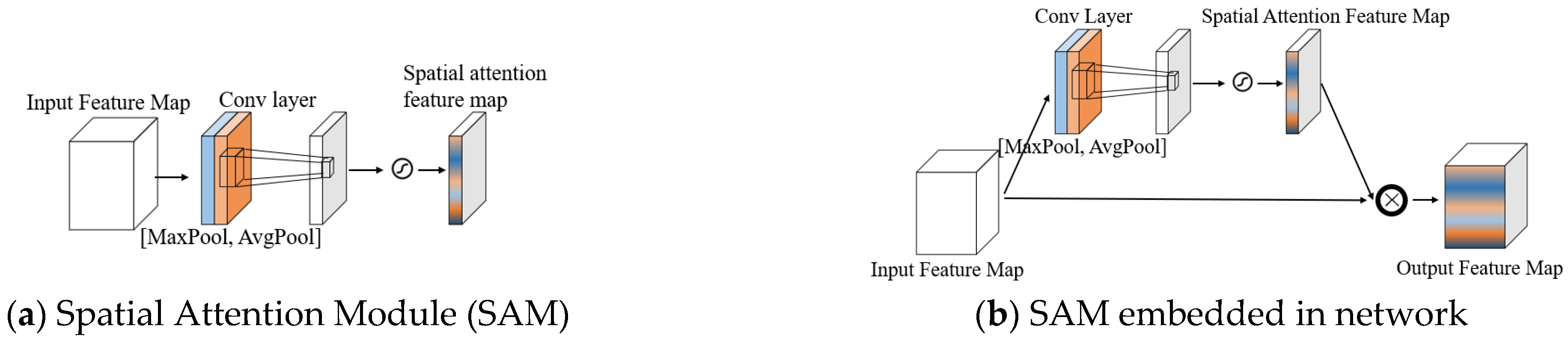
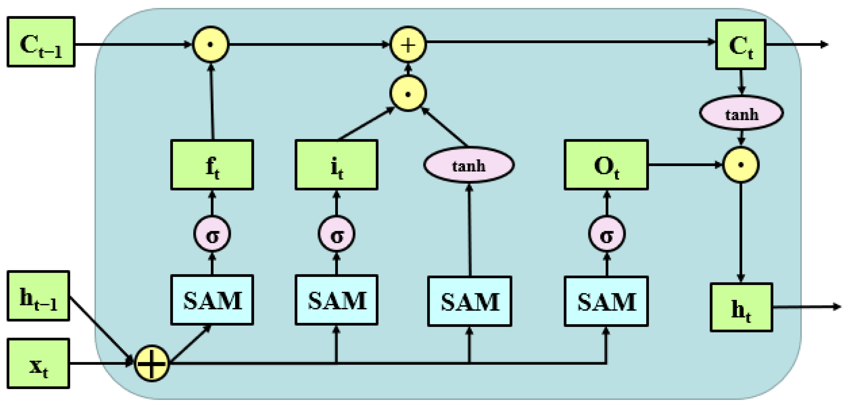
3. Spatial Attention ConvLSTM

In the preceding section, the theory and application of subdomain feature transfer for bearing fault diagnosis were described and established. To enhance the transfer capability of the model, it is essential to improve its feature extraction ability. Hence, this section introduces a new Spatial Attention ConvLSTM module aimed at augmenting the extraction of both temporal and spatial features. This module is designed to accommodate the cyclic stationarity characteristics and effects of bearing fault signals.

3.1. Spatial Attention Module

The Spatial Attention (SA) mechanism is designed to enhance the feature representation of key input parts of the neural network, resulting in improved global information extraction. Essentially, this mechanism transforms the original input into a new space through a spatial conversion module. The key information is then retained, and a weighted mask is generated for each position, resulting in a weighted output that strengthens relevant target-specific parts while reducing the impact of irrelevant parts. One prominent approach in this area is the Spatial Attention Module (SAM), introduced by Woo et al. [36]. It employs global mean and maximum pooling on channels, which then produce two feature representations through a 7 × 7 convolutional kernel, capturing different information aspects. Finally, the weight matrix is generated by Sigmoid operation, and the original input feature map is superimposed back. In this way, the purpose of enhancing the target region can be realized. Figure 4a shows the structure of the SAM module.
The expression formula of the Spatial Attention Module is represented as follows:
M s ( F ) = σ f 7 × 7 AvgPool F ; MaxPool F
where σ is the Sigmoid activation function, f 7 × 7 is the 7 × 7 convolutional kernel, AvgPool represents average pooling, MaxPool represents maximum pooling, F represents the input feature map, and Ms represents the output spatial attention feature map.
The SAM module can be seamlessly integrated into the neural network structure as a plug-in module, as illustrated in Figure 4b. It ultimately outputs an enriched feature map of the targeted region. The expression formula is presented below:
F M s ( F ) = M s F F
where is the Hadamard operator; F M s represents the output feature map after embedding the SAM.

3.2. Spatial Attention ConvLSTM

A spatial attention ConvLSTM (SA-ConvLSTM) model was proposed by introducing a spatial attention mechanism into the ConvLSTM [37] model, and its structure is shown as shown in Figure 5.
Different from image data, vibration data are generally one-dimensional data, so the convolution kernel in SAM is set to 1 × 7. The specific formula for SA-ConvLSTM is as follows:
i t = σ ( F M s ( W x i x t + W h i h t 1 + b i ) ) f t = σ ( F M s ( W x f x t + W h f h t 1 + b f ) ) o t = σ ( F M s ( W x o x t + W h o h t 1 + b o ) ) c t = f t c t 1 + i t tanh ( F M s ( W x c x t + W h c h t 1 + b c ) ) h t = o t tanh ( c t )
where represents the convolution operation; i , f , o , c , h , respectively, represent the input gate, the forgetting gate, the output gate, the memory unit, and the external state; σ ( )   is the Sigmoid function; is the Hadamard operator; and W represents the weight of neurons.

4. Proposed Method

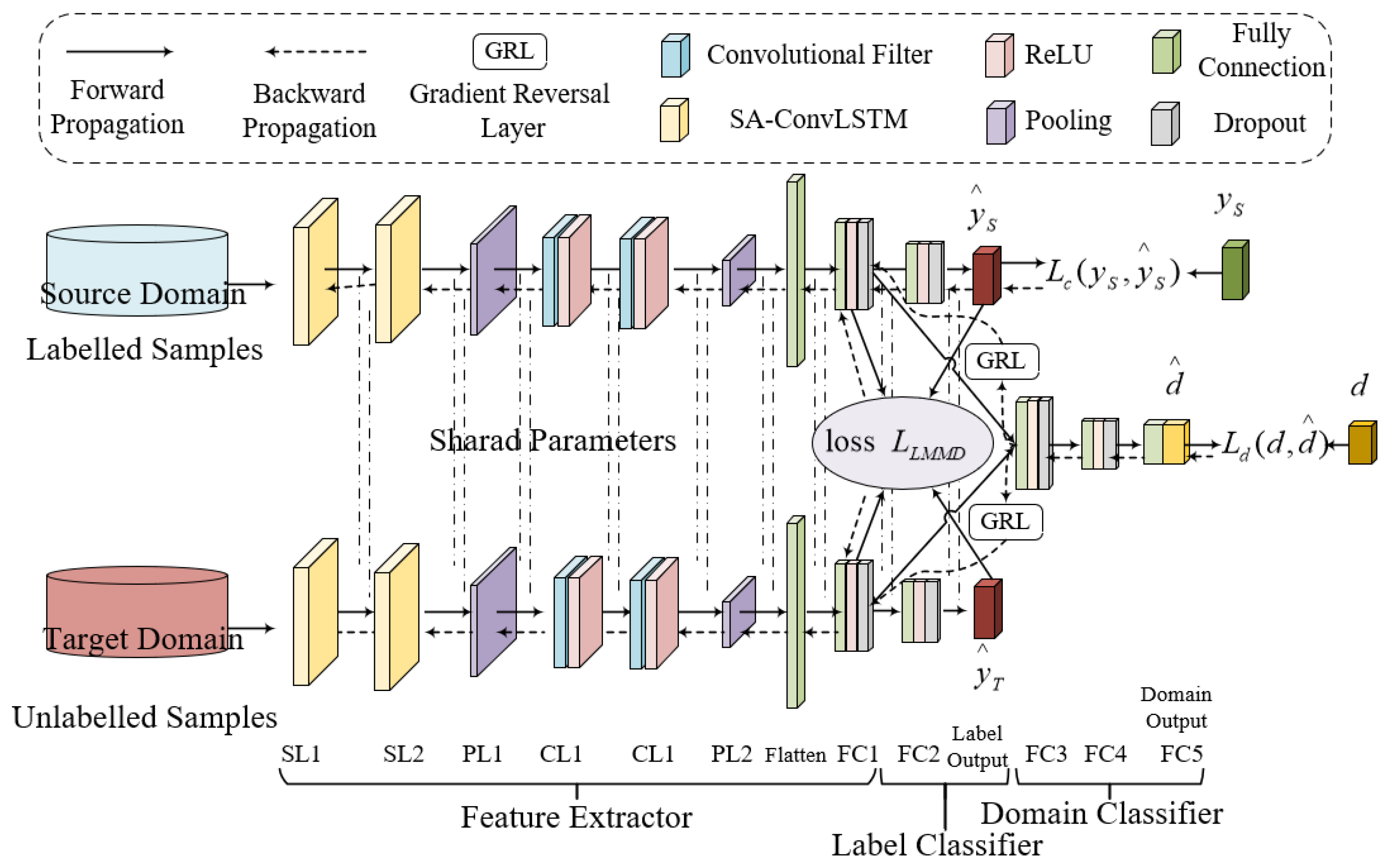
4.1. Deep Subdomain Transfer Learning Network (DSTLN)

The proposed DSTLN comprises three components: the feature extraction module, the fault category classification module, and the domain adaptation module. As depicted in Figure 6, the feature extraction module is composed of a CNN and SA-ConvLSTM capable of automatically learning features. The fault category recognition module is a classifier that assigns samples to their corresponding categories based on the extracted features. The domain adaptation module, which includes an adversarial domain classifier and subdomain distribution discrepancy metrics, helps make the learned features invariant across the global domain and subdomains. The specific parameters of each module are outlined in Table 1.
(1)
Feature extractor module
The feature extractor module is achieved by CNN and SA-ConvLSTM with seven layers, including two convolutional layers, two SA-ConvLSTM layers, two pooling layers, and one full-connected layer. This feature extractor module refers to a classical stackable convolutional neural network architecture [20], with a large convolution kernel in the first layer.
The feature extractor module takes vibration signals acquired by sensors mounted on equipment as inputs. Given that the vibration signals are one-dimensional data, the CNN layers are designed as 1-D CNN with ReLU function as the activation function. The output feature can be calculated using the following formula:
z l = ReLU d = 1 D W d l X d l + b l
where denotes the 1-D convolutional operator, W d denotes the weight of the convolutional kernel, X d denotes the input of the kernel, b l denotes the corresponding bias, and D is the number of kernels.
This module features two pooling layers, which serve a dual purpose. On one hand, they effectively reduce the number of neurons, while on the other hand, they help preserve the network’s stability in the face of small, local morphological changes. This allows the convolutional kernel to have a larger receptive field. The type of pooling used here is max pooling, which is formulated as follows:
p j = max { z j × k : ( j + 1 ) × k }
where k is the pooling length and pj is the output of the pooling operation.
After the CNN and pooling layer, a fully connected layer is added to flatten the output features. This is achieved through the following formulation:
z f l = ReLU W f l · X l + b l
where W f l is the weight matrix connecting two fully connected layers.
(2)
Label classification module
The label classification module comprises a fully connected layer and a softmax regression function. The inputs to layer FC2 are the output features from the feature extraction module. The output of layer FC2 is then fed into the softmax regression function, resulting in the final classification, as expressed by the following formulation:
y c = exp w c T x + b c c = 1 C exp w c T x + b c
where yc denotes the conditional probability of category c for the input x, and w c denotes the weight vector of category c.
(3)
Domain adaptation module
An adversarial domain classifier and a subdomain distribution discrepancy metrics term are both included in the domain adaption module.
The adversarial domain classifier is comprised of three layers. The first two layers are fully connected with ReLU activation and include dropout with a probability of 0.5. The third layer is a fully connected layer with a Sigmoid activation function. The output of these layers is then fed into a binary classifier setting using logistic regression, as expressed by the following formulation:
d = 1 1 + exp w d T x + b d
where w d denotes the weight matrix of the domain adaptation module and b d denotes the corresponding bias vector.
The subdomain distribution discrepancy metrics term is calculated referring to (6).

4.2. Optimization Objective

The proposed DSTLN is guided by three learning objective functions, as follows: (1) the health status classification error term on the source domain dataset; (2) the adversarial domain classification error term, applied to both the source and target domain datasets; and (3) the LMMD distribution discrepancy metric between the source and target domain datasets.
(1)
Object 1: Health status classification error term. The DSTLN aims to learn an invariant feature representation directly on the source domain dataset through the feature extractor module. As a result, the critical optimization objective of DSTLN is to minimize the health status classification error on data from the source domain. To achieve this, a typical softmax regression loss can be used as the expected objective function for a dataset with N categories of health status, as expressed below:
L c = 1 N i = 1 N J y i , y ^ i
where J(·) is the cross entropy function; y i is the predicted distribution of the ith sample across N fault categories and y ^ i is its real label.
(2)
Object 2: Adversarial domain classification error term. The adversarial domain classification error term serves a unique purpose in the DSTLN. The feature extractor is trained to deceive the domain classifier by maximizing this loss. In contrast, the adversarial domain classifier is educated to distinguish between the source domains by minimizing its loss. This ensures low classification errors in the source domain, all while minimizing the loss of the label classifier.
L d = 1 N S + N T i = 1 N S + N T J d i , d ^ i
(3)
Object 3: LMMD distribution discrepancy metrics term. The output Y of the label classifier module is used as the pseudo label of the target domain sample, and then the distribution difference of the subdomains is computed. By minimizing this function, aligning the distributions of relevant subdomains within the same category of the source and target domains is realized.
L L M M D = 1 C c = 1 C i = 1 n s w i s c ϕ ( x i s ) i = 1 n t w i t c ϕ ( x i t ) H 2
where ϕ denotes the kernel function; w i s c and w i t c denote the weight of x i s and x i t belonging to category C of the ith sample, respectively.
By combining these three optimization objectives, we obtain the final optimization objective as:
L = L c λ L d + μ L L M M D
where the trade-off parameters λ and μ determine the strength of the domain transfer effect.

4.3. Network Training Strategy

The following details outline the experiment training process. The trade-off parameters λ and μ are gradually increased from 0 to 1, calculated using the formula 2/(1 + exp(−10 × q)) − 1, where q represents the training progress, which is calculated as (current_epoch/max_epoch) and ranges from 0 to 1. The model is trained using the Adam optimizer, with a learning rate of 0.001 and a momentum parameter of 0.9. The batch size is 64, with each batch consisting of half samples from the source domain and half from the target domain. During each trial, half of the unlabeled data samples from the target domain and all of the labeled data samples from the source domain dataset are used as the training data. The remaining 20% and 30% of the target domain’s data samples are reserved for testing and validation, respectively. Algorithm 1 outlines the training process for the DSTLN.
Algorithm 1. DSTLN Training Strategy.
Input: source domain datasets with labels and target domain datasets without labels
Output: predict the fault class of the unlabeled target domain
Start
Step1: preprocessing of source domain and target domain datasets
Step2: creation of the neural network and initialization of the parameters randomly
Step3: input the preprocessed data to compute the Lc, Ld, and LLMMD, and compute the total Loss with the variable λ and μ according to current epoch
Step4: update network parameters by Adam optimizer, and Steps 3 and 4 should be repeated until the desired epoch is attained
Step5: save the trained model parameters to a file
Step6: utilizing the trained model, analyze the unlabeled target domain data
Step7: predict the fault category of the target domain for the input
End

5. Experiment Results and Comparisons

5.1. Experiment and Dataset

In this experiment, vibration signals were obtained from a high-speed train wheelset bearing as it underwent different load and speed conditions. The bench’s architecture for the high-speed train wheelset bearing is demonstrated in Figure 7, while Figure 8 illustrates the test bearing and the basic experimental setup. In Figure 8b, the sensor was positioned at the top of the test bearing’s end shield, and an accelerometer was used to capture the vibration signal. Table 2 presents the structural characteristics of the bearing.
To simulate the load changes experienced by a wheelset bearing during operation, various load forces are applied in both the vertical and axial directions to the test bearing. The load conditions include three scenarios: (1) An empty load; (2) a static load with 85 kN in the vertical direction and 50 kN in the axial direction; (3) a dynamic load with a vertical and axial frequency range of 0.2 to 20 Hz. The waveforms of these load forces are depicted in Figure 9.
To simulate the speed variations while that transpire during wheelset bearing operation, we experiment with a total of six operating condition speeds: static running speeds of 1200 r/min, 1500 r/min, 1800 r/min, and 2100 r/min, and a variable running speed ranging from 0 r/min to 2100 r/min and then to 0 r/min. As shown above, a total of 15 types of running conditions are tested on the test bearings. The details of each condition are shown in Table 3.
In each running condition, four test bearings are tested with different types of health conditions: (1) normal condition (NO); (2) outer race fault (OF); (3) inner race fault (IF); and (4) roller fault (RF). The damage location photographs are shown in Figure 10.
The sampling duration of each bearing is 60 s, with 51.2 kHz sampling frequency (Fs) in every running condition. The datasets are randomly split into training dataset, validation dataset, and test dataset, according to the ratio of 5:2:3. The sliding segmentation method is used for data augmentation [22,38,39]. In this experiment, the length of each sample is set as 2048, and the sliding step size is set as 256.
The DSTLN is implemented by the Pytorch machine learning framework and PythonTM 3.6. The model training and testing are performed on a workstation with an Intel® Xeon Gold 6148 CPU and a NVIDIA® GTX 2080Ti GPU with 11G memory. We compared the DSTLN with the following four other transfer learning methods. They are MK-MDD [40], JMMD [41], CORAL [42], and DANN [43].

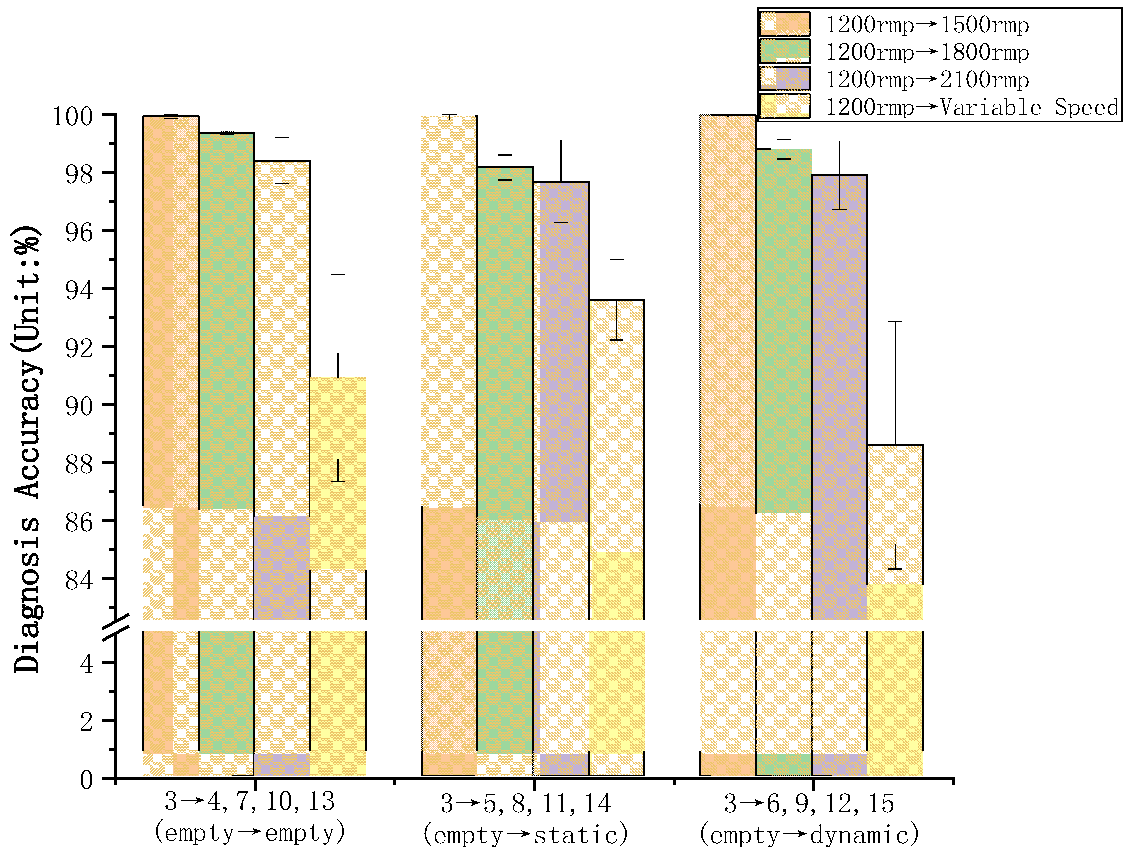
5.2. Transfer Fault Diagnosis of the DSTLN

The proposed DSTLN is assessed on a total of 210 transfer fault diagnosis experiments between each of the 15 condition datasets; i.e., 1 → 2, 2 → 1, 1 → 3, 3 → 1, and so on. The source domain in each transfer experiment is represented by the number before the arrow, while the target domain is indicated by the number following the arrow. For instance, in the transfer fault diagnostic experiment 1 → 15, the source domain corresponds to the first condition dataset, while the destination domain corresponds to the fifteenth condition dataset.
The neural network model’s parameters and structure are defined in Table 1 and Figure 6. The training step for each experiment is set to 1000, and each transfer experiment is run ten times at these specifications. The results of all 210 transfer experiments are presented in Table 4, with the row header indicating the target domain and the column header denoting the source domain’s working condition and data number. The accuracy of the transfer learning from the source domain to the target domain is presented in Table 4 as a percentage.
Table 4 demonstrates that the mutual transfer learning diagnosis results for the constant speed conditions exceed 99%, showcasing the effectiveness of the proposed DSTLN model in diagnosing various transfer learning scenarios.
As shown in Table 4, it can be observed that when the source and target domains have similar working conditions, the transfer diagnosis accuracy is higher. The transfer from working condition No. 3 to the other 12 working conditions is taken as an example. According to different load conditions, these transfer tests can be divided into three groups: 3 → 4,7,10,13 (empty → empty), 3 → 5,8,11,14 (empty → static), and 3 → 6,9,12,15 (empty → dynamic). The grouping results are plotted as shown in Figure 11 below. It can be observed that as the velocity difference increases, the accuracy of the transfer results decreases.
In addition, we found an interesting phenomenon when transfer learning between the constant speed and variable speed conditions. When transfer learning from the static speed condition to the variable speed condition, the accuracy of transfer learning diagnosis decreases significantly. On the other hand, when transfer learning from the dataset under variable speed condition to the dataset under constant speed condition, the accuracy of transfer learning diagnosis performance is good. We selected the forward and backward direction mutual transfer learning diagnosis results between variable speed condition No. 15 and the other 12 constant speed conditions for plotting, and the results are shown in Figure 12. We analyzed the reasons for the difference of transfer learning results in forward and backward directions. The reason is that the variable speed condition contains more comprehensive characteristic information. This instructs us to collect the data of complex conditions such as variable speed when setting the dataset and to use them as the training set in the source domain. In this way, higher accuracy can be obtained during transfer learning diagnosis.

5.3. Comparison Results
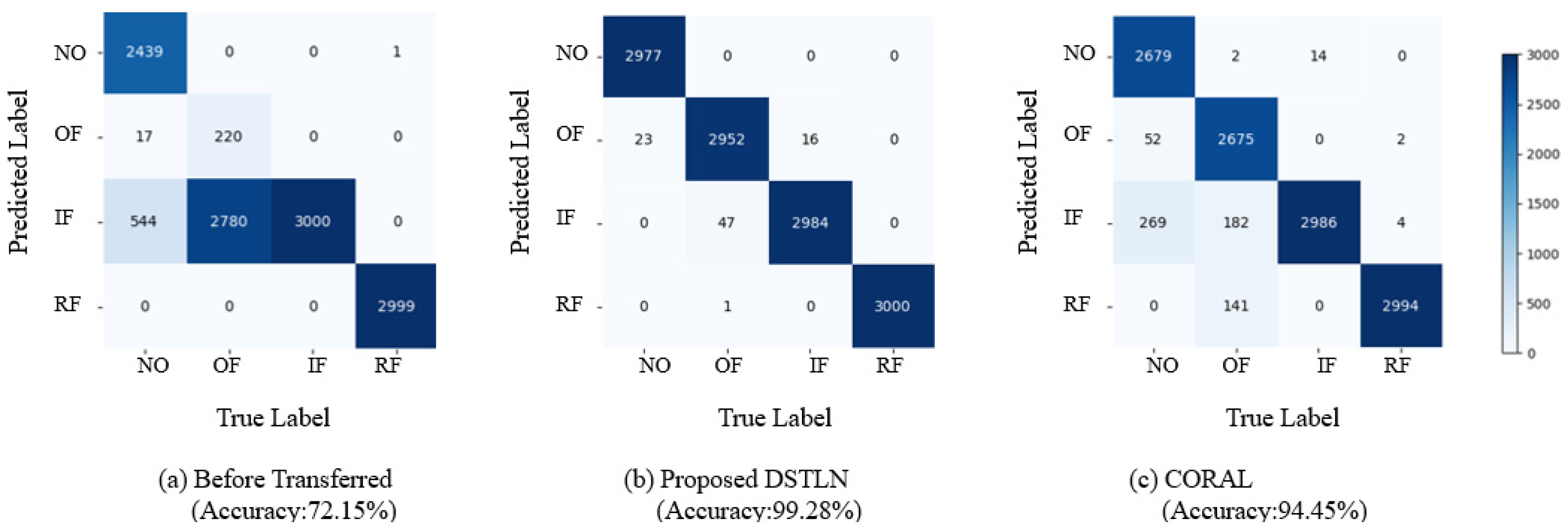
To further demonstrate the effectiveness of the proposed DSTLN, four additional transfer learning techniques are utilized for comparison in the same transfer fault diagnosis tests. These comparison methods utilize a feature extractor neural network with the same structure and parameters as the proposed DSTLN. The four comparison methods are multi-kernels MMD (MK-MMD) [40], Joint Maximum Mean Discrepancy (JMMD) [41], correlation alignment (CORAL) [42], and Domain-Adversarial Training of Neural Networks (DANN) [44].
We pick transfer experiment 1 → 5 as an example, which, with different speeds and loads, is common in 210 transfer conditions. The diagnosis accuracy results for the target domain and the confusion matrix are displayed in Figure 13. As shown in Figure 13a, prior to transfer, the diagnosis accuracy result without any labeled data from the target domain is only 72.15%. Figure 13b–f illustrate how transfer learning-based approaches outperform prior results for transfer diagnosis tasks. Moreover, the proposed DSTLN method outperforms all others, with a 99.28% accuracy.
Additionally, the t-distributed stochastic neighbor embedding (t-SNE) technique is applied to convert the high-dimensional features extracted by the final layer of the feature extractor module into a two-dimensional space to showcase the intricate relationships and patterns inherent in the data. The visualizations of these outcomes are detailed in Figure 14.
In particular, our comparison of the results led to the following three observations:
(1)
When analyzing the visualization result prior to transfer learning shown in Figure 14b, it becomes evident that the extracted features from the source domain are separated; however, the extracted features from the target domain differ from the source domain, and without transfer learning, the target domain’s distribution cannot be matched to the correct classifier, resulting in poor diagnosis accuracy. This indicates that without transfer learning, applying intelligent fault diagnosis of bearings with unlabeled data of varying working conditions may be challenging.
(2)
Compared to the result before the transfer, the transfer learning methods can align the identical class distributions in the source and target domains, as shown in Figure 14c–g. The transfer learning methods shift the target domain’s feature distribution to align with the source domain’s distribution. This suggests that the transfer learning methods effectively handle unlabeled data of varying working conditions.
(3)
As demonstrated in Figure 14d–g, other compared transfer learning techniques shift the feature distribution of the target domain to align with the source domain; however, they ignore the relationships between the subdomains with the same class in both domains. As a result, some data from the source and target domains are misclassified, and the distributions of the extracted features from different classes are mixed up, as depicted in Figure 15b. In contrast, the proposed DSTLN method aligns the distributions of relevant subdomains within the same class in both source and target domains, as shown in Figure 15a, resulting in improved diagnostic accuracy performance.

6. Conclusions

6.1. Conclusions of Results

In this paper, a novel approach of deep subdomain transfer learning is presented for the intelligent fault diagnosis of high-speed train wheelset bearings. The results of the experiments were compared to those obtained from four other transfer learning methods and were analyzed using t-SNE visualization.
The following conclusions were drawn from the experimental results:
(1)
Transfer learning-based intelligent fault diagnosis methods deliver higher diagnostic accuracy than deep learning methods without transfer learning processing, especially for bearing data with variable working conditions and no labels in the target domain.
(2)
The dataset under variable operating conditions comprises a more comprehensive set of characteristic information. A higher diagnostic accuracy can be achieved when it is set as the source domain dataset. This result can guide us to conduct further experiments under more variable speed and load force conditions. It can help us obtain a more comprehensive dataset for high-speed train wheelset bearings in the future.
(3)
The proposed DSTLN method captures fine-grained information. It aligns the distributions of relevant subdomains within the same source and target domain category, resulting in better diagnostic accuracy performance than other global domain transfer learning methods.
These conclusions demonstrate that the proposed DSTLN method can effectively classify unlabeled target domain data under different working conditions. As a result, DSTLN can potentially promote the successful application of intelligent fault diagnosis for high-speed train wheelset bearings with unlabeled data in variable working conditions.

6.2. Discussions of Future Work

Our research aims to develop a wheelset bearing diagnosis system for real-time monitoring of high-speed trains’ performance. However, there is still a long road ahead to reach this objective. The limitations and future work of our study are as follows:
(1)
Limitation of the wheelset bearing data. Although we conducted experiments on four healthy bearings under 15 different working conditions, it is still insufficient to cover all possible scenarios of real running high-speed trains. Our current testing rig cannot simulate rail–wheel excitement, which significantly impacts the vibration signals. In the future, we aim to conduct more experiments using our new roller test rig based on a real high-speed train bogie to acquire more accurate vibration data.
(2)
Metric measuring the transferability between different datasets for transfer learning. In our study, we used t-SNE visualization to understand the distribution of source and target datasets. However, we still need a quantitative measure of transferability between datasets. In the future, we plan to develop a quantitative measure to help us organize a complete dataset and avoid negative transfer learning.
(3)
Development of an embedded diagnostic system. Our proposed diagnostic method was implemented on a personal computer, which is both expensive and energy intensive. In the future, we aim to design and develop a more cost-effective and energy-efficient diagnostic model that can be deployed on an embedded system.

Author Contributions

Conceptualization, J.W., Y.L. and S.Y.; methodology, J.W. and Y.L.; software, J.W.; validation, Y.L. and G.W.; formal analysis, J.W.; investigation, J.W.; resources, Y.L.; data curation, Y.L.; writing—original draft preparation, J.W.; writing—review and editing, S.Y.; visualization, Y.L.; supervision, G.W.; project administration, S.Y.; funding acquisition, S.Y. All authors have read and agreed to the published version of the manuscript.

Funding

This work is supported by the National Natural Science Foundation of China (Nos. 12032017, 11790282, 11802184, 11902205 and 12002221), Key Scientific Research Projects of China Railway Group (N2021J032), S&T Program of Hebei (20310803D), and Natural Science Foundation of Hebei Province (No. A2020210028).

Institutional Review Board Statement

Not applicable.

Informed Consent Statement

Not applicable.

Data Availability Statement

Not applicable.

Conflicts of Interest

The authors declare no conflict of interest.

References

  1. Chen, H.; Shi, L.; Zhou, S.; Yue, Y.; An, N. A Multi-Source Consistency Domain Adaptation Neural Network MCDANN for Fault Diagnosis. Appl. Sci. 2022, 12, 10113. [Google Scholar] [CrossRef]
  2. Rezazadeh, N.; De Luca, A.; Lamanna, G.; Caputo, F. Diagnosing and Balancing Approaches of Bowed Rotating Systems: A Review. Appl. Sci. 2022, 12, 9157. [Google Scholar] [CrossRef]
  3. Wu, G.; Yan, T.; Yang, G.; Chai, H.; Cao, C. A Review on Rolling Bearing Fault Signal Detection Methods Based on Different Sensors. Sensors 2022, 22, 8330. [Google Scholar] [CrossRef] [PubMed]
  4. Jiang, X.; Wang, J.; Shi, J.; Shen, C.; Huang, W.; Zhu, Z. A coarse-to-fine decomposing strategy of VMD for extraction of weak repetitive transients in fault diagnosis of rotating machines. Mech. Syst. Signal Process. 2019, 116, 668–692. [Google Scholar] [CrossRef]
  5. Peng, H.; Zhang, H.; Fan, Y.; Shangguan, L.; Yang, Y. A Review of Research on Wind Turbine Bearings’ Failure Analysis and Fault Diagnosis. Lubricants 2023, 11, 14. [Google Scholar] [CrossRef]
  6. Manjurul Islam, M.M.; Kim, J.-M. Reliable multiple combined fault diagnosis of bearings using heterogeneous feature models and multiclass support vector Machines. Reliab. Eng. Syst. Saf. 2019, 184, 55–66. [Google Scholar] [CrossRef]
  7. Peng, B.; Bi, Y.; Xue, B.; Zhang, M.; Wan, S. A Survey on Fault Diagnosis of Rolling Bearings. Algorithms 2022, 15, 347. [Google Scholar] [CrossRef]
  8. Kuncan, M.; Kaplan, K.; Minaz, M.R.; Kaya, Y.; Ertunç, H.M. A novel feature extraction method for bearing fault classification with one dimensional ternary patterns. ISA Trans. 2020, 100, 346–357. [Google Scholar] [CrossRef]
  9. Jiao, Y.; Zhang, Y.; Ma, S.; Sang, D.; Zhang, Y.; Zhao, J.; Liu, Y.; Yang, S. Role of secondary phase particles in fatigue behavior of high-speed railway gearbox material. Int. J. Fatigue 2020, 131, 105336. [Google Scholar] [CrossRef]
  10. Liu, Z.; Yang, S.; Liu, Y.; Lin, J.; Gu, X. Adaptive correlated Kurtogram and its applications in wheelset-bearing system fault diagnosis. Mech. Syst. Signal Process. 2021, 154, 107511. [Google Scholar] [CrossRef]
  11. Liu, J.; Wang, W.; Golnaraghi, F. An Extended Wavelet Spectrum for Bearing Fault Diagnostics. IEEE Trans. Instrum. Meas. 2008, 57, 2801–2812. [Google Scholar] [CrossRef]
  12. Liu, D.; Cheng, W.; Wen, W. Rolling bearing fault diagnosis via STFT and improved instantaneous frequency estimation method. Procedia Manuf. 2020, 49, 166–172. [Google Scholar] [CrossRef]
  13. Mejia-Barron, A.; Valtierra-Rodriguez, M.; Granados-Lieberman, D.; Olivares-Galvan, J.C.; Escarela-Perez, R. The application of EMD-based methods for diagnosis of winding faults in a transformer using transient and steady state currents. Measurement 2018, 117, 371–379. [Google Scholar] [CrossRef]
  14. Liu, W.; Yang, S.; Li, Q.; Liu, Y.; Hao, R.; Gu, X. The Mkurtogram: A Novel Method to Select the Optimal Frequency Band in the AC Domain for Railway Wheelset Bearings Fault Diagnosis. Appl. Sci. 2021, 11, 9. [Google Scholar] [CrossRef]
  15. Gu, X.H.; Yang, S.P.; Liu, Y.Q.; Hao, R.J. A novel Pareto-based Bayesian approach on extension of the infogram for extracting repetitive transients. Mech. Syst. Signal Process. 2018, 106, 119–139. [Google Scholar] [CrossRef]
  16. Gu, X.; Yang, S.; Liu, Y.; Hao, R.; Liu, Z. Multi-objective Informative Frequency Band Selection Based on Negentropy-induced Grey Wolf Optimizer for Fault Diagnosis of Rolling Element Bearings. Sensors 2020, 20, 1845. [Google Scholar] [CrossRef] [PubMed] [Green Version]
  17. Yang, S.; Gu, X.; Liu, Y.; Hao, R.; Li, S. A general multi-objective optimized wavelet filter and its applications in fault diagnosis of wheelset bearings. Mech. Syst. Signal Process. 2020, 145, 106914. [Google Scholar] [CrossRef]
  18. Zhang, S.; Zhang, S.; Wang, B.; Habetler, T.G. Deep Learning Algorithms for Bearing Fault Diagnostics—A Comprehensive Review. IEEE Access 2020, 8, 29857–29881. [Google Scholar] [CrossRef]
  19. You, K.; Qiu, G.; Gu, Y. Rolling Bearing Fault Diagnosis Using Hybrid Neural Network with Principal Component Analysis. Sensors 2022, 22, 8906. [Google Scholar] [CrossRef]
  20. Lei, Y.; Jia, F.; Lin, J.; Xing, S.; Ding, S.X. An Intelligent Fault Diagnosis Method Using Unsupervised Feature Learning Towards Mechanical Big Data. IEEE Trans. Ind. Electron. 2016, 63, 3137–3147. [Google Scholar] [CrossRef]
  21. Ling, L.; Wu, Q.; Huang, K.; Wang, Y.; Wang, C. A Lightweight Bearing Fault Diagnosis Method Based on Multi-Channel Depthwise Separable Convolutional Neural Network. Electronics 2022, 11, 4110. [Google Scholar] [CrossRef]
  22. Peng, D.; Liu, Z.; Wang, H.; Qin, Y.; Jia, L. A Novel Deeper One-Dimensional CNN With Residual Learning for Fault Diagnosis of Wheelset Bearings in High-Speed Trains. IEEE Access 2019, 7, 10278–10293. [Google Scholar] [CrossRef]
  23. Ban, H.; Wang, D.; Wang, S.; Liu, Z. Multilocation and Multiscale Learning Framework with Skip Connection for Fault Diagnosis of Bearing under Complex Working Conditions. Sensors 2021, 21, 3226. [Google Scholar] [CrossRef]
  24. Liu, P.; Yang, S.; Liu, Y.; Gu, X.; Liu, Z.; Liu, H. An excitation test and dynamic simulation of wheel polygon wear based on a rolling test rig of single wheelset. Zhendong Chongji/J. Vib. Shock 2022, 41, 102–109. [Google Scholar] [CrossRef]
  25. He, Z.Y.; Shao, H.D.; Zhong, X.; Zhao, X.Z. Ensemble transfer CNNs driven by multi-channel signals for fault diagnosis of rotating machinery cross working conditions. Knowl. -Based Syst. 2020, 207, 106396. [Google Scholar] [CrossRef]
  26. Guo, L.; Lei, Y.; Xing, S.; Yan, T.; Li, N. Deep Convolutional Transfer Learning Network: A New Method for Intelligent Fault Diagnosis of Machines With Unlabeled Data. IEEE Trans. Ind. Electron. 2019, 66, 7316–7325. [Google Scholar] [CrossRef]
  27. He, Y.; Hu, M.; Feng, K.; Jiang, Z. An Intelligent Fault Diagnosis Scheme Using Transferred Samples for Intershaft Bearings Under Variable Working Conditions. IEEE Access 2020, 8, 203058–203069. [Google Scholar] [CrossRef]
  28. Li, X.; Jiang, H.; Zhao, K.; Wang, R. A Deep Transfer Nonnegativity-Constraint Sparse Autoencoder for Rolling Bearing Fault Diagnosis With Few Labeled Data. IEEE Access 2019, 7, 91216–91224. [Google Scholar] [CrossRef]
  29. Li, J.; Huang, R.; He, G.; Wang, S.; Li, G.; Li, W. A Deep Adversarial Transfer Learning Network for Machinery Emerging Fault Detection. IEEE Sens. J. 2020, 20, 8413–8422. [Google Scholar] [CrossRef]
  30. He, W.; Chen, J.; Zhou, Y.; Liu, X.; Chen, B.; Guo, B. An Intelligent Machinery Fault Diagnosis Method Based on GAN and Transfer Learning under Variable Working Conditions. Sensors 2022, 22, 9175. [Google Scholar] [CrossRef]
  31. Zhang, R.; Gu, Y. A Transfer Learning Framework with a One-Dimensional Deep Subdomain Adaptation Network for Bearing Fault Diagnosis under Different Working Conditions. Sensors 2022, 22, 1624. [Google Scholar] [CrossRef]
  32. Gretton, A.; Borgwardt, K.M.; Rasch, M.J.; Scholkopf, B.; Smola, A. A Kernel Two-Sample Test. J. Mach. Learn. Res. 2012, 13, 723–773. [Google Scholar]
  33. Gretton, A.; Sriperumbudur, B.; Sejdinovic, D.; Strathmann, H.; Balakrishnan, S.; Pontil, M.; Fukumizu, K. Optimal kernel choice for large-scale two-sample tests. In Proceedings of the 25th International Conference on Neural Information Processing Systems, Lake Tahoe, NV, USA, 3–6 December 2012; Volume 1, pp. 1205–1213. [Google Scholar]
  34. Long, M.; Zhu, H.; Wang, J.; Jordan, M.I. Deep transfer learning with joint adaptation networks. In Proceedings of the Proceedings of the 34th International Conference on Machine Learning, Sydney, NSW, Australia, 6–11 August 2017; Volume 70, pp. 2208–2217. [Google Scholar]
  35. Zhu, Y.; Zhuang, F.; Wang, J.; Ke, G.; Chen, J.; Bian, J.; Xiong, H.; He, Q. Deep Subdomain Adaptation Network for Image Classification. IEEE Trans. Neural Netw. Learn. Syst. 2021, 32, 1713–1722. [Google Scholar] [CrossRef] [PubMed]
  36. Woo, S.; Park, J.; Lee, J.-Y.; Kweon, I.S. CBAM: Convolutional Block Attention Module. arXiv 2018, arXiv:1807.06521. [Google Scholar]
  37. Shi, X.; Chen, Z.; Wang, H.; Yeung, D.Y.; Wong, W.K.; Woo, W.C. Convolutional LSTM Network: A Machine Learning Approach for Precipitation Nowcasting. Adv. Neural Inf. Process. Syst. 2015, 28, 802–810. [Google Scholar]
  38. Zhang, W.; Peng, G.; Li, C.; Chen, Y.; Zhang, Z. A New Deep Learning Model for Fault Diagnosis with Good Anti-Noise and Domain Adaptation Ability on Raw Vibration Signals. Sensors 2017, 17, 425. [Google Scholar] [CrossRef] [PubMed] [Green Version]
  39. Meng, Z.; Guo, X.; Pan, Z.; Sun, D.; Liu, S. Data Segmentation and Augmentation Methods Based on Raw Data Using Deep Neural Networks Approach for Rotating Machinery Fault Diagnosis. IEEE Access 2019, 7, 79510–79522. [Google Scholar] [CrossRef]
  40. Yang, B.; Li, Q.; Chen, L.; Shen, C. Bearing Fault Diagnosis Based on Multilayer Domain Adaptation. Shock Vib. 2020, 2020, 8873960. [Google Scholar] [CrossRef]
  41. Jj, A.; Ming, Z.A.; Jing, L.B.; Kl, A. Residual joint adaptation adversarial network for intelligent transfer fault diagnosis. Mech. Syst. Signal Process. 2020, 145, 106962. [Google Scholar]
  42. An, J.; Ai, P. Deep Domain Adaptation Model for Bearing Fault Diagnosis with Riemann Metric Correlation Alignment. Math. Probl. Eng. 2020, 2020, 1–12. [Google Scholar] [CrossRef] [Green Version]
  43. Zhao, Z.; Zhang, Q.; Yu, X.; Sun, C.; Wang, S.; Yan, R.; Chen, X. Unsupervised Deep Transfer Learning for Intelligent Fault Diagnosis: An Open Source and Comparative Study. arXiv 2019, arXiv:1912.12528. [Google Scholar]
  44. Wan, L.; Li, Y.; Chen, K.; Gong, K.; Li, C. A novel deep convolution multi-adversarial domain adaptation model for rolling bearing fault diagnosis. Measurement 2022, 191, 110752. [Google Scholar] [CrossRef]
Figure 1. Schematic diagram of a high-speed train wheelset bearing structure.
Machines 11 00304 g001
Figure 2. Time domain and frequency domain waveforms of wheelset bearings at different speeds.
Machines 11 00304 g002
Figure 3. (a) Global domain transfer learning can’t achieve the alignment of the distribution for the same class. (b) relevant subdomain transfer learning can align the distribution of the same class and make the subdomain be separated for each category. (The dots and stars represent different categories, with the stars representing class 1 and the dots representing class 2; different colors represent different domains, with blue representing source domain characteristics and red representing target domain characteristics).
Machines 11 00304 g003
Figure 4. Spatial Attention Module and SAM module embedded in the neural network structure.
Machines 11 00304 g004
Figure 5. Spatial attention ConvLSTM (SA-ConvLSTM) model structure.
Machines 11 00304 g005
Figure 6. Architecture of the proposed DSTLN, including three modules: feature extractor, label classifier, and domain classifier; and LMMD loss function is used to achieve subdomain transfer learning.
Machines 11 00304 g006
Figure 7. The test bench’s architecture for the high-speed train wheelset bearing.
Machines 11 00304 g007
Figure 8. (a) high-speed train wheelset bearing test bench; (b) local expanded test point; (c) test bearing.
Machines 11 00304 g008
Figure 9. Three loading forces. (a) axial direction; (b) vertical direction.
Machines 11 00304 g009
Figure 10. The damage location. (a) outer ring; (b) inner ring; (c) roller element.
Machines 11 00304 g010
Figure 11. The results between condition No. 3 and the other 12 conditions divided into three groups based on the same load conditions.
Machines 11 00304 g011
Figure 12. The results between variable speed condition No. 15 and the other 12 constant speed conditions.
Machines 11 00304 g012
Figure 13. The diagnosis accuracy of target domain and confusion matrix results. (Results of before transferred, proposed DSTLN and other four contrast methods have been demonstrated, and the proposed DSTLN outperforms the others.)
Machines 11 00304 g013aMachines 11 00304 g013b
Figure 14. The t-SNE visualization of the learned features in a high-speed train wheelset bearing dataset.
Machines 11 00304 g014
Figure 15. Comparison of subdomain and global domain transfer learning.( Proposed DSTLN method aligns the distributions of relevant subdomains within the same class in both source and target domains.)
Machines 11 00304 g015
Table 1. Architecture and parameter settings for the DSTLN.
ModulesLayersTied ParametersActivation Function
Feature
Extractor
SL1SA-ConvLSTM1d 20@32 -
SL2SA-ConvLSTM1d 20@3-
PL1Max Polling: kernel = 2, stride = 2-
CL1Conv1d 64@3ReLU
CL2Conv1d 128@3ReLU
PL2Max Pooling: kernel = 4, stride = 4-
FC1Output 256 featuresReLU
Label
Classifier
FC2Output 256 features; Dropout 0.5Softmax
Domain
Classifier
FC3Output 1024 features; Dropout 0.5ReLU
FC4Output 512 features; Dropout 0.5ReLU
FC5Output 2 featuresSigmoid
Table 2. Parameters of the bearing.
NameRoller DiameterPitch DiameterContact AngleRoller Number
FAG F-8078110926.5 mm185 mm10 deg17
Table 3. Condition number of each running condition.
Condition NumberSpeed (km/h)
2002503003500 → 350 → 0
LoadEmpty load1471013
Static load
(Vertical 85 kN; axial 50 kN)
2581114
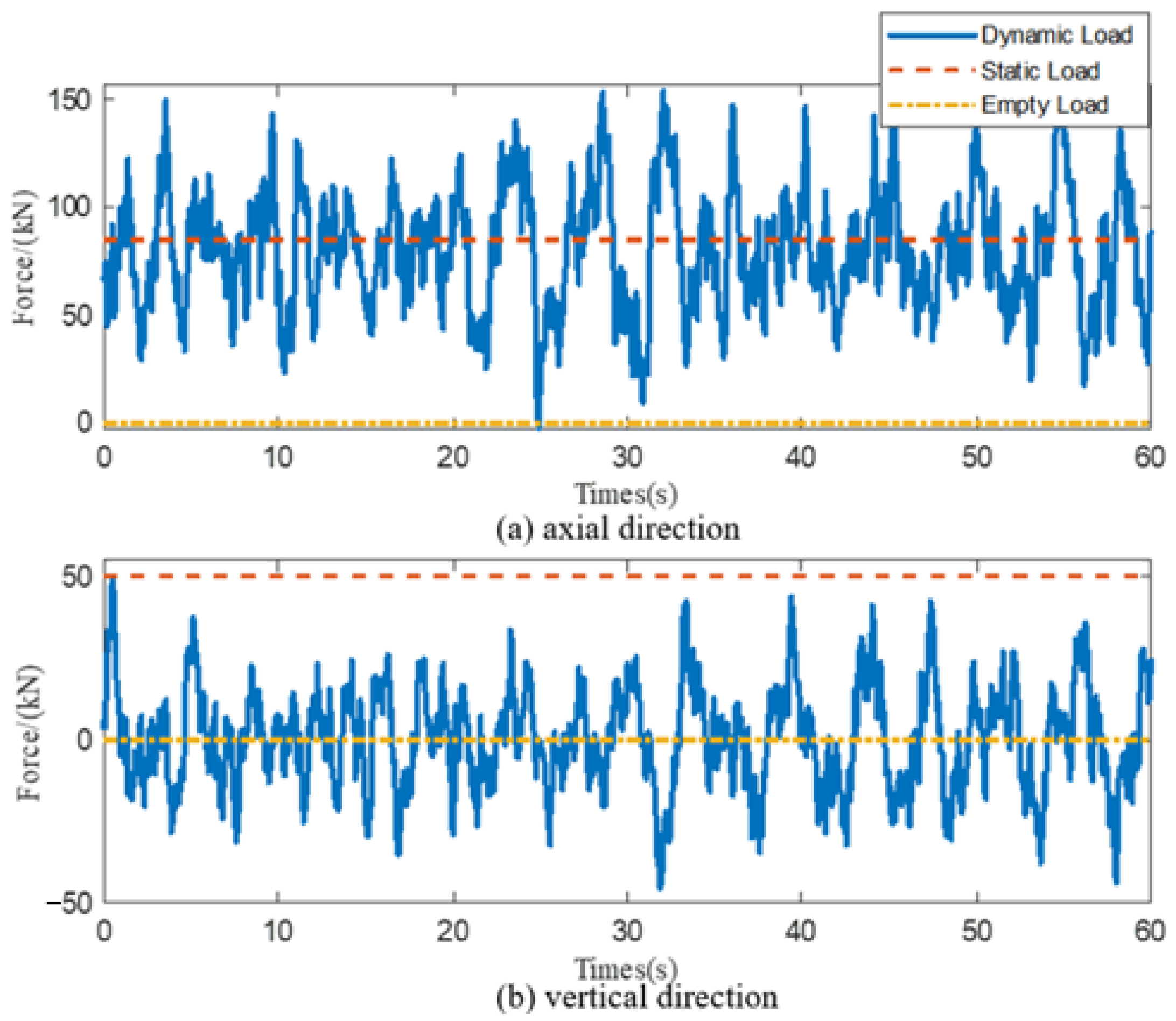
Dynamic load
(Vertical 80 kN with 0.2–20 Hz;
axial 40 kN with 0.2–20 Hz)
3691215
Table 4. Experiment results of the proposed DSTLN methods.
Target
Domain
1200 rpm1500 rpm1800 rpm2100 rpmVariable Speed
0 →2100 → 0 rpm
Source
Domain
Empty
Load
Static
Load
Dynamic
Load
Empty
Load
Static
Load
Dynamic
Load
Empty
Load
Static
Load
Dynamic
Load
Empty
Load
Static
Load
Dynamic
Load
Empty
Load
Static
Load
Dynamic
Load
123456789101112131415
1200
rpm
Empty Load1-99.55%
±0.40
99.17%
±0.28
99.83%
±0.14
98.28%
±1.31
98.55%
±0.41
98.82%
±0.44
97.66%
±0.24
98.29%
±0.34
99.76%
±0.24
98.38%
±0.44
98.39%
±0.28
91.79%
±1.84
86.67%
±2.42
87.38%
±3.73
Static
Load
299.83%
±0.13
-99.78%
±0.12
99.5%
±0.38
99.92%
±0.04
99.67%
±0.26
99.32%
±0.54
98.42%
±0.25
98.13%
±0.76
98.73%
±0.36
98.83%
±0.15
97.29%
±0.45
92.33%
±2.39
92.38%
±3.65
67.42%
±5.36
Dynamic
Load
399.88%
±0.14
99.38%
±0.82
-99.92%
±0.06
99.92%
±0.08
99.96%
±0.04
99.36%
±0.86
98.16%
±0.43
98.79%
±0.34
98.39%
±0.80
97.67%
±1.42
97.88%
±1.18
90.88%
±3.58
93.58%
±1.39
88.54%
±4.28
1500
rpm
Empty Load498.38%
±0.82
99.71%
±0.26
99.88%
±0.10
-99.38%
±0.82
99.96%
±0.02
99.48%
±0.72
98.25%
±0.26
98.25%
±0.36
98.96%
±0.42
97.63%
±0.92
97.58%
±0.84
91.71%
±3.82
86.38%
±4.27
88.38%
±5.36
Static
Load
598.96%
±0.06
99.43%
±0.42
99.68%
±0.21
99.38%
±0.82
-99.88%
±0.08
99.83
±0.14
99.63%
±0.
99.75%
±0.26
99.96%
±0.02
99.71%
±0.28
99.54%
±0.36
91.63%
±2.24
94.83%
±2.18
66.75%
±7.24
Dynamic
Load
698.29%
±0.15
98.45%
±0.68
98.38%
±0.28
99.38%
±0.82
99.56%
±0.22
-99.38%
±0.22
99.82%
±0.08
99.79%
±0.14
99.52%
±0.32
99.96%
±0.03
99.75%
±0.23
93.38%
±3.06
87.83%
±4.52
93.79%
±3.16
1800
rpm
Empty Load798.96%
±0.02
99.31%
±0.56
98.79%
±0.64
99.02
±0.32
99.22%
±0.56
99.92%
±0.06
-99.79%
±0.19
99.25%
±0.38
99.38%
±0.27
99.5%
±0.42
98.83%
±0.12
91.17%
±4.18
85.83%
±5.17
88.71%
±4.92
Static
Load
897.96%
±0.03
99.83%
±0.14
99.54%
±0.36
98.84
±0.59
99.83%
±0.09
99.74%
±0.26
99.38%
±0.82
-98.92%
±0.94
99.83%
±0.06
99.71%
±0.26
99.54%
±0.32
91.29%
±2.02
88.83%
±3.28
88.42%
±5.28
Dynamic Load998.38%
±0.44
98.18%
±0.38
98.23%
±0.62
98.91%
±0.39
98.87%
±0.92
99.21%
±0.48
99.48%
±0.36
99.54%
±0.21
-99.82%
±0.10
99.96%
±0.03
99.92%
±0.04
94.83%
±2.14
90.83%
±2.18
94.88%
±3.14
2100
rpm
Empty Load1098.56%
±0.29
99.12%
±0.35
98.89%
±0.22
99.12%
±0.71
99.67%
±0.26
99.96%
±0.02
99.96%
±0.04
99.79%
±0.18
99.38%
±0.36
-99.75%
±0.16
99.04%
±0.72
91.42%
±3.29
87.88%
±3.48
90.33%
±3.28
Static
Load
1198.88%
±0.30
99.02%
±0.58
99.22%
±0.49
98.87
±0.72
98.62
±0.38
99.88%
±0.10
99.83%
±0.12
99.54%
±0.34
99.54%
±0.38
99.92%
±0.26
-99.71%
±0.26
89.63%
±3.16
92.54%
±2.39
90.38%
±3.66
Dynamic
Load
1298.32%
±0.35
98.43%
±0.58
98.38%
±0.69
99.25%
±0.52
98.89%
±0.42
98.82%
±0.68
98.94%
±0.59
99.10%
±0.38
99.34%
±0.25
99.72%
±0.28
99.88%
±0.06
-95.25%
±3.48
95.25%
±1.36
94.5%
±2.40
Variable
Speed
0→2100→0
rpm
Empty Load1399.64%
±0.24
99.45%
±0.25
99.68%
±0.36
99.24%
±0.52
99.79%
±0.16
99.88%
±0.07
99.13%
±0.69
99.88%
±0.09
100%
±0
100%
±0
99.33%
±0.35
99.75%
±0.16
-95.25%
±3.48
94.88%
±2.06
Static
Load
1499.88%
±0.13
99.25%
±0.36
99.38%
±0.29
99.12%
±0.46
99.27%
±0.38
99.24%
±0.32
99.92%
±0.04
99.28%
±0.52
99.96%
±0.08
99.35%
±0.26
99.92%
±0.06
99.88%
±0.10
97.88%
±1.36
-94.79%
±2.42
Dynamic
Load
1599.96%
±0.02
99.97%
±0.03
99.96%
±0.05
99.98%
±0.06
99.92%
±0.04
99.91%
±0.08
99.96%
±0.04
99.95%
±0.05
99.94%
±0.07
99.96%
±0.02
99.93%
±0.05
99.96%
±0.03
98.79%
±0.53
97.5%
±1.16
-
Disclaimer/Publisher’s Note: The statements, opinions and data contained in all publications are solely those of the individual author(s) and contributor(s) and not of MDPI and/or the editor(s). MDPI and/or the editor(s) disclaim responsibility for any injury to people or property resulting from any ideas, methods, instructions or products referred to in the content.

