Optimal Design of Double-Pole Magnetization BLDC Motor and Comparison with Single-Pole Magnetization BLDC Motor in Terms of Electromagnetic Performance

 ,
, 
Abstract
:1. Introduction
2. Initial Double-Pole Magnetization BLDC Motor
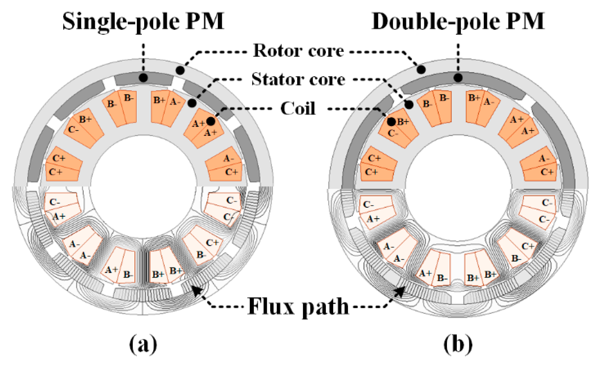
2.1. Analysis Model
2.2. Pole Separation Space
2.3. PM Offset
3. Optimal Design
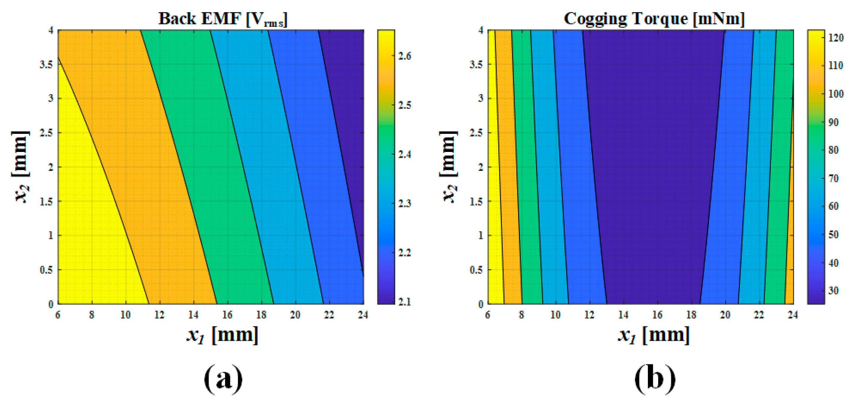
3.1. CCD
3.2. Multiple Response Optimal Method
4. Experimental Verification and Discussion
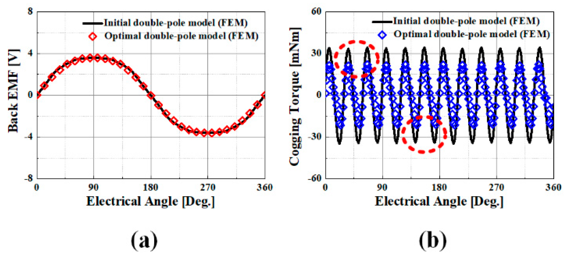
4.1. Experimental Verification
4.2. Discussion
5. Conclusions
Author Contributions
Funding
Institutional Review Board Statement
Informed Consent Statement
Data Availability Statement
Conflicts of Interest
References
- Kim, S.-H. Electric Motor Control: DC, AC, and BLDC Motors, 2nd ed.; D.B. Info: Seoul, Korea, 2017; pp. 114–119. [Google Scholar]
- Damiano, A.; Floris, A.; Fois, G.; Marongiu, I.; Porru, M.; Serpi, A. Design of a High-Speed Ferrite-Based Brushless DC Machine for Electric Vehicles. IEEE Trans. Ind. Appl. 2017, 53, 4279–4287. [Google Scholar] [CrossRef]
- Bianchi, N.; Bolognani, S.; Luise, F. Analysis and Design of aPM Brushless Motor for High-Speed Operations. IEEE Trans. Energy Convers. 2014, 20, 629–637. [Google Scholar] [CrossRef]
- Jang, S.-M.; Cho, H.-W.; Choi, S.-K. Design and Analysis of a High-Speed Brushless DC Motor for Centrifugal Compressor. IEEE Trans. Magn. 2007, 43, 2573–2575. [Google Scholar] [CrossRef]
- Shin, H.-S.; Jang, G.-H.; Choi, J.-Y. Quasi-3D Electromagnetic Analysis and Experimental Verification of Multi-Pole Magnetization BLDC Motor. AIP Adv. 2020, 10, 015218. [Google Scholar] [CrossRef]
- Mellor, P.; Wrobel, R. Optimization of a Multipolar Permanent-Magnet Rotor Comprising Two Arc Segments per Pole. IEEE Trans. Magn. 2007, 43, 942–951. [Google Scholar] [CrossRef]
- Przybylski, M. Multi-Pole Magnetization of Magnets of High Density Magnetic Energy. In Proceedings of the XLIII International Symposium on Electrical Machines SME 2007, Poznan, Poland, 2–5 July 2007. [Google Scholar]
- Hur, J.; Jung, I.-S.; Sung, H.-G.; Park, S.-S. Performance Analysis of a Brushless DC Motor Due to Magnetization Distribution in a Continuous Ring Magnet. J. Appl. Phys. 2003, 93, 8778–8780. [Google Scholar] [CrossRef]
- Karbowiak, M.; Kapelski, D.; Jankowski, B.; Przybylski, M.; Ślusarek, B. The Application of Multi-Pole Bonded Magnets in Electric Motors. Zesz. Probl. Masz. Elektr. 2011, 93, 49–52. [Google Scholar]
- Nguyen, V.-T.; Lu, T.-F. Analytical Expression of the Magnetic Field Created by a Permanent Magnet with Diametrical Magnetization. Prog. Electromagn. Res. C 2018, 87, 163–174. [Google Scholar] [CrossRef] [Green Version]
- Ponce, E.-A.; Leeb, S.-B. A 3-D Field Solution for Axially Polarized Multi-Pole Ring Permanent Magnets and Its Application in Position Measurement. IEEE Trans. Magn. 2020, 56, 8000309. [Google Scholar] [CrossRef]
- Vadde, K.; Syrotiuk, V.; Montgomery, D. Optimizing Protocol Interaction Using Response Surface Methodology. IEEE Trans. Mob. Comput. 2006, 5, 627–639. [Google Scholar] [CrossRef]
- Hendershot, J.; Miller, T. Design of Brushless Permanent-Magnet Motors, 2nd ed.; Motor Design Books LLC: Oxford, UK, 1994; pp. 157–163. [Google Scholar]
- Lee, S.-B. Design of Experiments Based on Minitab Examples; Eretec: Gunpo, Korea, 2017; pp. 342–353. [Google Scholar]
- Si, J.; Zhao, S.; Feng, H.; Cao, R.; Hu, Y. Multi-Objective Optimization of Surface-Mounted and Interior Permanent Magnet Synchronous Motor Based on Taguchi Method and Response Surface Method. IEEE Chin. J. Electr. Eng. 2019, 4, 67–79. [Google Scholar] [CrossRef]
- Woo, D.-K.; Lim, D.-K.; Yeo, H.-K.; Ro, J.-S.; Jung, H.-K. A 2-D Finite-Element Analysis for a Permanent Magnet Synchronous Motor Taking an Overhang Effect into Consideration. IEEE Trans. Magn. 2013, 49, 4894–4899. [Google Scholar] [CrossRef]
- Koo, M.-M.; Choi, J.-Y.; Park, Y.-S.; Jang, S.-M. Influence of Rotor Overhang Variation on Generating Performance of Axial Flux Permanent Magnet Machine Based on 3-D Analytical Method. IEEE Trans. Magn. 2014, 50, 8205905. [Google Scholar] [CrossRef]
- Hanselman, D. Brushless Motors: Magnetic Design, Performances, and Control of Brushless DC and Permanent Magnet Synchronous Motors; E-Man Press: Orono, ME, USA, 2012; pp. 108–111. [Google Scholar]


| Item | Single-Pole Model | Initial Double-Pole Model |
|---|---|---|
| Diameter of outer/inner rotor | 155.6/125.8 mm | |
| Diameter of outer/inner stator | 124.3/64 mm 16 mm | |
| Stack length | ||
| PM thickness/offset | 7/1 mm | |
| PM embrace | 0.82 | 0.91 |
| Magnet Type | Ferrite |
|---|---|
| Remanence | 0.4689 T |
| Coercivity | −340,000 A/m |
| Item | Single-Pole Model | Initial Double-Pole Model |
|---|---|---|
| Back EMF | 2.79 Vrms | 2.76 Vrms |
| Cogging torque | 53 mNm | 69 mNm |
| Point | Order | ||
|---|---|---|---|
| Central point | 1 | 15 | 2 |
| Factorial point | 2 | 10 | 1 |
| 3 | 20 | 1 | |
| 4 | 10 | 3 | |
| 5 | 20 | 3 | |
| Axial point | 6 | 7.93 | 2 |
| 7 | 22.07 | 2 | |
| 8 | 15 | 0.59 | |
| 9 | 15 | 3.41 |
| Response Value | ||||
|---|---|---|---|---|
| Back EMF () | 2.8372 | 7.853e−3 | −0.03091 | −7.455e−4 |
| Cogging torque () | 312.562 | −35.0899 | −2.76561 | 1.11455 |
| Item | Unit | Objective | Lower Limit | Target Value | Upper Limit |
|---|---|---|---|---|---|
| Back EMF () | Vrms | Target value | 2.6 | 2.7 | 2.8 |
| Cogging torque () | mNm | Minimization | 30 | 50 |
| Design Variable | Initial Model | Optimal Model |
|---|---|---|
| Pole separation space () | 15 mm | 14.3 mm |
| PM offset () | 2 mm | 3.1 mm |
| Parameters | Experiment | FEM (Error Ratio) |
|---|---|---|
| Back EMF [Vrms] | 2.77 | 2.79 (0.71%) |
| Cogging torque [mNm] | 50 | 53 (5.66%) |
| DC terminal voltage [V] | 13.5 | 13.5 |
| Line current [Arms] | 58.17 | 58.96 (1.34%) |
| Torque [Nm] | 2.38 | 2.42 (1.65%) |
| Speed [rpm] | 2594 | 2670 (2.85%) |
| Efficiency [%] | 90.91 | 92.28 (1.48%) |
| Parameters | Initial Model (Error Ratio) | Optimal Model (Error Ratio) |
|---|---|---|
| Back EMF [Vrms] | 2.76 (0.36%) | 2.78 (0.36%) |
| Cogging torque [mNm] | 69 (27.54%) | 44 (13.54%) |
| DC terminal voltage [V] | 13.5 | 13.5 |
| Line current [Arms] | 59.15 (1.66%) | 58.96 (1.34%) |
| Torque [Nm] | 2.43 (2.06%) | 2.43 (2.06%) |
| Speed [rpm] | 2679 (3.17%) | 2678 (3.14%) |
| Efficiency [%] | 92.18 (1.37%) | 92.19 (1.38%) |
Publisher’s Note: MDPI stays neutral with regard to jurisdictional claims in published maps and institutional affiliations. |
© 2021 by the authors. Licensee MDPI, Basel, Switzerland. This article is an open access article distributed under the terms and conditions of the Creative Commons Attribution (CC BY) license (http://creativecommons.org/licenses/by/4.0/).
Share and Cite
Shin, H.-S.; Jang, G.-H.; Jung, K.-H.; Cho, S.-K.; Choi, J.-Y.; Shin, H.-J. Optimal Design of Double-Pole Magnetization BLDC Motor and Comparison with Single-Pole Magnetization BLDC Motor in Terms of Electromagnetic Performance. Machines 2021, 9, 18. https://0-doi-org.brum.beds.ac.uk/10.3390/machines9010018
Shin H-S, Jang G-H, Jung K-H, Cho S-K, Choi J-Y, Shin H-J. Optimal Design of Double-Pole Magnetization BLDC Motor and Comparison with Single-Pole Magnetization BLDC Motor in Terms of Electromagnetic Performance. Machines. 2021; 9(1):18. https://0-doi-org.brum.beds.ac.uk/10.3390/machines9010018
Chicago/Turabian StyleShin, Hyo-Seob, Gang-Hyeon Jang, Kyung-Hun Jung, Seong-Kook Cho, Jang-Young Choi, and Hyeon-Jae Shin. 2021. "Optimal Design of Double-Pole Magnetization BLDC Motor and Comparison with Single-Pole Magnetization BLDC Motor in Terms of Electromagnetic Performance" Machines 9, no. 1: 18. https://0-doi-org.brum.beds.ac.uk/10.3390/machines9010018