A Collision Avoidance Strategy for Redundant Manipulators in Dynamically Variable Environments: On-Line Perturbations of Off-Line Generated Trajectories ^†

Abstract

In this work, a comprehensive control strategy for obstacle avoidance in redundant manipulation is presented, consisting of a combination of off-line path planning algorithms with on-line motion control. Path planning allows the avoidance of fixed obstacles detected before the start of the robot’s motion; it is based on the potential fields method combined with a smoothing process realized by means of interpolation with Bezier curves. The on-line motion control is designed to compensate for the motion of the obstacles and to avoid collisions along the kinematic chain of the manipulator; it is realized by means of a velocity control law based on the null space method for redundancy control. A new term is introduced in the control law to take into account the speed of the obstacles as well as their position. Simulations on a simplified planar case are presented to assess the validity of the algorithms and to estimate the computational effort in order to verify the transferability of our approach to a real system.

1. Introduction

Collaborative robotics has recently gained an important role in industrial production, attracting the attention of researchers. Collaborative robotics refers to the cooperation between humans and robots to accomplish a certain task in a shared workspace; it is the meeting point between flexibility and productivity needs and is made possible by the use of advanced safety technologies. In addition, collaborative robotics involves specific techniques to control robots working in a dynamic environment that is not known in advance and to modify planned motions to avoid collisions with humans and obstacles [1].

When a manipulator is intended to work in environments in which potential obstacles may interfere with its motion, a certain degree of redundancy is useful for its kinematic reconfiguration [2]. Thus, thanks to its dexterity, a redundant manipulator is the best candidate in collision avoidance applications. Moreover, redundancy can also be exploited with standard manipulators if some of the degrees of freedom of the end-effector—e.g., the orientation angles—can be kept free during motion.

An overall control strategy for a manipulator working in a dynamic environment can be conceived as the combination of the following:

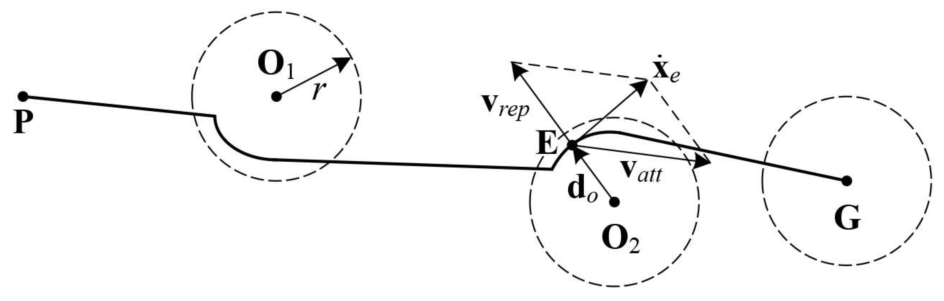
• An off-line path planning algorithm, which plans the trajectory of the robot end-effector taking into account the possible presence of disturbing obstacles, modifying the path based on the positions of the obstacles before the motion starts;
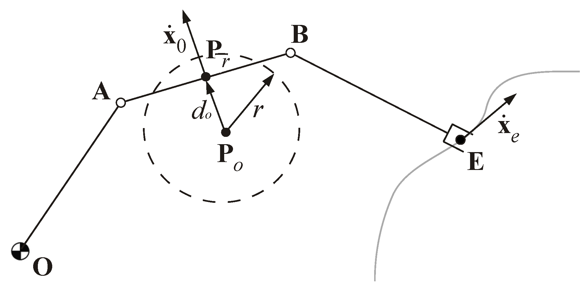
• An on-line motion control algorithm, which controls the robot in real-time to compensate for obstacles that are moving or new obstacles entering the workspace, also avoiding collisions between obstacles and points belonging to the kinematic chain of the manipulator.

Several methods dealing with motion planning for obstacle avoidance are available in the literature [3]. As an example, the obstacle avoidance problem is solved by the configuration space motion method in [4], whereas a distance-propagating dynamic system is proposed in [5] for dynamic environments. Furthermore, a model predictive control is presented in [6] with a BIT (Batch Informed Trees) method that improves the path point connections, whereas in [7], collision-free paths are generated using an RRT (Rapidly-Exploring Random Trees) algorithm. Moreover, a very common approach to path planning is to define artificial potential fields, which drive the robot to the target inside the workspace [8,9,10,11]. The result of the potential fields is a set of forces that are attractive toward the goal and repulsive from the obstacle regions. Typically, such forces are associated with velocities applied to the end-effector of the manipulator; then, the trajectory can be obtained by numerical integration. An example of a path planning strategy based on potential fields method is proposed in [9], where a saturation function for the attractive velocity is introduced in order to avoid oscillations around the goal point; furthermore, for the repulsive velocity, a spring–damper system is used to eliminate noise in proximity of the obstacles. A further problem in optimal path planning for automation and robotics is the generation of smooth trajectories, as highlighted in [3,12]: an optimal algorithm for trajectory generation must guarantee smoothness in terms of position and velocity in order to be implemented in the controller of a real system. That is the case, for example, with CPP (Coverage Path Planning) techniques, typically used for service mobile robots, where algorithms are able to generate smooth paths, avoiding sharp turns and thus reducing accelerations and decelerations [13,14].

The same principle of repulsive velocities generated by obstacles can be used in order to avoid collisions between obstacles and control points along the kinematic chain of the manipulator: in addition to the motion imposed on the end-effector, a repulsive velocity vector can be applied to the point of the robot that is closer to one of the obstacles, adding a task to the control system [15,16,17,18,19]. Specifying some studies, a comprehensive work can be found in [2], where a kinematic control for on-line obstacle avoidance in a redundant manipulator is proposed and an approximated and computationally efficient solution for the pseudoinverse is used to manage the redundancy of the manipulator; in [5], a grid-based distance-propagating dynamic system is adopted, where penalty functions are used to generate safety margins around the obstacles.

Overview and Contribution

This study proposes a control strategy for obstacle avoidance in redundant manipulators using a combination of off-line path planning and an on-line motion control algorithms. Starting from the research background provided by the aforementioned studies, a combination and synthesis of the best candidate methods has been already presented by authors in [20]. In this work, some improvements are given, introducing two main novel contributions:

• Off-line path planning is combined with a smoothing interpolation based on Bezier curves in order to avoid sharp edges and high accelerations [21,22,23,24,25,26,27];
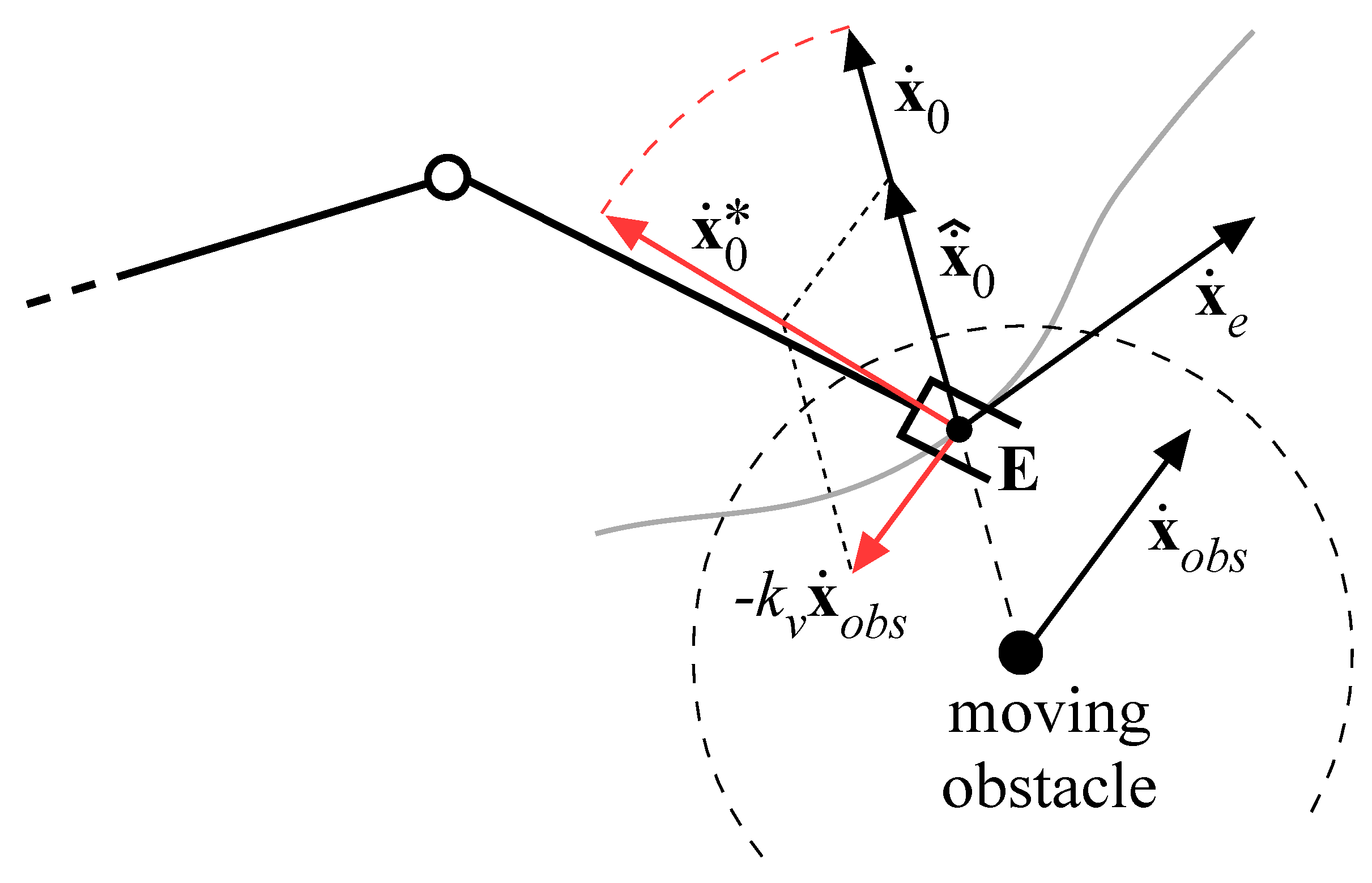
• Regarding collision avoidance control, an additional term depending on the velocity of an obstacle is introduced, previewing its next position in order to plan the optimal correction of the trajectory.

Algorithms are tested by simulation on a simplified case; i.e., a planar manipulator with three revolute joints (3R) in a two degree-of-freedom (2-DOF) task space. The results confirm the effectiveness of the method and give an insight into the required computational effort. The advantages due to the novel improvements introduced in the algorithms can be summarized as follows:

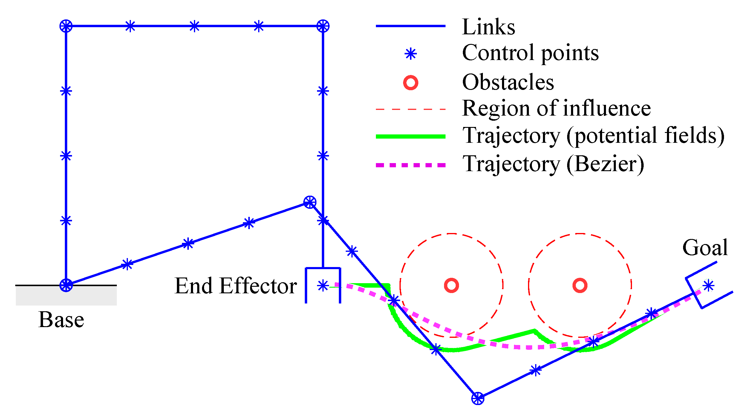
• The capability of generating smooth trajectories with a closed-form interpolation procedure, which requires a very low computational time;
• The reinforcement of the motion control strategy in the case of moving obstacles, without a significant increase of the computational effort.

The remainder of the paper is organized as follows: Section 2 describes the trajectory path planning algorithm, where the artificial potential fields method and a smoothing procedure that exploits Bezier curves are combined; Section 3 discusses the on-line motion control, including the direct and inverse kinematics of the manipulator, the obstacle avoidance strategy based on the null space method and the introduction of an additional term that improves the ability of the robot to avoid moving obstacles; Section 4 discusses and compares the performance of the algorithm in different conditions; and a preview of future work and concluding remarks are given in Section 5 and Section 6, respectively.

2. Off-Line Path Planning

A trajectory planning algorithm is needed at first in order to define the motion ${\mathbf{x}}_e\left(t\right)$ to be assigned to the end-effector to reach a target position and avoid the obstacles that are inside the workspace before the motion of the manipulator starts. The strategy proposed in [20] is based on the definition of potential fields that generate repulsive or attractive velocity components, defined as ${\mathbf{v}}_{rep}$ and ${\mathbf{v}}_{att}$, respectively, which drive the end-effector $\mathbf{E}$ following the minimum potential path towards the goal. As shown in Figure 1, $\mathbf{P}$ is the initial position of the end-effector, $\mathbf{G}$ is the goal and ${\mathbf{O}}_i$ represents the obstacles, with their area of influence outlined by the radius $\mathit{r}$. Moreover, ${\mathbf{d}}_O=\mathbf{E}-{\mathbf{O}}_i$ and ${\mathbf{d}}_G=\mathbf{G}-\mathbf{E}$. Equation (1) defines attractive and repulsive velocities as

$${\mathbf{v}}_{att}=\{\begin{array}{cc}{v}_{att}{\displaystyle \frac{{\mathbf{d}}_G}{r}}\hfill & \hspace{1em}{d}_G<r\hfill \\ v_{att}{\widehat{\mathbf{d}}}_G\hfill & \hspace{1em}{d}_G\ge r\hfill \end{array}\hspace{1em}\hspace{1em}{\mathbf{v}}_{rep}=\{\begin{array}{cc}{\displaystyle \frac{v_{rep}}{d_O}}\left({\displaystyle \frac{1}{d_O}}-{\displaystyle \frac{1}{r}}\right)\nabla d_O\hfill & d_O<r\hfill \\ 0\hfill & d_O\ge r\hfill \end{array}$$

(1)

The end-effector trajectory can be found by the numerical integration of the resulting velocity:

$${\dot{\mathbf{x}}}_e={\mathbf{v}}_{rep}+{\mathbf{v}}_{att}{\mathbf{x}}_e(t+\mathrm{d}t)={\mathbf{x}}_e\left(t\right)+{\dot{\mathbf{x}}}_e\left(t\right)\mathrm{d}t$$

(2)

Then, an interpolation with a fifth-order polynomial allows the generation of a motion law.

A path resulting from Equations (1) and (2) is typically characterized by short-radius curves and sharp corners that may cause high accelerations and vibration problems, as shown in the example of Figure 2: the robot in the initial and final configurations is sketched in blue, while obstacles are the red circles and their region of influence is delimited by dashed circles; the green curve is the path obtained by means of the potential fields method.

An improvement of the presented algorithm can be obtained by avoiding its critical issues due to sharp corners by using a smoother kind of curve—i.e., a Bezier curve—which interpolates the original curve with a best-fit approach. The new algorithm considers three possible orders of Bezier curves, from three to five, with an increasing level of detail/complexity and computational effort. Given $n+1$ points ${\mathbf{P}}_0, {\mathbf{P}}_1, \cdots ,{\mathbf{P}}_n$, where n is the power of the Bezeir curve, the latter is defined as

$$\mathbf{B}\left(s\right)=\sum _{i=0}^n\left(\genfrac{}{}{0pt}{}{n}{i}\right){\mathbf{P}}_i{(1-s)}^{n-i}{s}^i,s\in [0,1]$$

(3)

Without any loss of generality, let us consider a third-order Bezier curve:

$$\mathbf{B}={\mathbf{P}}_0{(1-s)}^3+3{\mathbf{P}}_{1}s{(1-s)}^2+3{\mathbf{P}}_2{s}^2(1-s)+{\mathbf{P}}_3{s}^3$$

(4)

where the points ${\mathbf{P}}_0$ and ${\mathbf{P}}_3$ are coincident with the starting and goal points, respectively; the fitting procedure seeks for points ${\mathbf{P}}_1$ and ${\mathbf{P}}_2$, generating the curve $\mathbf{B}$ that best approximates the original one with a least-square metric. A closed-form solution to the problem can be found by manipulating Equation (4) as follows:

$${\mathbf{B}}^T=\left[\begin{array}{cc}1-s^3& s^3\end{array}\right]{\left[\begin{array}{cc}{\mathbf{P}}_0& {\mathbf{P}}_3\end{array}\right]}^T+\left[\begin{array}{cc}3s(1-s^2)& 3s^2(1-s)\end{array}\right]{\left[\begin{array}{cc}{\mathbf{P}}_1& {\mathbf{P}}_2\end{array}\right]}^T$$

(5)

If the curvilinear abscissa s is discretized in m samples, the trajectory ${\mathbf{x}}_e$ becomes a set of m points. Thus, Equation (5) can be written m times for the points ${\mathbf{B}}_j, j=1\cdots m$, assuming the form

$$\mathbf{N}={\mathbf{S}}_1{\mathbf{C}}_1+{\mathbf{S}}_2{\mathbf{C}}_2$$

(6)

where:

$$\mathbf{N}={\left[\begin{array}{c}{\mathbf{B}}_1 \cdots {\mathbf{B}}_m\end{array}\right]}^T{\mathbf{S}}_1=\left[\begin{array}{cc}1-s_1^3& s_1^3\\ ⋮& ⋮\\ 1-s_m^3& s_m^3\end{array}\right]{\mathbf{S}}_2=\left[\begin{array}{cc}3s_1(1-s_1^2)& 3s_1^2(1-s_1)\\ ⋮& ⋮\\ 3s_m(1-s_m^2)& 3s_m^2(1-s_m)\end{array}\right]$$

(7)

$${\mathbf{C}}_1={\left[\begin{array}{cc}{\mathbf{P}}_0& {\mathbf{P}}_3\end{array}\right]}^T{\mathbf{C}}_2={\left[\begin{array}{cc}{\mathbf{P}}_1& {\mathbf{P}}_2\end{array}\right]}^T$$

(8)

A closed-form solution for the optimal set of coefficients ${\mathbf{C}}_2$ can be easily found by manipulating Equation (6) and substituting the matrix $\mathbf{N}$ with the analogous matrix $\mathbf{X}$ that is built with the points belonging to the trajectory ${\mathbf{x}}_e$ found with the potential field algorithm:

$${\mathbf{C}}_2={{\mathbf{S}}_2}^{†}(\mathbf{X}-{\mathbf{S}}_1{\mathbf{C}}_1)\mathbf{X}={\left[\begin{array}{c}{\mathbf{x}}_{e,1} \cdots {\mathbf{x}}_{e,m}\end{array}\right]}^T$$

(9)

where † represents the pseudoinverse operator according to the Moore–Penrose definition. The result of the smoothing procedure is shown in Figure 2 by the magenta curve. Furthermore, Figure 3 gives a comparison between third and fourth-order polynomials: in the first case, the interpolation is less accurate, violating the influence area of an obstacle, whereas in the second case, the fitting is better, but the trajectory is less smooth; higher orders will result in overly sharp curvatures and high computational times and thus they are not suitable for this purpose.

3. On-Line Motion Control

A simplified planar case is analyzed in this work in order to assess the functionality of the algorithms: a 2D motion in the Cartesian space $\mathbf{x}={[x y]}^T$ is planned using the 3R manipulator shown in Figure 4, which is controlled in the joint space $\mathbf{q}={[{\theta }_1 {\theta }_2 {\theta }_3]}^T$. Thus, the kinematics of the manipulator has a redundant degree of freedom with respect to the task. Each link has the same length, L. Besides the end-effector $\mathbf{E}$, a total of 12 control points belonging to the kinematic chain characterizes the manipulator; three of them are in correspondence with the joints $\mathbf{O}$, $\mathbf{A}$ and $\mathbf{B}$, and the others are equally spaced along the links (e.g., ${\mathbf{A}}_1,{\mathbf{A}}_2,{\mathbf{A}}_3$).

The forward kinematics of the manipulator can be described by

$$\mathbf{x}=\mathbf{f}\left(\mathbf{q}\right)$$

(10)

$$\dot{\mathbf{x}}=\mathbf{J}\left(\mathbf{q}\right)\dot{\mathbf{q}}$$

(11)

where $\mathbf{f}$ represents the expression of the position forward kinematics and $\mathbf{J}$ is the $(2\times 3)$ Jacobian matrix. Due to redundancy, the inverse position kinematics problem is not defined in a closed form, but it can be defined by the following differential formulation:

$$\dot{\mathbf{q}}={\mathbf{J}}^{†}\dot{\mathbf{x}}+\mathbf{N}{\dot{\mathbf{q}}}_0$$

(12)

$$\mathbf{q}(t+\mathrm{d}t)=\mathbf{q}\left(t\right)+\dot{\mathbf{q}}\left(t\right)\mathrm{d}t$$

(13)

where ${\dot{\mathbf{q}}}_0$ is the joint null space velocity, whose effect is to generate internal motions, leaving the pose of the end-effector unchanged; ${\mathbf{J}}^{†}$ = ${\mathbf{J}}^{\mathbf{T}}{\left({\mathbf{JJ}}^{\mathbf{T}}\right)}^{-1}$ is the pseudoinverse of the Jacobian matrix $\mathbf{J}$; $\mathbf{N}$ = $\mathbf{I}-{\mathbf{J}}^{†}\mathbf{J}$ is the projection into the null space of $\mathbf{J}$.

In addition to the basic control law, an obstacle avoidance strategy is introduced: inspired by the null space methods for the control of redundant manipulators, an additional velocity vector is assigned to the control point of the robot which is the closest to one of the obstacles within the workspace, so that the control point can move away form the obstacle, while the motion of the end-effector is not affected. In more detail, referring to Figure 5, the pair of points ${\mathbf{P}}_r$ and ${\mathbf{P}}_o$ at the minimum distance $d_o$ is identified at each time step. The area of influence of the obstacles is delimited by the radius r. If, at a certain time step during the motion, the condition $d_o<r$ is verified, a repulsive velocity ${\dot{\mathbf{x}}}_0$ is imposed to the relative control point along the direction of $d_o$. As the manipulator is characterized by one redundant DOF, only one repulsive velocity vector can be assigned at each time step; thus, the point to which it is assigned may change over time with the criterion of the minimum distance from one of the obstacles. This point can be also the end-effector: besides the velocity vector ${\dot{\mathbf{x}}}_e$ assigned by the off-line path planning in order to describe the desired trajectory, the repulsive velocity vector can be applied to $\mathbf{E}$, modifying its trajectory, if the position of an obstacle changes from its initial state or a new obstacle enters the workspace, interfering with the motion of $\mathbf{E}$. In this case, the position of the end-effector drifts from the originally planned trajectory, originating a position error that must be recovered by introducing a proportional corrective term in the control law, as typically done in Closed Loops Inverse Kinematics (CLIK) algorithms [28].

In terms of equations, the expressions given in Equations (14) and (15) must be imposed in order to assign the two velocity tasks described above:

$$\mathbf{J}\dot{\mathbf{q}}={\dot{\mathbf{x}}}_e$$

(14)

$${\mathbf{J}}_0\dot{\mathbf{q}}={\dot{\mathbf{x}}}_e$$

(15)

where ${\mathbf{J}}_0$ represents the Jacobian matrix associated to the velocity of the point ${\mathbf{P}}_r$.

Thus, Equation (12) can be modified in [29,30]:

$$\dot{\mathbf{q}}={\mathbf{J}}^{†}{\dot{\mathbf{x}}}_c+\left({\mathbf{J}}_0{\mathbf{N}}^{†}\right)({\dot{\mathbf{x}}}_0-{\mathbf{J}}_0{\mathbf{J}}^{†}{\dot{\mathbf{x}}}_e)$$

(16)

where ${\dot{\mathbf{x}}}_c=\dot{{\mathbf{x}}_e}+k\mathbf{e}$ is the corrected end-effector velocity, k the positive gain and $\mathbf{e}$ is the position error between the desired position ${\mathbf{x}}_e$ and the actual position $\mathbf{x}$. The first term of Equation (16) guarantees the exact velocity of the end effector with a minimum joint speed. The second term drives the motion of the point ${\mathbf{P}}_r$ of the robot, satisfying the collision avoidance additional task.

The Equation (16) can be further simplified: as the obstacle avoidance strategy requires only the motion in the direction of the line connecting the most critical point of the robot with the closest point on the obstacle, this is a one-dimensional constraint. Therefore, it is possible to define the Jacobian ${\mathbf{J}}_0$ as proposed by [2]:

$${\mathbf{J}}_{d0}={\widehat{\mathbf{d}}}^T{\mathbf{J}}_0$$

(17)

where $\widehat{\mathbf{d}}={\mathbf{d}}_o/\left|\right|{\mathbf{d}}_o\left|\right|$ is the direction along which the repulsive velocity is applied. The dimension of the matrix ${\mathbf{J}}_{d0}$ is $(1\times n)$, and velocities ${\dot{\mathbf{x}}}_0$ and ${\mathbf{J}}_0{\mathbf{J}}^{†}{\dot{\mathbf{x}}}_e$ become scalars. It was proved in [2] that, with this approach, the calculation of the term ${\left({\mathbf{J}}_0\mathbf{N}\right)}^{†}$ in Equation (16) is faster and the system has fewer singularities. With few passages, the final form of the solution for $\dot{\mathbf{q}}$ is

$$\dot{\mathbf{q}}={\mathbf{J}}^{†}{\dot{\mathbf{x}}}_c+\mathbf{N}{\mathbf{J}}_{d0}{\left({\mathbf{J}}_{d0}\mathbf{N}{\mathbf{J}}_{d0}^T\right)}^{-1}({\dot{x}}_0-{\mathbf{J}}_{d0}{\mathbf{J}}^{†}{\dot{\mathbf{x}}}_e)$$

(18)

The choice of ${\dot{x}}_0$ is a critical point of the algorithm. The proposed strategy is to change ${\dot{x}}_0$ according to the distance from the obstacle. To avoid discontinuity and give smoothness to the motion, two weighting coefficients, $a_h$ and $a_v$, are introduced:

$${\dot{x}}_0=a_v{v}_{rep}$$

(19)

$$\dot{\mathbf{q}}={\mathbf{J}}^{†}{\dot{\mathbf{x}}}_c+a_h\mathbf{N}{\mathbf{J}}_{d0}{\left({\mathbf{J}}_{d0}\mathbf{N}{\mathbf{J}}_{d0}^T\right)}^{-1}(a_v{v}_{rep}-{\mathbf{J}}_{d0}{\mathbf{J}}^{†}{\dot{\mathbf{x}}}_e)$$

(20)

Thus, a nominal repulsive velocity $v_{rep}$ is modulated by $a_v$ as a function of the distance $d_o$, whereas $a_h$ acts with a weight that balances the effect of the homogeneous solution (related to the collision avoidance) with respect to the total.

In more detail, let r be the control distance that defines the area of influence of an obstacle, $r_{min}$ be the distance under which no action is possible and $r_m$ be an intermediate critical distance between $r_{min}$ and r. No influence of the obstacle is desired if $d_o>r$, while the algorithm fails (the robot stops) if $d_o<r_{min}$. Between these limits, the weighting coefficients must vary continuously from 0 to 1, as shown in Figure 6 and according to the following equations:

$$a_v=\{\begin{array}{cc}{\left({\displaystyle \frac{d_o-r_m}{r_{min}-r_m}}\right)}^2\hfill & d_o<r_m\hfill \\ 0\hfill & d_o\ge r_m\hfill \end{array}$$

(21)

$$a_h=\{\begin{array}{ccc}1\hfill & \hfill & d_o\le r_m\hfill \\ {\displaystyle \frac{1}{2}}\left[1-cos\left(\pi {\displaystyle \frac{d_o-r_m}{r-r_m}}\right)\right]\hfill & \hfill & r_m<d_o<r\hfill \\ 0\hfill & \hfill & d_o\ge r\hfill \end{array}$$

(22)

A further novel contribution is introduced to improve the ability of the algorithm to avoid moving obstacles: it is reasonable that not only the position but also the velocity of an obstacle should influence the control of the robot. As an example, if the end-effector moves toward an obstacle moving with an orthogonal velocity, it is preferable to modify the trajectory of the end-effector, pushing it in a direction opposite to the obstacle velocity. Thus, if the end-effector is the control point closest to the obstacle, the repulsive velocity vector ${\dot{\mathbf{x}}}_0$ is modified as follows:

$$\begin{array}{c}\hfill {\dot{\mathbf{x}}}_0^{*}={\dot{\mathbf{x}}}_0\frac{{\widehat{x}}_0-k_v{\dot{\mathbf{x}}}_{obs}}{\sqrt{1+{k_v}^2{\dot{\mathbf{x}}}_{obs}^2}}\end{array}$$

(23)

where, as described in Figure 7, ${\dot{\mathbf{x}}}_{obs}$ is the obstacle velocity, ${\dot{\mathbf{x}}}_0$ is the repulsive velocity along the direction of $d_0$, $k_v$ is a gain term and ${\dot{\mathbf{x}}}_0^{*}$ is the modified repulsive velocity applied to the end-effector in combination with the planned velocity ${\dot{\mathbf{x}}}_e$. The effect is that the direction of the repulsive velocity is modified, whereas its magnitude does not change; furthermore, for $k_v=0$, the effect vanishes.

4. Results

The algorithms presented in the previous sections were tested by simulations over a wide range of conditions. In this section, two examples are shown: the first one investigated the avoidance of two fixed obstacles, while the second one considered two moving obstacles. In both cases, a common set of parameters were used, which are summarized in

Table 1. Parameter values used for simulations.

$\mathit{L} \left[\mathbf{m}\right]$	$\mathit{r} \left[\mathbf{m}\right]$	${\mathit{r}}_{\mathit{m}} \left[\mathbf{m}\right]$	${\mathit{r}}_{\mathbf{min}} \left[\mathbf{m}\right]$	${\mathit{v}}_{\mathbf{rep}} [\mathbf{m}/\mathbf{s}]$	${\mathit{v}}_{\mathbf{att}} [\mathbf{m}/\mathbf{s}]$	K	$\mathit{T} \left[\mathbf{s}\right]$	$\mathbf{d}\mathit{t} \left[\mathbf{s}\right]$
1	0.25	0.225	0.2	10	5	20	1	${10}^{-3}$

.

Figure 8 shows six steps of the motion of the 3R robot when two fixed obstacles were interposed between the starting and the goal points. In this case, the off-line planner was able to find a smooth curve (third-order Bezier curve) to accomplish the task; then, the on-line control acted to avoid collisions with internal points of the robot. For example, at $t=0.45 \mathrm{s}$ the second-last control point, immediately upstream of the end-effector, entered the area of influence of the obstacle, but the control reacted by imposing a repulsive velocity to that point, as clearly visible also in Figure 9 where ${\theta }_2$ and ${\theta }_3$ angles are subject to a sudden rotation.

The fast change in joint angles may result in a peak of the velocity profile, which must be compared with the limits of the manipulator. Considering the previous example, the resulting joint speed law is plotted in Figure 10a. As the times and dimensions of the manipulator were arbitrary chosen in the simulation, absolute values of joint speeds may not have been realistic, which would make it unhelpful to compare them to the hypothetical speed limits of a real machine. Nevertheless, we can imagine that a joint speed limit was fixed at $15 \mathrm{rad}/\mathrm{s}$ so that the peak related to the third joint would not have admissible and the speed would reach saturation approximately at $t=0.45 \mathrm{s}$ (Figure 10b). In this case, the end-effector would be subjected to a further deviation due to the speed saturation, as shown in Figure 10c, where the black curve is related to the simulation without saturation, whereas the blue curve corresponds to the velocity law of Figure 10b. Nevertheless, the end-effector would still be able to reach the goal thanks to the term in the control law which is proportional to the position error $\mathbf{e}$.

The second simulated case, shown in Figure 11, considered two obstacles initially external to the trajectory of the manipulator but that moved toward the path of the robot with orthogonal (opposite) velocities. Thus, approximately at $t=0.45 \mathrm{s}$, the control modified the trajectory of the end-effector in order to avoid the collision. However, at $t=0.7 \mathrm{s}$ the obstacles stimulated the control in two opposite ways, and the robot became stuck in its position, failing the task. This criticality is even more evident in Figure 12, where the curves of the joint angles can be seen to be unstable due to the fast counteracting effects of the control.

A solution to this kind of problem can be found by introducing the modified repulsive velocity defined in Equation (23): Figure 13 plots the motion of the manipulator in the same scenario as Figure 11 (where the gain $k_v$ was null), with the only difference being a positive gain $k_v=100$, thus activating the dependency of the repulsive velocity on the velocity of the obstacle. In this case, when the first interference occurred at $t=0.45 \mathrm{s}$ the control pushed the end-effector downwards, opposite to the velocity of the first obstacle, and vice versa when the second obstacle was reached at approximately $t=0.55 \mathrm{s}$. Then, as the position of the end-effector drifted from the planned trajectory due to the action of the control for collision avoidance, the position error was recovered by the action of the proportional term $k\mathbf{e}$ in Equation (16) until the final position was correctly reached. In this case, the velocity profile shown in Figure 14 demonstrates the stability of the control strategy in completing the task.

A further issue assessed by the simulations was the computational effort required for the execution of the algorithms. In all cases, a standard laptop was used (i7 CPU @1.8 GHz, 16 GB RAM). For the execution of the off-line path planning algorithm with the third-order Bezier curve, the average computational time was in the order of ${10}^{-2} \mathrm{s}$, depending on the number of obstacles, and this may reach ${10}^{-1} \mathrm{s}$ using the fourth-order curve. The on-line motion control was able to run in all cases with a cycle time in the order of ${10}^{-4} \mathrm{s}$, thus being comparable with rates typically used in the communication between external controllers and the main controllers of robots. An increase of computational time is expected when extending the algorithm to the 3D space, but the use of better performing hardware hints at the applicability of our approach to real systems.

5. Discussion

In a industrial environment, a robot, while performing its task, could meet obstacles which could represent both humans (a point may represent the distal extremity a part of the body, such as an arm, a hand, etc.) and objects interfering with the path and the kinematic chain of the manipulator. The objects could be, for example, furniture or mechanical equipment left inadvertently inside the workspace. As an example, consider a pick and place application in which a robot performs its task assisted by a human operator who may accidentally interfere with the operation by placing an arm along the path of the robot. In this case, the robot must be able to recognize and avoid a dangerous situation. Thus, it becomes necessary to apply a strategy to control the robot, even in the presence of unknown obstacles. Considering this kind of scenario, future work will include the implementation of the proposed algorithms on a 7 degrees of freedom manipulator (KUKA LBR iiwa), extending the control to a full mobility problem in 3D [31]. The final objective will be to transfer the control framework to a real system, now under construction in the laboratory, where the robot will be equipped with a vision system composed of multiple 3D cameras that is able to acquire information regarding the surrounding environment and extrapolate the positions of objects and humans inside the workspace [32,33,34,35]. The collision-free HRC system will be tested in the laboratory, and the transferability of the algorithms to a real system will be finally experimentally validated.

6. Conclusions

In this paper, an obstacle avoidance strategy for robots moving in dynamically varying environments was presented and verified by simulation. Two novel contributions to the algorithms have been introduced: first, the trajectory planned by the potential field method is smoothed using a best-fit interpolation with Bezier curves; second, a modified repulsive velocity for the end-effector was introduced in order to consider also the velocity of the obstacles, improving the avoidance ability in dynamic environments. Simulations confirmed the effectiveness of the control strategy and gave an estimation of the computational effort required to execute the algorithms, which is in line with the typical requirements of robot controllers and can be improved by using high-performing hardware.

References

1. Pedrocchi, N.; Vicentini, F.; Matteo, M.; Tosatti, L.M. Safe human-robot cooperation in an industrial environment. Int. J. Adv. Robot. Syst. 2013, 10, 27. [Google Scholar] [CrossRef]
2. Zlajpah, L.; Nemec, B. Kinematic control algorithms for on-line obstacle avoidance for redundant manipulators. In Proceedings of the IEEE/RSJ International Conference on Intelligent Robots and Systems, Lausanne, Switzerland, 30 September–4 October 2002; Volume 2, pp. 1898–1903. [Google Scholar]
3. Gasparetto, A.; Boscariol, P.; Lanzutti, A.; Vidoni, R. Path planning and trajectory planning algorithms: A general overview. In Motion and Operation Planning of Robotic Systems; Springer: Berlin/Heidelberg, Germany, 2015; pp. 3–27. [Google Scholar]
4. Han, B.; Luo, X.; Luo, Q.; Zhao, Y.; Lin, B. Research on Obstacle Avoidance Motion Planning Technology of 6-DOF Manipulator. In Proceedings of the International Conference on Geometry and Graphics, São Paulo, Brazil, 2 December 2020; Springer: Cham, Switzerland, 2021; pp. 604–614. [Google Scholar]
5. Willms, A.R.; Yang, S.X. Real-time robot path planning via a distance-propagating dynamic system with obstacle clearance. IEEE Trans. Syst. Man Cybern. Part B (Cybern.) 2008, 38, 884–893. [Google Scholar] [CrossRef] [PubMed] [Green Version]
6. Xu, P.; Wang, N.; Dai, S.L.; Zuo, L. Motion Planning for Mobile Robot with Modified BIT* and MPC. Appl. Sci. 2021, 11, 426. [Google Scholar] [CrossRef]
7. Wang, J.; Liu, S.; Zhang, B.; Yu, C. Manipulation Planning with Soft Constraints by Randomized Exploration of the Composite Configuration Space. Int. J. Control. Autom. Syst. 2021, 19, 1–12. [Google Scholar]
8. Jung, J.H.; Kim, D.H. Local Path Planning of a Mobile Robot Using a Novel Grid-Based Potential Method. Int. J. Fuzzy Log. Intell. Syst. 2020, 20, 26–34. [Google Scholar] [CrossRef]
9. Xu, X.; Hu, Y.; Zhai, J.; Li, L.; Guo, P. A novel non-collision trajectory planning algorithm based on velocity potential field for robotic manipulator. Int. J. Adv. Robot. Syst. 2018, 15, 1729881418787075. [Google Scholar] [CrossRef] [Green Version]
10. Borenstein, J.; Koren, Y. Real-time obstacle avoidance for fast mobile robots. IEEE Trans. Syst. Man, Cybern. 1989, 19, 1179–1187. [Google Scholar] [CrossRef] [Green Version]
11. Lee, K.; Choi, D.; Kim, D. Potential Fields-Aided Motion Planning for Quadcopters in Three-Dimensional Dynamic Environments. In Proceedings of the AIAA Scitech 2021 Forum, Reston, VA, USA, 19–21 January 2021; p. 1410. [Google Scholar]
12. Gasparetto, A.; Zanotto, V. A new method for smooth trajectory planning of robot manipulators. Mech. Mach. Theory 2007, 42, 455–471. [Google Scholar] [CrossRef]
13. Hassan, M.; Liu, D.; Chen, X. Squircular-CPP: A Smooth Coverage Path Planning Algorithm based on Squircular Fitting and Spiral Path. In Proceedings of the 2020 IEEE/ASME International Conference on Advanced Intelligent Mechatronics (AIM), Boston, MA, USA, 6–9 July 2020; pp. 1075–1081. [Google Scholar] [CrossRef]
14. Lakshmanan, A.K.; Mohan, R.E.; Ramalingam, B.; Le, A.V.; Veerajagadeshwar, P.; Tiwari, K.; Ilyas, M. Complete coverage path planning using reinforcement learning for tetromino based cleaning and maintenance robot. Autom. Constr. 2020, 112, 103078. [Google Scholar] [CrossRef]
15. Maciejewski, A.A.; Klein, C.A. Obstacle avoidance for kinematically redundant manipulators in dynamically varying environments. Int. J. Robot. Res. 1985, 4, 109–117. [Google Scholar] [CrossRef] [Green Version]
16. Safeea, M.; Béarée, R.; Neto, P. Collision Avoidance of Redundant Robotic Manipulators Using Newton’s Method. J. Intell. Robot. Syst. 2020, 1–9. [Google Scholar] [CrossRef] [Green Version]
17. Zhang, H.; Jin, H.; Liu, Z.; Liu, Y.; Zhu, Y.; Zhao, J. Real-time kinematic control for redundant manipulators in a time-varying environment: Multiple-dynamic obstacle avoidance and fast tracking of a moving object. IEEE Trans. Ind. Informatics 2019, 16, 28–41. [Google Scholar] [CrossRef]
18. Mazzanti, M.; Cristalli, C.; Gagliardini, L.; Carbonari, L.; Lattanzi, L.; Massa, D. A Novel Trajectory Generation Algorithm for Robot Manipulators with Online Adaptation and Singularity Management. In Proceedings of the 2019 IEEE 28th International Symposium on Industrial Electronics (ISIE), Vancouver, BC, Canada, 12–14 June 2019; pp. 1115–1120. [Google Scholar]
19. Abhishek, T.S.; Schilberg, D.; Doss, A.S.A. Obstacle Avoidance Algorithms: A Review. In Proceedings of the IOP Conference Series: Materials Science and Engineering, Tangerang, Indonesia, 18–20 November 2020; IOP Publishing: Bristol, UK, 2021; Volume 1012, p. 012052. [Google Scholar]
20. Scoccia, C.; Palmieri, G.; Palpacelli, M.C.; Callegari, M. Real-Time Strategy for Obstacle Avoidance in Redundant Manipulators. In Proceedings of the International Conference of IFToMM, Naples, Italy, 9–11 September 2020; Springer: Berlin/Heidelberg, Germany, 2020; pp. 278–285. [Google Scholar]
21. Lattarulo, R.; González, L.; Perez, J. Real-Time Trajectory Planning Method Based On N-Order Curve Optimization. In Proceedings of the 2020 24th International Conference on System Theory, Control and Computing (ICSTCC), Sinaia, Romania, 8–10 October 2020; pp. 751–756. [Google Scholar]
22. Chen, L.; Qin, D.; Xu, X.; Cai, Y.; Xie, J. A path and velocity planning method for lane changing collision avoidance of intelligent vehicle based on cubic 3-D Bezier curve. Adv. Eng. Softw. 2019, 132, 65–73. [Google Scholar] [CrossRef]
23. Kawabata, K.; Ma, L.; Xue, J.; Zhu, C.; Zheng, N. A path generation for automated vehicle based on Bezier curve and via-points. Robot. Auton. Syst. 2015, 74, 243–252. [Google Scholar] [CrossRef]
24. Corinaldi, D.; Carbonari, L.; Callegari, M. Optimal Motion Planning for Fast Pointing Tasks With Spherical Parallel Manipulators. IEEE Robot. Autom. Lett. 2018, 3, 735–741. [Google Scholar] [CrossRef]
25. Corinaldi, D.; Callegari, M.; Angeles, J. Singularity-free path-planning of dexterous pointing tasks for a class of spherical parallel mechanisms. Mech. Mach. Theory 2018, 128, 47–57. [Google Scholar] [CrossRef]
26. Hsu, T.W.; Liu, J.S. Design of smooth path based on the conversion between η 3 spline and Bezier curve. In Proceedings of the 2020 American Control Conference (ACC), Denver, CO, USA, 1–3 July 2020; pp. 3230–3235. [Google Scholar]
27. Yu, X.; Zhu, W.; Xu, L. Real-time Motion Planning and Trajectory Tracking in Complex Environments based on Bézier Curves and Nonlinear MPC Controller. In Proceedings of the 2020 Chinese Control And Decision Conference (CCDC), Hefei, China, 22–24 August 2020; pp. 1540–1546. [Google Scholar]
28. Melchiorre, M.; Scimmi, L.S.; Pastorelli, S.P.; Mauro, S. Collison Avoidance using Point Cloud Data Fusion from Multiple Depth Sensors: A Practical Approach. In Proceedings of the 2019 23rd International Conference on Mechatronics Technology (ICMT), Salerno, Italy, 23–26 October 2019; pp. 1–6. [Google Scholar]
29. Cefalo, M.; Magrini, E.; Oriolo, G. Sensor-based task-constrained motion planning using model predictive control. IFAC-PapersOnLine 2018, 51, 220–225. [Google Scholar] [CrossRef]
30. Lee, K.K.; Buss, M. Obstacle avoidance for redundant robots using Jacobian transpose method. In Proceedings of the 2007 IEEE/RSJ International Conference on Intelligent Robots and Systems, San Diego, CA, USA, 29 October–2 November 2007; pp. 3509–3514. [Google Scholar]
31. Flacco, F.; Kröger, T.; De Luca, A.; Khatib, O. A depth space approach to human-robot collision avoidance. In Proceedings of the 2012 IEEE International Conference on Robotics and Automation, Saint Paul, MN, USA, 14–18 May 2012; pp. 338–345. [Google Scholar]
32. Dröder, K.; Bobka, P.; Germann, T.; Gabriel, F.; Dietrich, F. A machine learning-enhanced digital twin approach for human-robot-collaboration. Procedia Cirp 2018, 76, 187–192. [Google Scholar] [CrossRef]
33. Rosenstrauch, M.J.; Pannen, T.J.; Krüger, J. Human robot collaboration-using kinect v2 for ISO/TS 15066 speed and separation monitoring. Procedia CIRP 2018, 76, 183–186. [Google Scholar] [CrossRef]
34. Scalera, L.; Giusti, A.; Vidoni, R.; Di Cosmo, V.; Matt, D.T.; Riedl, M. Application of dynamically scaled safety zones based on the ISO/TS 15066:2016 for collaborative robotics. Int. J. Mech. Control 2020, 21, 41–49. [Google Scholar]
35. Bucolo, M.; Buscarino, A.; Fortuna, L.; Gagliano, S. Force Feedback Assistance in Remote Ultrasound Scan Procedures. Energies 2020, 13, 3376. [Google Scholar] [CrossRef]
Figure 1. Potential field for trajectory planning.
Machines 09 00030 g001
Figure 2. Path planning for a planar 3R manipulator and two fixed obstacles.
Machines 09 00030 g002
Figure 3. Trajectory interpolation: comparison between 3rd (a) and 4th (b) order Bezier curves.
Machines 09 00030 g003
Figure 4. Planar 3R manipulator with control points.
Machines 09 00030 g004
Figure 5. Velocity components for the end-effector and the closest control point of the robot.
Machines 09 00030 g005
Figure 6. Weighting coefficients a v and a h as functions of the distance d o .
Machines 09 00030 g006
Figure 7. Modified repulsive velocity.
Machines 09 00030 g007
Figure 8. Example of the avoidance of two fixed obstacles.
Machines 09 00030 g008
Figure 9. Joint rotations for the example of Figure 8.
Machines 09 00030 g009
Figure 10. (a) Joint speeds for the example of Figure 8; (b) joint speeds with saturation limit; (c) comparison between trajectories.
Machines 09 00030 g010
Figure 11. Example of avoidance of two moving obstacles ( k v = 0 ) .
Machines 09 00030 g011
Figure 12. Joint rotations for the example of Figure 11.
Machines 09 00030 g012
Figure 13. Example of avoidance of two moving obstacles ( k v = 100 ) .
Machines 09 00030 g013
Figure 14. Joint rotations for the example of Figure 13.
Machines 09 00030 g014