
Perspectives on SCADA Data Analysis Methods for Multivariate Wind Turbine Power Curve Modeling

Department of Engineering, University of Perugia, 06125 Perugia, Italy
Machines 2021, 9(5), 100; https://0-doi-org.brum.beds.ac.uk/10.3390/machines9050100
Submission received: 13 April 2021
/
Revised: 2 May 2021
/
Accepted: 11 May 2021
/
Published: 13 May 2021
(This article belongs to the Special Issue Condition Monitoring for Non-stationary Rotating Machines)
Abstract
:Wind turbines are rotating machines which are subjected to non-stationary conditions and their power depends non-trivially on ambient conditions and working parameters. Therefore, monitoring the performance of wind turbines is a complicated task because it is critical to construct normal behavior models for the theoretical power which should be extracted. The power curve is the relation between the wind speed and the power and it is widely used to monitor wind turbine performance. Nowadays, it is commonly accepted that a reliable model for the power curve should be customized on the wind turbine and on the site of interest: this has boosted the use of SCADA for data-driven approaches to wind turbine power curve and has therefore stimulated the use of artificial intelligence and applied statistics methods. In this regard, a promising line of research regards multivariate approaches to the wind turbine power curve: these are based on incorporating additional environmental information or working parameters as input variables for the data-driven model, whose output is the produced power. The rationale for a multivariate approach to wind turbine power curve is the potential decrease of the error metrics of the regression: this allows monitoring the performance of the target wind turbine more precisely. On these grounds, in this manuscript, the state-of-the-art is discussed as regards multivariate SCADA data analysis methods for wind turbine power curve modeling and some promising research perspectives are indicated.
1. Introduction
Modern horizontal-axis wind turbines are complex machines which are subjected to non-stationary conditions; therefore, monitoring their performance is a complicated task which has attracted a wide debate in the scientific literature.
Typically, the manufacturer of a wind turbine provides standards for the behavior of the machine, basing on field test in a controlled environment: these are expressed in the form of curves for the thrust coefficient and for the power coefficient. Unfortunately, in real-world applications, the aerodynamics and the machine design are useful only within a certain extent because the environmental conditions to which the wind turbines are subjected can be remarkably different with respect to the reference. Furthermore, there are relevant issues related to the quality of the measurements, because the standard is the use of cup anemometers mounted behind the rotor span and the undisturbed wind speed is estimated through a nacelle transfer function. It is a consolidated evidence that the nacelle transfer function is affected by turbulence intensity, wind shear, atmospheric stability and other environmental factors [1,2].
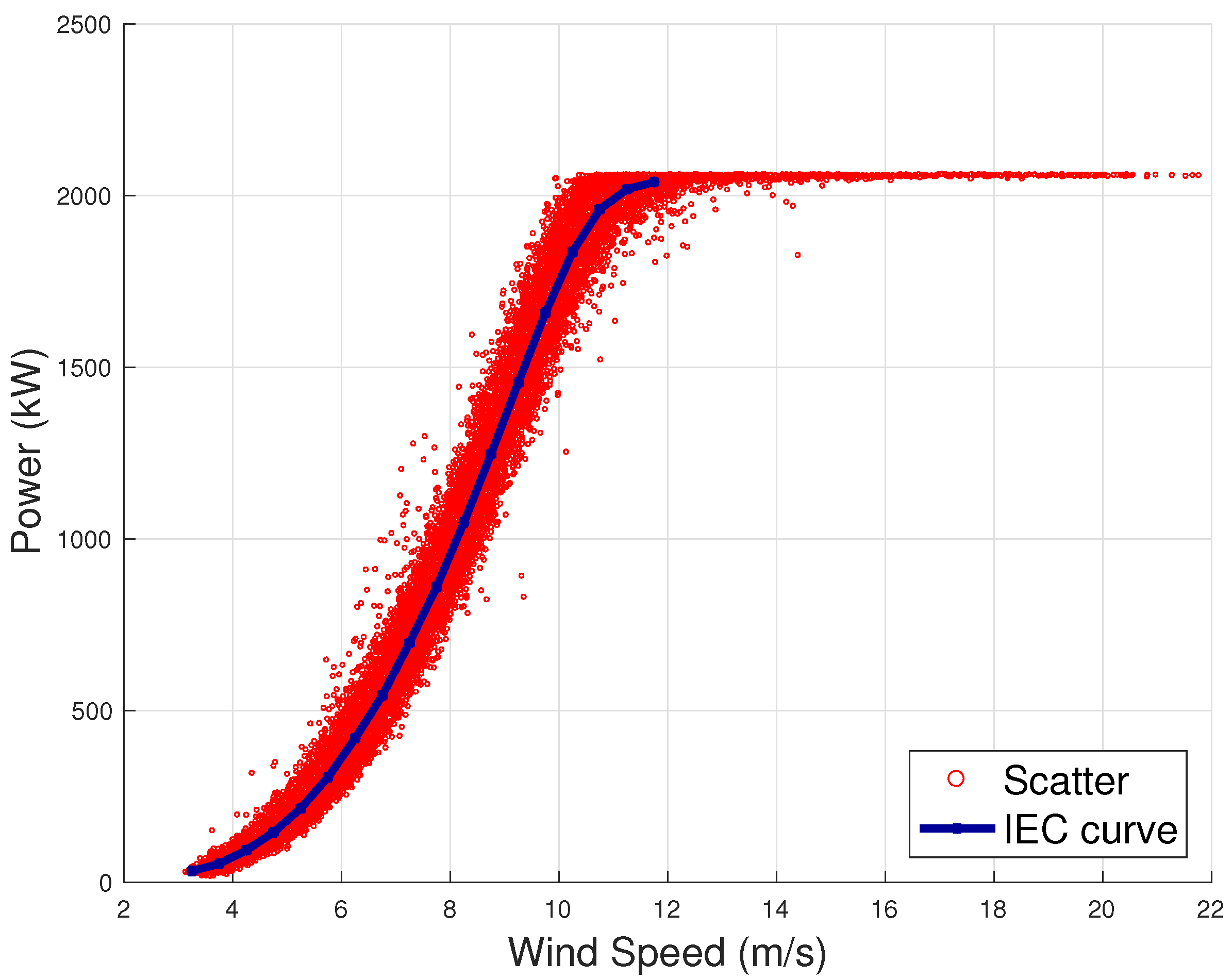
The power curve of a wind turbine is fundamental to understand its performance because it is given by the measured relation between the wind speed and the output power, which can be visualized through a simple two-dimensional scatter plot. The method most commonly employed for visualizing power curves has been codified in the IEC [3] guidelines. These substantially consist of the so called binning method, which is based on averaging the measured power in wind speed intervals of 0.5 or 1 m/s.
Given the ith wind speed bin, the average wind speed for the bin is computed as
and the average power for the bin is computed as
where is the normalized measured wind speed of the jth data set in the ith wind speed bin, is the normalized measured power output of the jth data set in the ith wind speed bin and is the population of the ith wind speed bin. In Figure 1, an example of a power curve of a 2 MW wind turbine from an industrial wind farm (owned by ENGIE Italia) is reported, in the form of scatter plot and of IEC power curve.
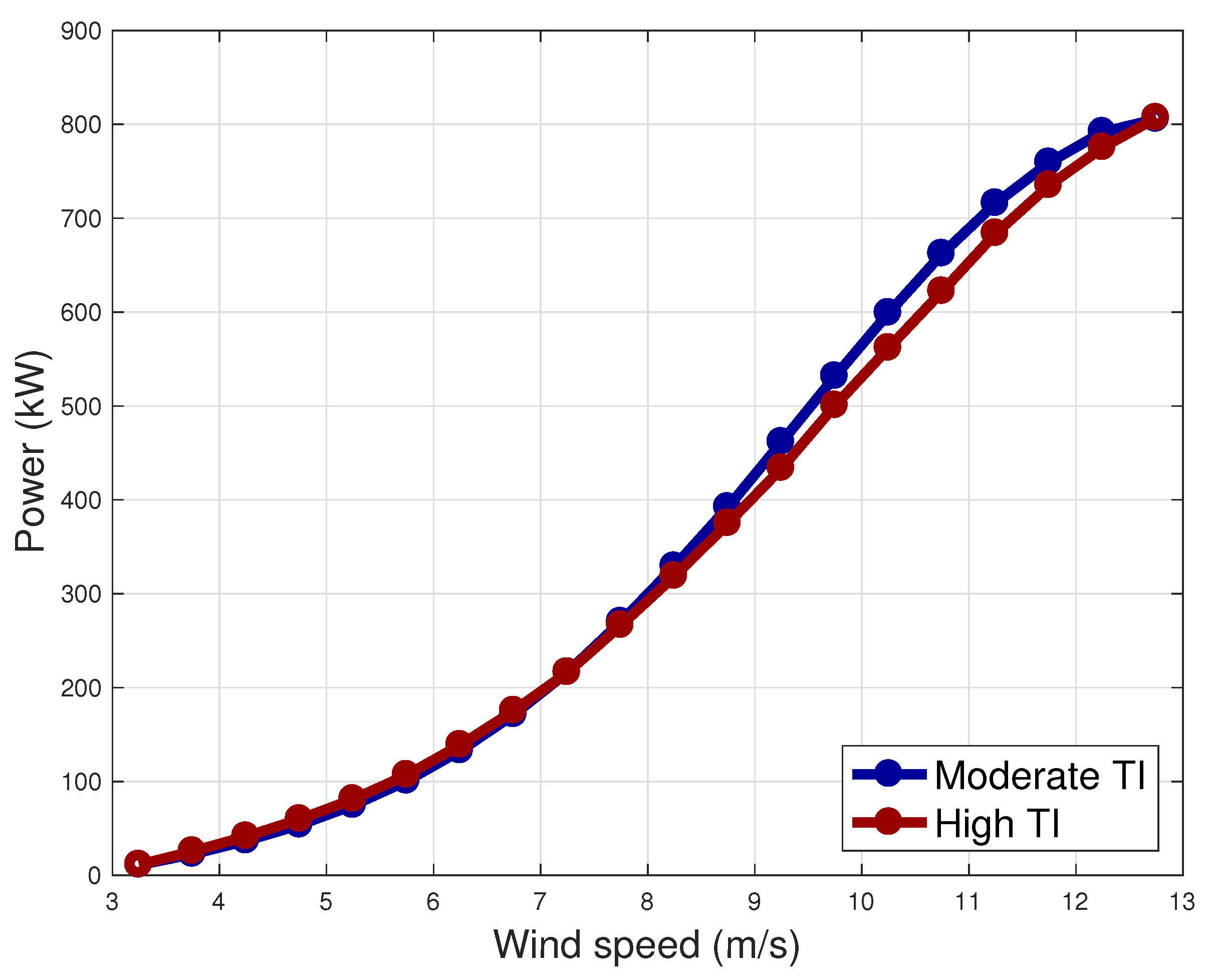
A relevant issue regarding the analysis of power curves through the binning method is that the comparison of the same wind turbine models in different sites is questionable. On the grounds of the above considerations regarding nacelle anemometers, the power curves of two wind turbines of the same model, which are placed in different environments, can appear to be different and it is complicated to argue if this is due to different performance or to uncontrollable environmental effects. This matter of fact is exemplified by Figure 2, where the power curve is reported for two wind turbines of the same model (Vestas V52) which are placed in different environments: one is moderately ( at the order of 8–9 m/s) and one is highly turbulent ( at the order of 8–9 m/s).
Despite this, by the point of view of customization of performance analysis, the power curve obtained through the binning method is a step forward with respect to design specifications, because it is a benchmark which can be constructed for each wind turbine in each site. Therefore, in wind energy practice the attitude has grown to customize the performance monitoring by constructing normal behavior models which refer to a particular wind turbine in a particular site. In this regard, the turning point has been the development and the widespread diffusion of SCADA control systems, storing (typically with ten minutes of sampling time) a vast set of environmental, operational, thermal and electrical measurements. SCADA data represent a powerful information source, but to monitor reliably the performance of wind turbines it is necessary to elaborate the environmental and operational data at disposal and to construct a normal behavior model, i.e., a benchmark for comparing against the measured power.
For this reason, several studies in the literature have been devoted to the improvement of the data-driven regression between wind speed and power. A comprehensive review about wind turbine power curve modeling is given in [4]. Several aspects have been addressed as regards the mismatch between nominal and real-world power curves [5]: the effect of the wind direction [6], in relation to the terrain and wind farm layout, of the wind shear and vertical wind profile [2], or of the turbulence intensity [7]. Currently, it is therefore widely accepted that the power curve of a wind turbine is strongly site-dependent [8].
Despite the above awareness, the most employed approach for the improvement of wind turbine power curve analysis consists of the optimization of the data-driven model [9], using the wind speed (possibly adjusted for taking into account ambient conditions) as input and targeting the power production as output. In the author’s opinion, this approach has an intrinsic limitation because it consists of finding a line of best fit from a two dimensional data points dispersion (as can be appreciated also from the simple example of from Figure 1). The power extracted by a wind turbine for given average wind speed (measured by an anemometer placed behind the rotor center) can vary considerably. For example, if the rotor size increases [10], the wind speed measurement at the center of the rotor might be an insufficient information for quantifying with precision the amount of power which will be extracted. In general, the power of a wind turbine has a multivariate dependence on ambient conditions and working parameters (as, for example, rotor speed and blade pitch), which can be expressed [11] in Equation (3):
In Equation (3), P is the produced power, depending on the rotor radius R, the air density , the wind speed v and the power factor , which depends on the blade pitch angle and the tip-speed ratio (or, in other words, the rotational speed ). Due to environmental effects which are uncontrollable in the absence of further sensors in addition to the SCADA systems, it can happen that a wind turbine responds with a slightly different blade pitch angle or rotational speed to the same average wind speed (measured on 10 min time basis). Therefore, the general idea of multivariate approaches to wind turbine performance monitoring is incorporating further information, in addition to the wind speed, in the normal-behavior model for the power.
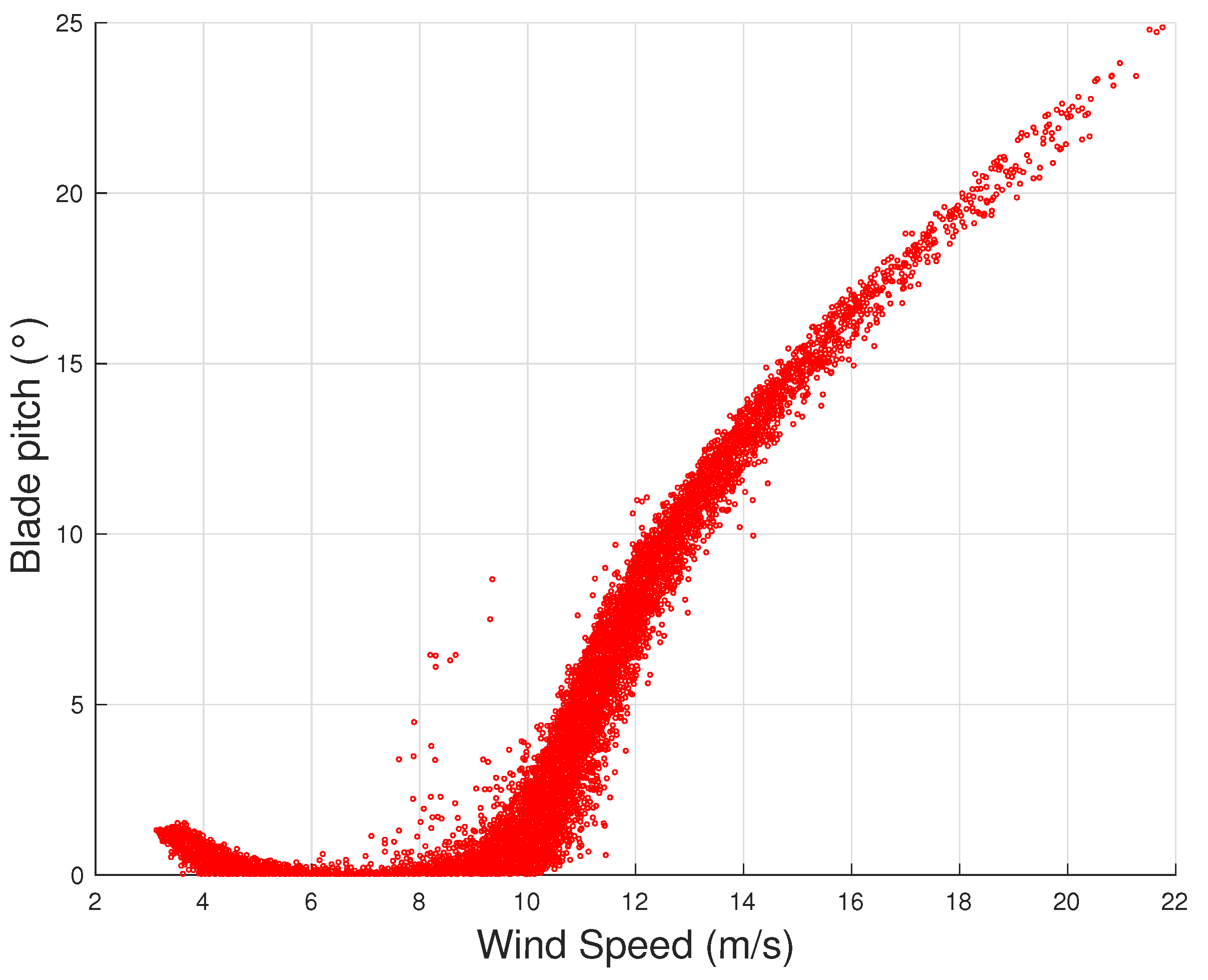
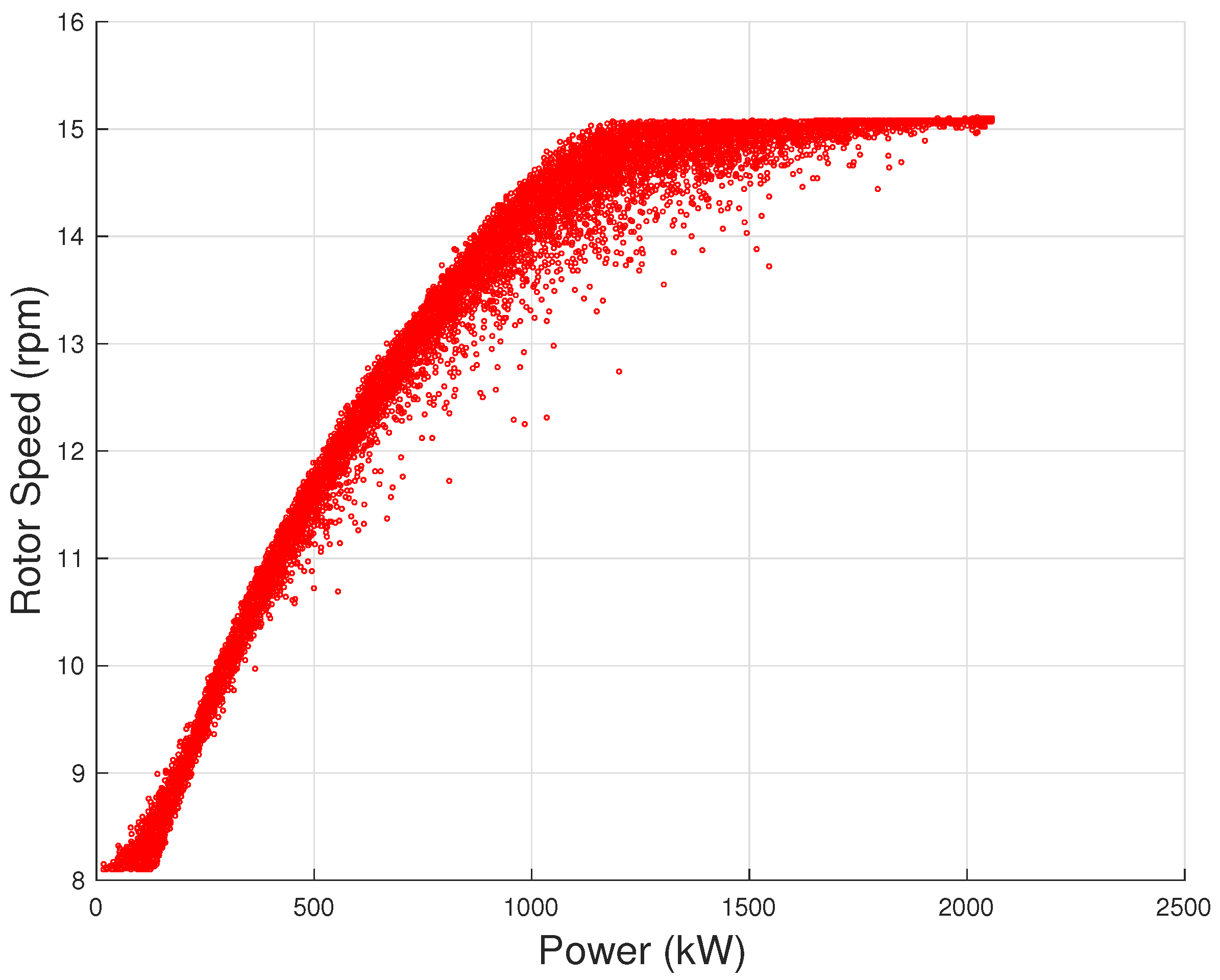
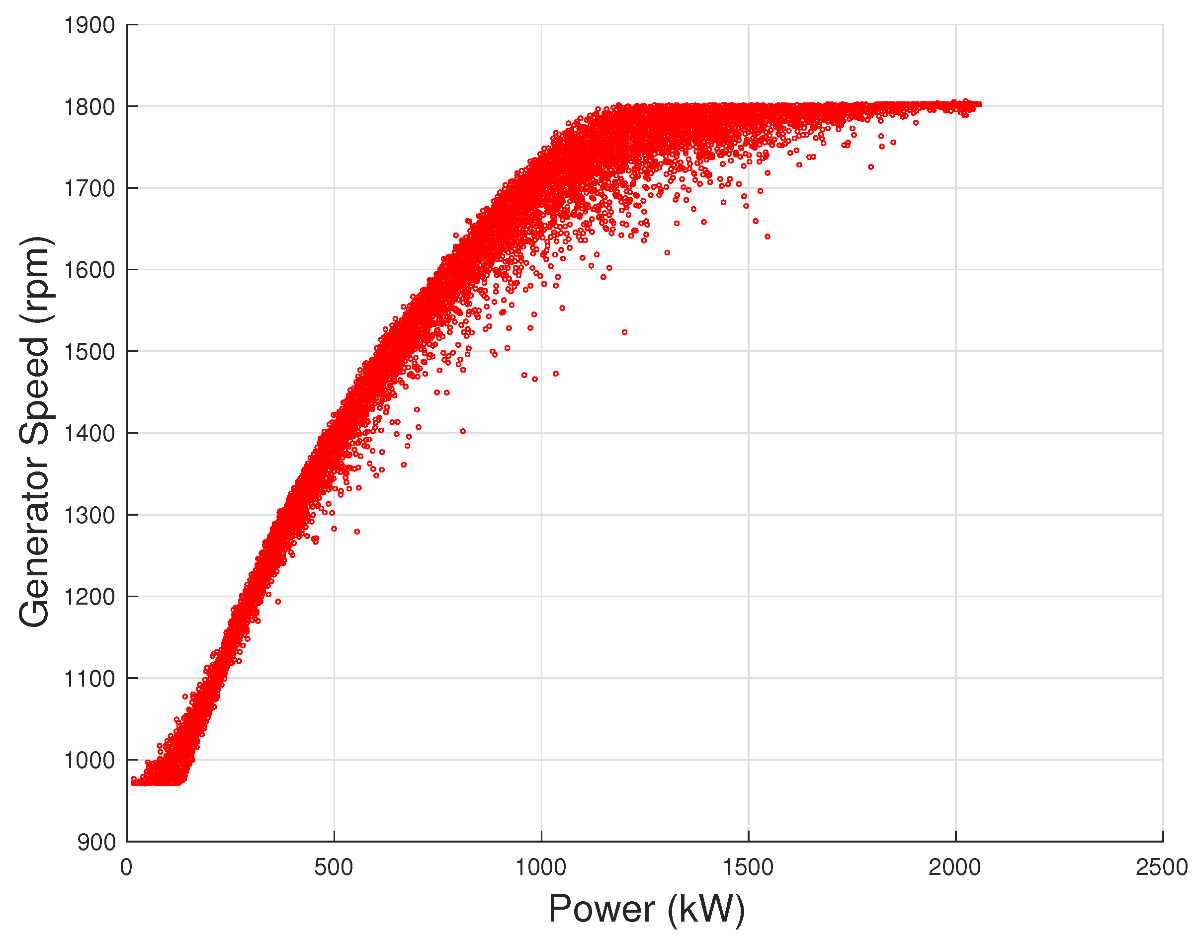
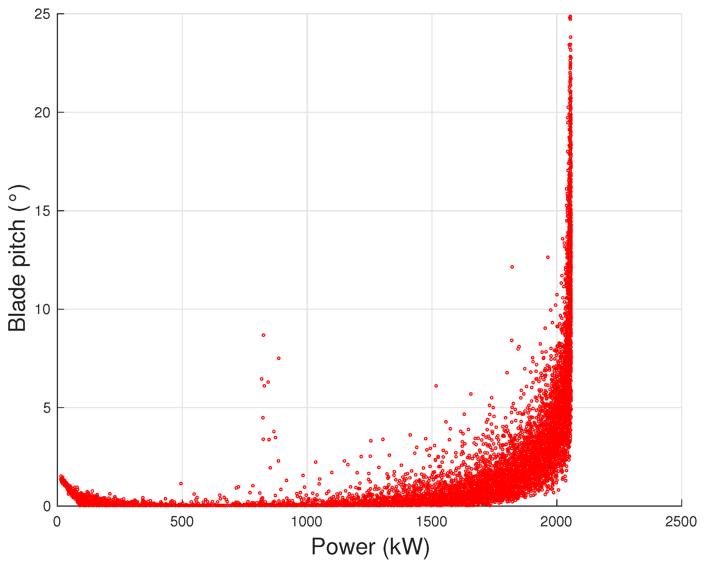
In this regard, it should be mentioned that there are other operation curves, which are instructive for the analysis of wind turbine performance. For example, in [12,13], the wind speed–blade pitch curve of wind turbines (Figure 3) is analyzed using Support Vector Regression and the results are compared against the binning method. In [14], two fundamental operation curves are analyzed through Gaussian process methods, which are the wind speed–blade pitch and the wind speed–rotor speed (Figure 4) curves. Other important operation curves, which have been addressed, for example, in [15,16], are the rotor speed–power (Figure 5), the generator speed–power (Figure 6) and the blade pitch–power curves (Figure 7): examples are reported using the same data set as for Figure 1 (courtesy of ENGIE Italia).
From Figure 3 and Figure 4, it arises that, as the wind intensity increases from cut-in, at first the rotational speed increases and the blade pitch is held practically fixed: in this regime, the wind turbine operates by regulating the rotor speed on the grounds of the torque exerted on the rotor, in order to attain the maximum possible aerodynamic efficiency. For higher wind speed (but below rated power), the logic of the control changes because the rotor speed saturates and the wind turbine operates in partial aerodynamic load, which is regulated by varying the blade pitch. Despite that it is typical that the region from cut-in to rated power is overall indicated as Region 2 of the power curve, it should be noticed that in general these two different control regions can be individuated and it makes sense to distinguish the variable rotor speed with respect to the variable blade pitch control region: for this reason, in [15,16], the nomenclature Region 2 and Region 2 is adopted.
On the grounds of Equation (3) and Figure 3, Figure 4, Figure 5, Figure 6 and Figure 7, it therefore arises intuitively that knowing, for example, the blade pitch and the rotor speed in addition to the wind speed could be helpful for predicting how much power the wind turbine should extract. This means that the normal behavior model for the performance of a wind turbine should preferably employ more than one input variable (wind speed). By this point of view, the power of the target wind turbine should be modeled as function of a set of multiple covariates, which can be environmental variables or working parameters.
Multivariate data-driven modeling of wind turbine power curves is somehow at its early stages in the scientific literature, but in the author’s opinion is particularly promising. In particular, there are several aspects which are at the scholar’s discretion and deal with the type of employed data (SCADA and/or meteorological), the model structure and the input variables. There are no consolidated standards about these aspects and the objective of this manuscript was to summarize neatly the state-of-the-art in the literature and try to summarize meaningful guidelines.
Furthermore, the main innovative aspects of the test case analysis proposed in Section 3 regard the exploitation of the SCADA data sets at disposal. Similarly to [17] and differently with respect to the standard in the literature (see Section 2), the minimum, maximum and standard deviation of the main measurements are included as possible covariates, in addition to the average values. It is shown in Section 3 that, in light of this approach, the error metrics diminish considerably and it is possible to explore a further innovative direction, which is the formulation of a model excluding the most important input variable (the wind speed). The rationale for this analysis is the fact that it is well-known that nacelle anemometers might be affected by several kinds of bias [18]. A reliable model for the power curve which uses only operation variables might therefore be more robust.
The structure of this manuscript is therefore the following: in Section 2, a detailed literature review is provided about the existing studies on multivariate wind turbine power curve modeling, with particular attention to the model type and the selected input variables. Basing on this analysis, in Section 3, perspectives for future research about this topic are proposed through a test case analysis and a summary of the findings is furnished in Section 4.
2. Multivariate Wind Turbine Power Curve Models
As indicated in Section 1, the main open points as regards multivariate wind turbine power curve modeling are:
- The selection of the data sources;
- The selection of the input variables;
- The selection of the model structure.
In chronological order, the first study dealing with a multivariate approach to wind turbine power curve is given in [19]. Univariate and multivariate models for the power of wind turbines are compared and the multivariate models employ wind direction and ambient temperature in addition to the wind speed. Several model structures are explored, which are cluster center fuzzy logic, maximum layer perceptron neural network, k-nearest neighbors, adaptive neuro-fuzzy interference model. In [19], the employed data source is the SCADA system of each test case wind turbine and no additional sensors (meteorological, for example) are considered. The selection of the input variables is reasonable because the ambient temperature is related to the air density in Equation (3) through the ideal gas law, while the fact that the power curve of wind turbines often display clear directional effects is a matter of fact which is well known to wind energy practitioners.
In [20], the selected data-driven model is an additive multivariate conditional kernel density estimation model. The structure is additive, such that the resulting model is scalable and can easily incorporate further input variables, and the selected kernel function is univariate Gaussian. The employed data are SCADA and meterological and two test cases are analyzed: for the former, 7 possible covariates (wind speed, wind direction, air density, humidity, turbulence intensity, two estimates of wind shear) have been used and for the latter test cases the covariates are 5 (wind speed, wind direction, air density, turbulence intensity, one estimate of wind shear). In [20], the covariates are added once at a time to a baseline constituted by wind speed and wind direction, in order to investigate how the error metrics change. The air density is the most important further input variable, but the error metrics of the regression diminish as well with the addition of each covariate. It should be noticed that in [20], data from met masts are employed, in addition to those coming from the SCADA control systems of the target wind turbines. Another important aspect of [20] is the incorporation of the air density in the model: this has been addressed also in further studies, as for example [21]. Actually, the IEC guidelines recommend to take into account the effect of air density by renormalizing the wind speed, as can be argued from Equation (3) and indicated in Equation (4):
where is the corrected wind speed, v is the estimate of undisturbed wind speed provided by the wind turbine nacelle anemometer, is the air density measured on site, = 1.225 kg/m is the air density in standard conditions. In [21], the effect of wind speed renormalization of Equation (4) has been compared against the use of a Gaussian process non-parametric model in which the air density is included as a black box input and it arises that this latter choice is more convenient because the error metrics of the power curve model diminish.
In [22], data from SCADA control systems of wind turbines are employed for univariate and multivariate power curve modeling. The multivariate models employ wind direction, yaw error, blade pitch and rotor speed in addition to the wind speed. It is interesting to notice that the yaw error is included in the input: from aerodynamic considerations [23], it is expected that influences the power extraction through a correction to the power factor (Equation (3)). Further studies actually indicated that the dependence of the power P on the yaw error is more appropriately given by a law, with p closer to 2 rather than 3 [24]. Furthermore, studies based on SCADA data analysis support [25,26] that, when considering the dynamic yaw error affecting the real-world operation of a wind turbine, indeed the correction is more complicated than an overall factor for all the power curve span and depends on the operation region of the wind turbine, but there is no doubt about the fact that the yaw error negatively affects the power extraction, because, for given wind speed, the torque diminishes as the yaw error increases. Six model structures are analyzed in [22]: random forest regression, extremely randomized trees, stochastic gradient boosted regression trees, k-nearest neighbors, the IEC curve [3], logistic fitted by differential evolution. An important result of [22] is that, using tree-based methods, the importance of the covariates has been ranked and it arises that the wind speed explains at least the 97% of the variance of the power. It is interesting to notice that by adding covariates which explain less than 3% of the variance of the output, the error metrics diminish remarkably.
In [27], data from SCADA control systems of wind turbines and from wind farm met mast are employed for constructing a model having six input variables, which are wind speed, air density, turbulence intensity, wind direction and yaw error. The model type is multi-layer perceptron neural network.
In [28], a minimal set of input variables (wind speed and wind direction) is employed for a multivariate model for wind turbine power curves. The model structure is a fast Gaussian process regression for the filter stage and artificial neural network for the final modeling on the filtered data. The results are compared against several other models and the proposed combination performs better. The mean absolute error is of order of 1.5% of the rated power of the test wind turbines.
In [29], Gaussian process models for multivariate wind turbine power curves are contemplated, using only SCADA data and no additional meteorological sensors. The dependence on air density is taken into account through the IEC recommendation of Equation (4) and the input variables which are added to the models are blade pitch or rotor speed or both. It arises that the higher improvement of the error metric, with respect to the baseline univariate curve, is obtained when the rotor speed is included. Furthermore, the inclusion of the rotor speed makes the distribution of the residuals closer to Gaussian. The order of magnitude of the obtained mean absolute error is 1% of the rated power of the test cases wind turbines.
In [30], multivariate models including air density, blade pitch angle, rotor speed and wind direction are analyzed. Six models are compared critically and are based on wind power equation, concept of power curve, response surface methodology and artificial neural network.
In [5], multi-layer perceptron neural networks are employed to model a multivariate power curve which considers 12 meteorological input variables: wind speed, air density, humidity, atmospheric pressure, air temperature, wind direction, turbulence percentage of wind speed, turbulence percentage of wind direction, wind speed gust ratio, wind specific power.
In [31], an ensemble of polynomial models for multivariate wind turbine power curve is constructed. Several innovative aspects are addressed: for example, it has been investigated if the error metrics diminish if the regression for the power of a wind turbine potentially includes the wind speeds measured at the other wind turbines in the farm. An automatic features selection is set up starting from a large set of possible covariates, including several environmental measurements, operation parameters and sub-component temperatures. Furthermore, agglomerative hierarchical clustering is performed on the multi-dimensional data set and the most profitable disposition is dividing the data in two clusters, which quite fairly resembles the different logic of the control system of the wind turbine depending on the wind intensity (substantially, Region 2 and Region 2 as indicated in [15]).
In [32], multivariate power curve models are implemented by including ambient temperature, wind direction and blade pitch as additional input variables. The model structure is given by radial basis function neural network and the network parameters are determined through an innovative training procedure (tabu search non-symmetric fuzzy means). The performance of the selected model is compared against several other model structures, as symmetric fuzzy means, multi-layer perceptron, cubic spline, parametric and the proposed model has the lowest error metrics. The mean absolute error is in the order of 1.5% of the rated power of the considered test cases turbines.
In [33], several model structures and input variables selections for multivariate wind turbine power curve modeling are analyzed. The three types are principal component linear regression, Support Vector Regression with Gaussian kernel and feed-forward artificial neural network. The baseline input variables selection is constituted by wind speed (renormalized with ambient temperature) and blade pitch and the possible additional covariates are rotor speed, yaw error and an internal sub-component temperature. The main innovation of [33] as regards input variables selection is analyzing the possibility of using a sub-component temperature in the multivariate power curve.
In [17], three test cases of practical interest are analyzed: Senvion MM92, Vestas V90 and Vestas V117 wind turbines, sited in southern Italy and owned by the ENGIE Italia company. The peculiarity of [17] is that a vast set of possible covariates is included and the most appropriate for the regression are individuated through a sequential features selection algorithm employing a Support Vector Regression with Gaussian kernel. In general, the result is that the set of selected covariates is larger than the standard in the literature (order of 10) and the selection depends on the technology of the wind turbines: for the Senvion MM92, the pitch control is electric and the most important covariates are those related to the rotor speed control; for the Vestas wind turbines, the pitch control is hydraulic and the most important covariates are related to the pitch control.
The model structures, the data sources, the input variables selection (in addition to the wind speed) for the above cited studies are summarized in Table 1. In Table 1, the best results are reported for each study. It should be noticed that it is not straightforward to compare the results of the various works because they are not reported in a standard form; in some studies, the MAE is selected as error metric, others report the RMSE and some report both. In most manuscripts, the absolute values of the error metrics have been provided and these have been reported in Table 1 upon normalization to the rated power of the test case wind turbines. This has been done in order to compare more clearly the various results. Nevertheless, in some studies, no information about the rated power has been provided and therefore it has not been possible to normalize. Therefore, an important aspect arising from an in-depth literature review is that it would be appreciable to report the results in a form which is clearly understandable and comparable to other studies: the error metrics should be normalized or, if not, the essential information about the size of the test case wind turbines should be provided.
From the analysis of the results in Table 1, several considerations arise.
- There is no particular added value in employing meteorological mast data in addition to SCADA data. Furthermore, it should be noticed that the presence of this kind of data is not guaranteed for most operating wind farms.
- There is an evident added value when including the most important operation variables (like blade pitch or rotor speed) in the multivariate models.
- Linear and polynomial models are likely too simplistic. Highly non-linear models are preferable, but there is no particular evidence of the superiority of one type. In general, artificial neural networks, Support Vector Regression with Gaussian kernel and Gaussian process regressions seem to be adequate.
- The regression problem is likely complicated by increasing rotor size. In [17], the same kind of method is tested on three real-world wind turbines (Senvion MM92, Vestas V90 and Vestas V117) and the highest error (normalized to the rated) occurs for the Vestas V117 wind turbine, which is 3.45 MW against 2 MW of the other test cases.
- The use of sub-component temperatures as regressors of the multivariate model has not been much explored, but it looks promising. It should be noticed that the temperature sensors in a wind turbine are numerous and it is unlikely that they fail simultaneously; therefore, their use for compensating lack of reliable wind speed measurements in case of anemometer bias is interesting.
- The test cases in [17] indicate that different input variables are selected by an Automatic Features Selection, depending on the type of wind turbine control (for example, electric pitch vs. hydraulic pitch).
- Summarizing the above points, the most important ingredients for a good multivariate power curve regression in the author’s opinion are a vast data set, including numerous possible covariates, and the use of a non-linear model, for which the relevant features can be selected automatically.
3. Discussion and Perspectives
In this section, an example of multivariate regression, featuring innovative considerations, is reported in its essential aspects for the test case wind farm of Figure 1. Two years of data have been provided for this study, courtesy of the ENGIE Italia company. The outliers [34] have been removed using a procedure similar to [17]. The average wind speed–blade pitch curve is computed and, for each wind speed measurement, an absolute deviation of the measured blade pitch with respect to the average higher than is used to discriminate anomalous behavior.
The model structure is Support Vector Regression with Gaussian kernel and the selected input variables are wind speed, rotor speed, generator speed and blade pitch. The rationale for the selection of these input variables is given by the following considerations:
- From Equation (3), it arises that the power factor is a function of the blade pitch and of the tip speed ratio, which is equivalent to the rotational speed.
- From the discussion of Table 1, it arises that the operation variables, in particular blade pitch and rotor speed, are the most effective additional covariates for a multivariate power curve model.
- It has been decided to include the generator speed in the set of input variables because in [15,35] it has been observed that the aging of generator efficiency can affect remarkably the amount of power which is extracted. Wind turbines of the same model can produce different power for the same generator speed. Therefore, it reasonable to add this covariate to the regression.
The above selection is similar to those operated, for example, in [17,29,33,36] and can be considered a baseline model. Interesting modifications to this model will be discussed later on.
The model hyperparameters have been optimized using a procedure similar to [37], which is a useful reference as regards the use of SVR regressions in wind energy applications. The model is called 30 times, with different hyperparameter set ups, and 5-fold cross validation is performed [38]. At each model call, the SVR parameters are changed randomly and these are the [37] box constraint, the kernel scale and . The model set up resulting in the best objective function (which is the log of 1 plus cross-validation loss) is selected.
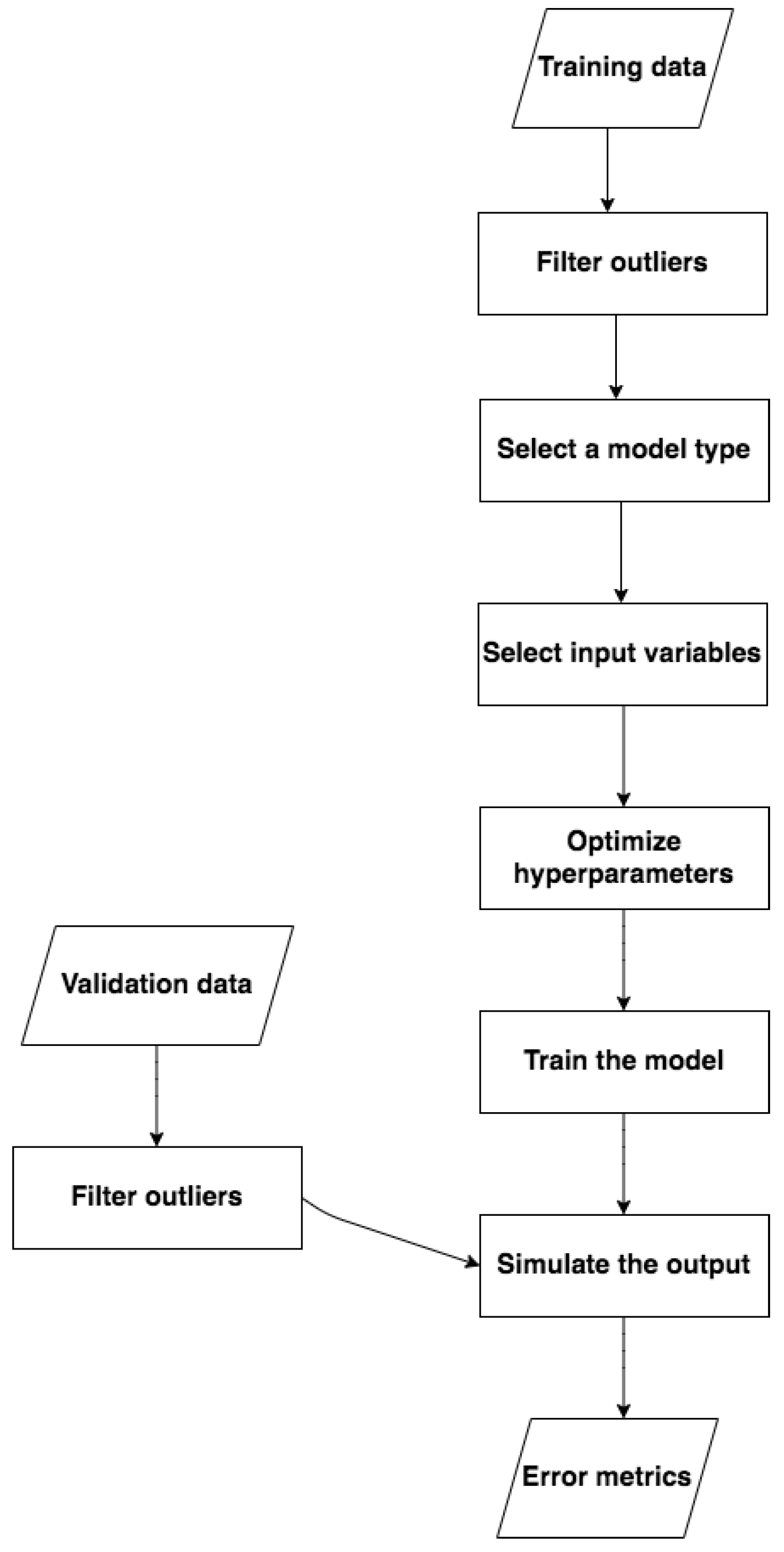
The above steps can be summarized in general through a flow chart (Figure 8) describing the suggested procedure:
- Remove outliers;
- Select a model type;
- Select input variables through Automatic Features Selection algorithms or basing on user’s experience or objectives (as in this case);
- Optimize the set up of the model;
- Train the model;
- Validate the model by predicting the output, given the input variables, on a test data set;
- Analyze the goodness of the regression through appropriate error metrics.
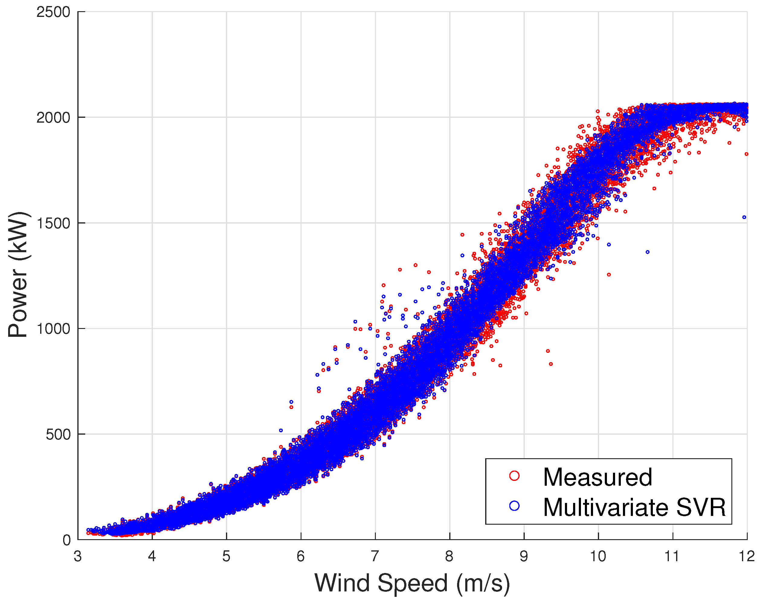
Figure 9 reports the simulated and measured curves for the validation data set. From the Figure, it can be qualitatively appreciated that a multivariate approach allows simulating reliably the dispersion of a real-world power curve. The goodness of the regression can be quantified through the most commonly employed error metrics, such as the MAE and RMSE.
Given the measurements for the validation data set and the model estimates , the residuals are defined in Equation (5):
The MAE is defined in Equation (6):
where N is the number of samples in the validation data set. The is defined in Equation (7):
where is the average residual in the validation data set.
The MAE and RMSE for the example reported in Figure 9 are 20.1 kW and 36.3 kW, respectively. The MAE is of order of 1% of the rated power.
From the discussion in Section 2, it arises that the rotor speed is a very important covariate for wind turbine power monitoring. Actually, in the literature, the concept of rotor equivalent wind speed has been formulated [39,40] for addressing the issue of the effect of the wind shear on wind speed measurements. This idea, as discussed also in Section 1, originates from the fact that nacelle anemometers are affected by several critical points affecting the quality of the measurement [18]. They are placed behind the rotor span and a nacelle transfer function reconstructs the undisturbed flow, but this depends heavily on ambient conditions. The rotor speed instead is regulated only on the grounds of the torque which is exerted on the rotor; therefore, despite that the rotor practically acts as a low-pass filter cutting high-frequency fluctuations and therefore potentially eliminating information, the rotor speed can be considered a reliable probe of on-site conditions.
In this perspective, a more radical interpretation can be conceived. It could be desirable to formulate multivariate models which do not employ nacelle anemometer measurements and to compensate using working parameters. This is challenging because, as discussed in [22], the wind speed explains up to 97% of the variance of the power, but the preliminary results obtained for this study are promising. The performed test consists of considering the same case as above and the same regression type, but the input variables are only the rotor speed, the generator speed and the blade pitch, without the wind speed. The obtained MAE is 21.7 kW and the RMSE is 40.2 kW (summarized in Table 2). Remarkably, the error metrics increase only in the order of 10% with respect to the regression including the wind speed in the input variables. This development is particularly interesting because, also in light of the discussion related to Figure 2, this kind of model could potentially be more reliable for comparing the performance of wind turbines of the same model which are placed in different sites.
As arises from the review in Section 2, there have been several attempts in the literature at formulating input variables selections for wind turbine multivariate power curve models. Nevertheless, it should be noticed that the SCADA data sets are in general under exploited because they contain several dozens of measurement channels, which could in principle be employed. As observed for example in [19], a modern SCADA data set of a wind turbine contains an order of 150 measurement channels and there is no reason why there has been so little exploration about it. Some interesting considerations have been proposed for example in [31,33] about the use of internal temperatures as covariates for wind turbine power curves, but they are substantially early stages analysis. Up to now, the selection of the working parameters has been typically performed basing on considerations similar to Equation (3). The most selected operation variables are rotor speed, blade pitch and possibly the yaw error.
In the author’s opinion, an interesting aspect regards the fact that it should be noticed that the SCADA control systems record and store average, minimum, maximum and standard deviation of each channel in the sampling time (which typically is ten minutes). All the studies cited in Section 2 except [17] use only the average values as covariates, but the use of minimum, maximum and standard deviation could be helpful for improving the regression. This issue has been addressed recently in [16] for the rotor speed, generator speed and blade pitch curves and it arises that the error metrics diminish of approximately one third if one employs as input for the regression also minimum, maximum and standard deviation of the independent variables. This perspective should be investigated in depth as well for multivariate wind turbine power curve modeling. For the purposes of this study, the same test case as above has been analyzed using the same kind of regression and selecting as input variables average, minimum, maximum, standard deviation of wind speed, rotor speed, generator speed, blade pitch. The achieved error metrics (Table 2) are 12.1 kW of MAE and 22.3 kW of RMSE. It is approximately one third less than the metrics for the regression which employs only the average values. It should be noticed that these error metrics, although obtained in a preliminary study, are lower with respect to all the results reported in Section 2 for models employing only SCADA data, because the MAE is approximately 0.5% of the rated power and the AEP is estimated with a precision in the order of 0.3%: this supports the usefulness of this approach to multivariate wind turbine power curve modeling.
On the grounds of this result, it is straightforward to investigate the quality of the regression which excludes the wind speed from the input variables but employs average, minimum, maximum and standard deviation of rotor speed, generator speed and blade pitch. The achieved MAE is 14.3 kW (0.7% of the rated power) and the RMSE is 25.2 kW (Table 2). Additionally in this case, even if the most important covariate (wind speed) has not been used, the error metrics in units of the rated power are lower with respect to the results reported in Table 1. Finally, the results for the regressions discussed in this Section have been normalized to the rated power, in order to facilitate comparison with other studies, and reported in Table 2.
4. Summary
The present manuscript has been devoted to mainly three objectives:
- Summarize the rationale for SCADA-based power curve analysis in wind energy practice and support the use of multivariate approaches;
- Review and discuss in detail the literature regarding data-driven multivariate wind turbine power curve analysis;
- Given the above points, analyze a test case in order to furnish innovative perspectives on the topic.
The main result from the analysis of the literature is that the state-of-the-art regarding multivariate wind turbine power curve analysis is focused on the use of working parameters (as, for example, blade pitch or rotor speed) as further input variables in addition to the wind speed. Actually, it results that meteorological mast data are often unavailable in real-world practice and, most importantly, these kinds of data do not give a remarkable added value: this likely happens because, as supported for example also in [41], the wind flow in operating wind farms might likely be so complex that adding several high-quality meteorological measurements, but concentrated at one point, is not that useful for power curve analysis.
Given this, the main contribution of this study to the topic is the observation that SCADA data sets typically include an order of approximately 150 measurement channels and there has been little exploration about them in the context of multivariate wind turbine power curve analysis. The test case discussed in Section 3 indicates that a straightforward improvement of multivariate power curve regression can consist of the inclusion of minimum, maximum and standard deviation of the main covariates, in addition to the average values. Another interesting consideration regards the fact that sub-component temperatures can likely be very useful covariates because typically they have high correlation with the output power.
The results of a previous study by the author [17] indicate that Automatic Features Selection algorithms, starting from a large set of possible covariates, select different input variables depending on the technology of the wind turbine and on the model type. Therefore, general recommendations can be formulated for a successful multivariate wind turbine power curve regression:
- Use highly non-linear models, like ANN, SVR, GP.
- Start from the vastest set of covariates which is considered potentially meaningful.
- Possibly employ Automatic Features Selection for individuating the most appropriate input variables.
On one hand, multivariate models with a large set of input variables represent an evident complication with respect to the simple wind speed–power curve. Nevertheless, the pros are several because data-driven models employing working parameters and possibly sub-component temperatures can be used not only for more precise performance monitoring, but also for the interpretation of possible anomalies. This more general objective calls for the development of innovative SCADA data analysis methods [42], which in the author’s opinion represent a very fruitful research direction.
Funding
This research received no external funding.
Acknowledgments
The author thanks the company ENGIE Italia for the technical support and for providing the data sets employed for the study.
Conflicts of Interest
The author declares no conflict of interest.
Abbreviations
The following abbreviations are used in this manuscript:
| ANN | Artificial Neural Network |
| IEC | International Electrotechnical Commission |
| GP | Gaussian Process |
| NMAE | Normalized Mean Absolute Error |
| MAE | Mean Absolute Error |
| MAPE | Mean Absolute Percentage Error |
| NRMSE | Normalize Root Mean Square Error |
| NWP | Numerical Weather Prediction |
| RMSE | Root Mean Square Error |
| SCADA | Supervisory Control And Data Acquisition |
| SVR | Support Vector Regression |
| TI | Turbulence Intensity |
References
- Martin, C.M.S.; Lundquist, J.K.; Clifton, A.; Poulos, G.S.; Schreck, S.J. Atmospheric Turbulence Affects Wind Turbine Nacelle Transfer Functions. Wind Energy Sci. 2017, 2, 295–306. [Google Scholar] [CrossRef] [Green Version]
- Honrubia, A.; Vigueras-Rodríguez, A.; Gómez-Lázaro, E. The Influence of Turbulence and Vertical Wind Profile in Wind Turbine Power Curve. Progress in Turbulence and Wind Energy IV; Springer: Berlin, Germany, 2012; pp. 251–254. [Google Scholar]
- International Electrotechnical Commission (IEC). Power Performance Measurements of Electricity Producing Wind Turbines; Technical Report 61400–12; International Electrotechnical Commission: Geneva, Switzerland, 2005. [Google Scholar]
- Wang, Y.; Hu, Q.; Li, L.; Foley, A.M.; Srinivasan, D. Approaches to Wind Power Curve Modeling: A review and Discussion. Renew. Sustain. Energy Rev. 2019, 116, 109422. [Google Scholar] [CrossRef]
- Ciulla, G.; D’Amico, A.; Di Dio, V.; Brano, V.L. Modelling and Analysis of Real-World Wind Turbine Power Curves: Assessing Deviations from Nominal Curve by Neural Networks. Renew. Energy 2019, 140, 477–492. [Google Scholar] [CrossRef]
- You, M.; Liu, B.; Byon, E.; Huang, S.; Jin, J.J. Direction-Dependent Power Curve Modeling for Multiple Interacting Wind Turbines. IEEE Trans. Power Syst. 2017, 33, 1725–1733. [Google Scholar] [CrossRef]
- Hedevang, E. Wind Turbine Power Curves Incorporating Turbulence Intensity. Wind Energy 2014, 17, 173–195. [Google Scholar] [CrossRef]
- Barber, S.; Nordborg, H. Improving Site-Dependent Power Curve Prediction Accuracy Using Regression Trees. J. Phys. Conf. Ser. IOP Publ. 2020, 1618, 062003. [Google Scholar] [CrossRef]
- Shokrzadeh, S.; Jozani, M.J.; Bibeau, E. Wind Turbine Power Curve Modeling Using Advanced Parametric and Nonparametric Methods. IEEE Trans. Sustain. Energy 2014, 5, 1262–1269. [Google Scholar] [CrossRef]
- Bilgili, M.; Tontu, M.; Sahin, B. Aerodynamic Rotor Performance of a 3300-kW Modern Commercial Large-Scale Wind Turbine Installed in a Wind Farm. J. Energy Resour. Technol. 2021, 143, 031302. [Google Scholar] [CrossRef]
- Ackermann, T. Wind Power in Power Systems; John Wiley & Sons: Chichester, UK, 2005. [Google Scholar]
- Pandit, R.K.; Infield, D. Comparative Analysis of Binning and Gaussian Process based Blade Pitch Angle Curve of a Wind Turbine for the Purpose of Condition Monitoring. J. Phys. Conf. Ser. 2018, 1102, 012037. [Google Scholar] [CrossRef]
- Pandit, R.K.; Infield, D. Comparative Assessments of Binned and Support Vector Regression-based Blade Pitch Curve of a Wind Turbine for the Purpose of Condition Monitoring. Int. J. Energy Environ. Eng. 2019, 10, 181–188. [Google Scholar] [CrossRef] [Green Version]
- Pandit, R.; Infield, D. Gaussian Process Operational Curves for Wind Turbine Condition Monitoring. Energies 2018, 11, 1631. [Google Scholar] [CrossRef] [Green Version]
- Astolfi, D.; Byrne, R.; Castellani, F. Analysis of Wind Turbine Aging through Operation Curves. Energies 2020, 13, 5623. [Google Scholar] [CrossRef]
- Astolfi, D. Wind Turbine Operation Curves Modelling Techniques. Electronics 2021, 10, 269. [Google Scholar] [CrossRef]
- Astolfi, D.; Castellani, F.; Lombardi, A.; Terzi, L. Multivariate SCADA Data Analysis Methods for Real-World Wind Turbine Power Curve Monitoring. Energies 2021, 14, 1105. [Google Scholar] [CrossRef]
- Rabanal, A.; Ulazia, A.; Ibarra-Berastegi, G.; Sáenz, J.; Elosegui, U. MIDAS: A Benchmarking Multi-Criteria Method for the Identification of Defective Anemometers in Wind Farms. Energies 2019, 12, 28. [Google Scholar] [CrossRef] [Green Version]
- Schlechtingen, M.; Santos, I.F.; Achiche, S. Using Data-Mining Approaches for Wind Turbine Power Curve Monitoring: A Comparative Study. IEEE Trans. Sustain. Energy 2013, 4, 671–679. [Google Scholar] [CrossRef]
- Lee, G.; Ding, Y.; Genton, M.G.; Xie, L. Power Curve Estimation with Multivariate Environmental Factors for Inland and Offshore Wind Farms. J. Am. Stat. Assoc. 2015, 110, 56–67. [Google Scholar] [CrossRef] [Green Version]
- Pandit, R.K.; Infield, D.; Carroll, J. Incorporating Air Density into a Gaussian Process Wind Turbine Power Curve Model for Improving Fitting Accuracy. Wind Energy 2019, 22, 302–315. [Google Scholar] [CrossRef] [Green Version]
- Janssens, O.; Noppe, N.; Devriendt, C.; Van de Walle, R.; Van Hoecke, S. Data-driven multivariate power curve modeling of offshore wind turbines. Eng. Appl. Artif. Intell. 2016, 55, 331–338. [Google Scholar] [CrossRef]
- Burton, T.; Jenkins, N.; Sharpe, D.; Bossanyi, E. Wind Energy Handbook; John Wiley & Sons: Chichester, UK, 2011. [Google Scholar]
- Campagnolo, F.; Weber, R.; Schreiber, J.; Bottasso, C.L. Wind tunnel testing of wake steering with dynamic wind direction changes. Wind Energy Sci. 2020, 5, 1273–1295. [Google Scholar] [CrossRef]
- Dai, J.; Yang, X.; Hu, W.; Wen, L.; Tan, Y. Effect investigation of yaw on wind turbine performance based on SCADA data. Energy 2018, 149, 684–696. [Google Scholar] [CrossRef]
- Astolfi, D.; Castellani, F.; Becchetti, M.; Lombardi, A.; Terzi, L. Wind Turbine Systematic Yaw Error: Operation Data Analysis Techniques for Detecting It and Assessing Its Performance Impact. Energies 2020, 13, 2351. [Google Scholar] [CrossRef]
- Pelletier, F.; Masson, C.; Tahan, A. Wind turbine power curve modelling using artificial neural network. Renew. Energy 2016, 89, 207–214. [Google Scholar] [CrossRef]
- Manobel, B.; Sehnke, F.; Lazzús, J.A.; Salfate, I.; Felder, M.; Montecinos, S. Wind turbine power curve modeling based on Gaussian processes and artificial neural networks. Renew. Energy 2018, 125, 1015–1020. [Google Scholar] [CrossRef]
- Pandit, R.K.; Infield, D.; Kolios, A. Gaussian process power curve models incorporating wind turbine operational variables. Energy Rep. 2020, 6, 1658–1669. [Google Scholar] [CrossRef]
- Shetty, R.P.; Sathyabhama, A.; Pai, P.S. Comparison of modeling methods for wind power prediction: A critical study. Front. Energy 2020, 14, 347–358. [Google Scholar] [CrossRef]
- Cascianelli, S.; Astolfi, D.; Costante, G.; Castellani, F.; Fravolini, M.L. Experimental Prediction Intervals for Monitoring Wind Turbines: An Ensemble Approach. In Proceedings of the 2019 International Conference on Control, Automation and Diagnosis (ICCAD), Grenoble, France, 2–4 July 2019; pp. 1–6. [Google Scholar]
- Karamichailidou, D.; Kaloutsa, V.; Alexandridis, A. Wind turbine power curve modeling using radial basis function neural networks and tabu search. Renew. Energy 2021, 163, 2137–2152. [Google Scholar] [CrossRef]
- Astolfi, D.; Castellani, F.; Natili, F. Wind Turbine Multivariate Power Modeling Techniques for Control and Monitoring Purposes. J. Dyn. Syst. Meas. Control 2021, 143, 034501. [Google Scholar] [CrossRef]
- De Caro, F.; Vaccaro, A.; Villacci, D. Adaptive wind generation modeling by fuzzy clustering of experimental data. Electronics 2018, 7, 47. [Google Scholar] [CrossRef] [Green Version]
- Astolfi, D.; Byrne, R.; Castellani, F. Estimation of the Performance Aging of the Vestas V52 Wind Turbine through Comparative Test Case Analysis. Energies 2021, 14, 915. [Google Scholar] [CrossRef]
- Byrne, R.; Astolfi, D.; Castellani, F.; Hewitt, N.J. A Study of Wind Turbine Performance Decline with Age through Operation Data Analysis. Energies 2020, 13, 2086. [Google Scholar] [CrossRef] [Green Version]
- Castellani, F.; Astolfi, D.; Natili, F. SCADA Data Analysis Methods for Diagnosis of Electrical Faults to Wind Turbine Generators. Appl. Sci. 2021, 11, 3307. [Google Scholar] [CrossRef]
- Fushiki, T. Estimation of prediction error by using K-fold cross-validation. Stat. Comput. 2011, 21, 137–146. [Google Scholar] [CrossRef]
- Wagner, R.; Cañadillas, B.; Clifton, A.; Feeney, S.; Nygaard, N.; Poodt, M.; St Martin, C.; Tüxen, E.; Wagenaar, J. Rotor equivalent wind speed for power curve measurement–comparative exercise for IEA Wind Annex 32. J. Phys. Conf. Ser. IOP Publ. 2014, 524, 012108. [Google Scholar] [CrossRef]
- Scheurich, F.; Enevoldsen, P.B.; Paulsen, H.N.; Dickow, K.K.; Fiedel, M.; Loeven, A.; Antoniou, I. Improving the accuracy of wind turbine power curve validation by the rotor equivalent wind speed concept. J. Phys. Conf. Ser. 2016, 753, 10–1088. [Google Scholar] [CrossRef] [Green Version]
- Ding, Y.; Kumar, N.; Prakash, A.; Kio, A.E.; Liu, X.; Liu, L.; Li, Q. A case study of space-time performance comparison of wind turbines on a wind farm. Renew. Energy 2021, 171, 735–746. [Google Scholar] [CrossRef]
- Ding, Y. Data Science for Wind Energy; CRC Press: Boca Raton, FL, USA, 2019. [Google Scholar]
Figure 1.
Example of scattered power curve and IEC power curve.

Figure 2.
Example of power curve for a moderate turbulence and a high turbulence site, Vestas V52 wind turbine.
Figure 2.
Example of power curve for a moderate turbulence and a high turbulence site, Vestas V52 wind turbine.

Figure 3.
Example of scattered wind speed–blade pitch curve.

Figure 4.
Example of scattered wind speed–rotor speed curve.

Figure 5.
Example of scattered power–rotor speed curve.

Figure 6.
Example of scattered power–generator speed curve.

Figure 7.
Example of scattered power–blade pitch curve.

Figure 8.
Flowchart of a multivariate wind turbine power curve regression.

Figure 9.
Example of scattered power curve and simulated power curve through a Support Vector Regression (using average wind speed, rotor speed, generator speed, blade pitch).
Figure 9.
Example of scattered power curve and simulated power curve through a Support Vector Regression (using average wind speed, rotor speed, generator speed, blade pitch).


Table 1.
Summary of model structures, data sources, input variables selection (in addition to the wind speed) and results for the literature about multivariate wind turbine power curve.
Table 1.
Summary of model structures, data sources, input variables selection (in addition to the wind speed) and results for the literature about multivariate wind turbine power curve.
| Ref. | Model | Data | Input Variables | Error |
|---|---|---|---|---|
| [19] | Cluster center fuzzy logic ANN k-nearest neighbors Adaptive neuro-fuzzy interference model | SCADA | Wind direction Ambient temperature | NMAE: 1.9% |
| [20] 1 | Additive kernel density | SCADA + Met mast | Wind direction Air density Humidity Turbulence intensity Wind Shear 1 Wind Shear 2 | NRMSE: 34.9% |
| [20] 2 | Additive kernel density | SCADA + Met mast | Wind direction Air density Turbulence intensity Wind Shear 1 | NRMSE: 15.9% |
| [22] | Random forest Extremely randomized trees Stochastic gradient regression trees k-nearest neighbors Binning method 5-parameters logistic | SCADA | Wind direction Yaw error Blade pitch Rotor speed | MAE: 59 kW |
| [27] | ANN | SCADA + Met mast | Wind direction Air density Turbulence intensity Yaw error | MAE: 15.3 kW |
| [28] | Gaussian process + ANN | SCADA | Wind direction | NMAE: 1.34% |
| [29] 1 | Gaussian process | SCADA | Air density Blade pitch | NMAE: 1.64% |
| [29] 2 | Gaussian process | SCADA | Air density Rotor speed | NMAE: 1.13% |
| [29] 3 | Gaussian process | SCADA | Air density Blade pitch Rotor speed | NMAE: 1.07% |
| [30] | Least squares Cubic spline ANN Response surface | SCADA | Air density Blade pitch Rotor speed | NRMSE: 0.96% |
| [5] | ANN | SCADA + Met mast | 12 meteo variables | NRMSE: 2.41% |
| [31] | Polynomial LARS | SCADA | Wind direction Turbulence intensity Ambient temperature Rotor speed Blade pitch Yaw error 18 internal temperatures | NRMSE: 1.71% |
| [32] | Radial basis ANN + Tabu search | SCADA | Wind direction Ambient temperature Blade pitch | NMAE: 1.28% |
| [33] | Principal component linear Support vector Feedforward ANN | SCADA | Ambient temperature Blade pitch Rotor speed 1 internal temperature | NMAE: 1.27% |
| [17] | Support vector | SCADA | Blade pitch Rotor speed Generator speed | NMAE: 0.87%–1.39% |
Table 2.
Input variables selection and error metrics for the discussion test case.
| Input Variables | NMAE (%) | NRMSE (%) |
|---|---|---|
| Wind speed (Avg.) Blade pitch (Avg.) Rotor speed (Avg.) Generator speed (Avg.) | 0.98 | 1.77 |
| Blade pitch (Average) Rotor speed (Average) Generator speed (Average) | 1.05 | 1.96 |
| Wind speed (Avg., Min., Max., Std. Dev.) Blade pitch (Avg., Min., Max., Std. Dev.) Rotor speed (Avg., Min., Max., Std. Dev.) Generator speed (Avg., Min., Max., Std. Dev.) | 0.59 | 1.08 |
| Blade pitch (Avg., Min., Max., Std. Dev.) Rotor speed (Avg., Min., Max., Std. Dev.) Generator speed (Avg., Min., Max., Std. Dev.) | 0.69 | 1.22 |
Publisher’s Note: MDPI stays neutral with regard to jurisdictional claims in published maps and institutional affiliations. |
© 2021 by the author. Licensee MDPI, Basel, Switzerland. This article is an open access article distributed under the terms and conditions of the Creative Commons Attribution (CC BY) license (https://creativecommons.org/licenses/by/4.0/).
Share and Cite
MDPI and ACS Style
Astolfi, D. Perspectives on SCADA Data Analysis Methods for Multivariate Wind Turbine Power Curve Modeling. Machines 2021, 9, 100. https://0-doi-org.brum.beds.ac.uk/10.3390/machines9050100
AMA Style
Astolfi D. Perspectives on SCADA Data Analysis Methods for Multivariate Wind Turbine Power Curve Modeling. Machines. 2021; 9(5):100. https://0-doi-org.brum.beds.ac.uk/10.3390/machines9050100
Chicago/Turabian StyleAstolfi, Davide. 2021. "Perspectives on SCADA Data Analysis Methods for Multivariate Wind Turbine Power Curve Modeling" Machines 9, no. 5: 100. https://0-doi-org.brum.beds.ac.uk/10.3390/machines9050100
Note that from the first issue of 2016, this journal uses article numbers instead of page numbers. See further details here.