
Fault Diagnosis of Rolling Bearing Based on Shift Invariant Sparse Feature and Optimized Support Vector Machine


1
College of Information Science and Technology, Donghua University, Shanghai 201620, China
2
School of Mechatronic Engineering and Automation, Shanghai University, Shanghai 200444, China
*
Author to whom correspondence should be addressed.
Machines 2021, 9(5), 98; https://0-doi-org.brum.beds.ac.uk/10.3390/machines9050098
Submission received: 12 April 2021
/
Revised: 30 April 2021
/
Accepted: 8 May 2021
/
Published: 12 May 2021
(This article belongs to the Section Machines Testing and Maintenance)
Abstract
:The vibration signal of rotating machinery fault is a periodic impact signal and the fault characteristics appear periodically. The shift invariant K-SVD algorithm can solve this problem effectively and is thus suitable for fault feature extraction of rotating machinery. With the over-complete dictionary learned by the training samples, including thedifferent classes, shift invariant sparse feature for the training as well as test samples can be formed through sparse codes and employed as the input of classifier. A support vector machine (SVM) with optimized parameters has been extensively used in intelligent diagnosis of machinery fault. Hence, in this study, a novel fault diagnosis method of rolling bearings using shift invariant sparse feature and optimized SVM is proposed. Firstly, dictionary learning by shift invariant K-SVD algorithm is conducted. Then, shift invariant sparse feature is constructed with the learned over-complete dictionary. Finally, optimized SVM is employed for classification of the shift invariant sparse feature corresponding to different classes, hence, bearing fault diagnosis is achieved. With regard to the optimized SVM, three methods including grid search, generic algorithm (GA), and particle swarm optimization (PSO) are respectively carried out. The experiment results show that the shift invariant sparse feature using shift invariant K-SVD can effectively distinguish the bearing vibration signals corresponding to different running states. Moreover, optimized SVM can significantly improve the diagnosis precision.
1. Introduction
Sparse representation has been widely employed in image, video, and speech signal processing [1,2,3]. In recent years, a growing number of researchers utilize sparse representation to machinery fault diagnosis and performance degradation assessment [4]. Yu et al. proposed a novel classification method based on group sparse representation for bearing and gear fault diagnosis [5]. Peng et al. applied sparse representation to extract bearing fault features [6]. Fan et al. put forward a transient feature extraction method using sparse representation in wavelet basis [7].
For sparse representation, we can construct an over-complete dictionary through predefined dictionary, which needs prior knowledge of the signals, and is therefore not feasible in an engineering practice. The dictionary can also be formed by randomly choosing some samples from the training samples if the number of training samples is large enough. However, if the dataset is very large, this method does not work well, therefore we need more effective dictionary learning algorithms, e.g., K-means singular value decomposition (K-SVD) [8], method of optimal directions (MOD) [9], etc. K-SVD algorithm was first proposed for processing images and has been extensively applied to image processing [10,11,12]. In machinery fault diagnosis, K-SVD has also been employed. Zhu put forward a cutting force denoising method for micro-milling condition monitoring with modified K-SVD [13]. Zeng et al. implemented group-based K-SVD denoising algorithm for bearing fault diagnosis [14].
If the long signal has the same internal structure, namely a pattern that recurs periodically, namely these internal structures will be translated to different positions in the long signal, which is called shift invariant. In this case, the same dictionary atom, namely the base function, can be used to express the internal pattern of the signal, regardless of its moving position, while the shift invariant dictionary learning algorithm can solve this problem. Some shift invariant dictionary learning algorithms have been put forward, e.g., shift invariant sparse coding [15], convolutional sparse representation [16], shift invariant K-SVD [17], etc. In the fault vibration signal of rotating machinery, there exists periodic recurrence impulses, hence, shift invariant dictionary learning algorithm is particularly suitable to diagnose the fault of rotating machinery. Recently, these algorithms have been used for mechanical fault diagnosis. Liu et al. used shift-invariant sparse coding for feature extraction and achieved fault diagnosis of rolling bearings [18]. Feng et al. utilized shift invariant K-SVD to acquire vibration patterns hidden in planetary gearbox signals with strong background noise [19]. Tang et al. implemented shift invariant sparse coding to realize bearing and gear fault detection [20]. Chen et al. combined shift invariant K-SVD with the Wigner-Ville distribution and applied it to fault diagnosis of wind turbine bearings [21]. Ding put forward a fault diagnosis method based on convolution sparse coding and applied it to wheelset bearing in high-speed train [22]. Li et al. put forward a shift-invariant manifold learning method to enhance the transient characteristics of bearing fault [23]. Ding et al. put forward a sparse feature extraction method using periodic convolution sparse representation and applied it to machinery fault detection [24]. He et al. combined convolutional sparse representation with bandwidth optimization and proposed a fault detection method for wheelset bearing [25]. Zhou et al. put forward a new method for the diagnosis of bearing fault using shift-invariant dictionary learning and hidden Markov model [26]. In this paper, shift invariant K-SVD algorithm is conducted to generate sparse feature of the vibration signals of rolling bearing.
After feature extraction, the intelligent machinery fault diagnosis is the problem of classification, which belongs to the problem of pattern recognition. Thus, the pattern recognition methods can be used, e.g., support vector machine (SVM) [27,28,29,30,31], artificial neural network (ANN) [32], deep learning [33], etc. Compared with neural network, SVM [34] utilizes structural risk minimization, and can thus avoid over-fitting, local minimization, and low convergence speed. Besides, SVM is more effective for training samples with a small number and high dimension. When the data cannot be linearly discriminated, a kernel function which can translate the data to high dimensional feature space is always utilized in SVM, where the radial basis function (RBF) kernel is the most broadly employed. The discrimination ability of SVM is greatly affected by the parameters including kernel function parameter and penalization factor, hence it is very essential to conduct the optimization of the parameters by means of intelligent evolutionary algorithms, e.g., particle swarm optimization (PSO) [35] and generic algorithm (GA) [36,37]. For machinery fault diagnosis, SVM with optimized parameters has been widely used. Lu et al. applied an adaptive feature extraction method and optimized SVM based on PSO to drivetrain gearbox fault diagnosis [29]. Wang et al. utilized SVM based on GA to realize bearing fault diagnosis [30]. Three methods including grid search, GA, and PSO are respectively conducted to optimize SVM in this paper.
In this study, a novel method using shift invariant sparse feature and optimized SVM is put forward to realize bearing fault diagnosis. First of all, shift invariant K-SVD is adopted to learn an over-complete dictionary, whose training samples come from the vibration signals of rolling bearings at different running states. After that, the shift invariant sparse feature is constructed through sparse codes solved by the learned dictionary, which can be used as the input of SVM. In the end, optimized SVM using three different methods is implemented to distinguish different running states of rolling bearings including normal state, the fault of inner race, outer race and rolling element, hence intelligent fault diagnosis of rolling bearings can be achieved.
The remaining part of the paper includes: Section 2 introduces feature extraction method with shift invariant K-SVD. In Section 3, the pattern recognition method using optimized SVM is demonstrated. Then, the proposed bearing fault diagnosis model is presented in Section 4. Subsequently in Section 5, the experiment of rolling bearing fault is conducted to validate the effectiveness of the proposed method. At last, in Section 6, the conclusion is acquired.
2. Feature Extraction Using Shift Invariant K-SVD Algorithm
With regard to periodic impact signals, the same fault mode appears repeatedly at different times, which shows shift invariant characteristics. However, when using the K-SVD dictionary learning method, the learned dictionary will demonstrate that multiple different basis functions belong to the same fault feature mode, which just correspond to the different impact positions, that is, the K-SVD algorithm does not consider the shift invariant characteristics in the periodic impact signals, while the shift invariant K-SVD algorithm (SI-KSVD) [16] can effectively solve this problem, in which each fault mode, namely basis function, can appear at any moment and a translation of the same basis function is conducted to represent the periodically recurring signal characteristics. Although the fault characteristics may be submerged in strong noise and interference, the characteristic of periodic recurrence makes the shift-invariant K-SVD algorithm easier to converge to these recurring characteristic patterns. Therefore, a shift-invariant K-SVD algorithm is very suitable to extract the feature of periodic impact signals and thus a sparse feature based on shift invariant K-SVD algorithm can be formed.
In summary, for the feature extraction method using shift invariant K-SVD, there are two stages: dictionary learning and sparse coefficients solving. Firstly, dictionary learning using shift-invariant K-SVD is carried out to obtain a redundant dictionary. Afterwards, sparse codes can be solved, and the discriminative sparse feature is constructed based on the sparse codes.
2.1. Shift Invariant K-SVD Algorithm
For a long signal , assuming that there are a total of K basis functions , each basis function corresponds to a characteristic pattern and the over-complete dictionary D is constructed by translating a series of basis functions in the time domain. The goal of shift invariant K-SVD is to obtain several basis functions through dictionary learning based on a long signal x, thereby forming a total over-complete dictionary D, whose objective function is [17]:
where is the shift operator that translates the basis function to time τ and extends it to obtain a dictionary atom with the same length as the original long signal, where the basis function in this atom starts at time τ and all the rest is set to 0. For each basis function of length q, it can be translated up to time p − q + 1 and thus forming a total of p − q + 1 dictionary atoms and the total over-complete dictionary D contains K × (p − q + 1) dictionary atoms. is the sparse coefficient with respect to the dictionary atom after basis function is translated to time τ and extended. s is the sparse coefficient vector of the long signal x and T is the sparsity prior.
Similar to the two-step iterative process of the K-SVD dictionary learning algorithm, the shift invariant K-SVD algorithm is also a two-step iterative algorithm, which includes the sparse coefficient solving stage and the dictionary updating stage. During the sparse coefficient solving stage, each basis function is fixed. Due to excessive atoms of the over-complete dictionary, the calculation is very time-consuming. Using the fast matching pursuit algorithm [38] can greatly improve the computing efficiency. During the dictionary update stage, each basis function is updated in sequence. When the basis function is updated, other basis functions remain fixed and the sparse coefficients of the dictionary atoms corresponding to the basis function are also updated.
In the dictionary update stage, for a given basis function or feature pattern , let the activation part in the corresponding coefficients be obtained in the first step of sparse decomposition stage, namely the set of non-zero elements be , defining the signal with no contribution from other basis functions , as shown below:
where r is the residual signal. From Equation (1), the optimal basis function can be updated by the following equation:
The above equation can be expressed:
where is the operator corresponding to , which can extract a segment with the same length q as the basis function from the long signal and the segment starts at time τ.
Using only the activation information corresponding to the basis function in the first sparse decomposition stage, i.e., the set of non-zero coefficients , the sparse coefficient and the new basis functions can be simultaneously updated. By Equation (4), the matrix formed by the basis function and the segment corresponding to can be obtained and then the singular value decomposition can be performed on it. After the singular value decomposition, the largest singular value is retained, which means that the first principal component can be selected to obtain the best basis function and corresponding sparse coefficients:
The flow of shift invariant K-SVD algorithm is as follows:
(1) Given the long signal x and the length q and number K of basis functions. The initial basis functions are formed by randomly truncating segments with length q from the long signal x and then normalizing the segments. Set the number of iterations t = 1 and tolerance error ;
(2) Solving the sparse coefficient stage. The fast-matching pursuit algorithm is conducted to obtain the sparse coefficient s corresponding to the long signal;
(3) Basis function update stage. Each basis function is updated in turn and assuming that when updated to the k-th basis function , defining the set of sparse coefficients activated by the basis function , thus the basis function and the corresponding sparse coefficient can be updated through Equations (5) and (6);
(4) Let and judge whether the iteration is terminated. If the ratio of the reconstruction error of the two adjacent iterations is less than , the iteration is terminated, otherwise steps (2)–(4) are repeated.
If there are multiple long signals forming a training set X, shift invariant K-SVD can still be utilized to learn the basis functions. Firstly, shift invariant K-SVD algorithm is employed for the first long signal , where the initial basis functions is constructed by randomly truncating segments from the long signals and then be normalized. Through this learning, sparse coefficients and corresponding basis functions can be obtained. The basis functions obtained through the shift invariant dictionary learning is more capable of sparsely representing the signal sample than the previous initial basis functions, which means that is closer to the nature of the signal . Then, is used as the initial basis functions and shift invariant K-SVD algorithm is applied to the second long signal , thus sparse coefficients and corresponding basis functions can be obtained. After that, is used as the initial basis functions and shift invariant K-SVD is applied to the third long signal .The above iterative process continues until the last long signal and sparse coefficients and corresponding basis functions are obtained. If the algorithm needs to continue, the basis functions is used as the initial basis functions and shift invariant K-SVD algorithm is applied to the first long signal and then the above iterative process is repeated in the order of the long signal. Whether the algorithm stops or not generally depends on whether the basis functions D has stabilized, which means that the relative error of two adjacent iterations of the basis functions D is less than the tolerance error. Finally, the basis functions D are learned through the algorithm.
2.2. Shift Invariant Sparse Feature
After the shift invariant dictionary learning, K basis functions is obtained. Each basis function is translated in the time domain and extended to the length of the original long signal and then the sub-dictionary corresponding to the basis function can be acquired, which contains p-q+1 dictionary atoms. If there are L classes of signals and each class contains multiple training samples that are long signals, the shift invariant K-SVD algorithm is conducted for each class of samples and the K basis functions are employed for the training samples of each class and thus LK sub-dictionaries can be obtained. Then, a whole redundant dictionary with LK sub-dictionaries can be formed by concatenating the sub-dictionaries. For each signal sample, matching pursuit algorithm is applied based on the over-complete dictionary D to solve the sparse coefficient where corresponds to each sub-dictionary . Afterwards, the l1 norm, l2 norm or maximum absolute value of the sparse coefficient vector corresponding to the sub-dictionary with p − q + 1 dictionary atoms is computed and thus LK-dimensional sparse feature can be obtained for each signal. Moreover, M(M ≥ 2) maximum absolute values of the sparse coefficient vector are also computed, which is denoted as M-Max and thus LKM-dimensional sparse feature can be obtained for each signal. The LK-dimensional or LKM-dimensional sparse feature is named shift invariant sparse feature.
From the perspective of sparse representation, the sub-dictionary with regard to the class of the test sample is more adaptive to the test sample, i.e., the sub-dictionary with regard to the class of the test sample is more likely to be activated to approximate the test sample. Assuming that the class label of test sample yj is , the sub-dictionaries corresponding to the class j are more likely to be activated, i.e., solving the sparse coefficient using the whole over-complete dictionary D and then the non-zero terms in the sparse coefficients corresponding to the sub-dictionaries Di are most likely to appear in , thus the l1 norm, l2 norm or M(M ≥ 1) maximum absolute values of the sparse coefficient vector corresponding to the sub-dictionaries Di are larger than the other sub-dictionaries. Therefore, the shift invariant sparse feature corresponding to different classes is distinguishable and can be employed as the input of classifier.
3. Classification with Optimized SVM
In this study, LIBSVM [39] is applied to the classification task including multiple classes using one-against-one method. RBF kernel is suitable to conduct non-linear classification, where g denotes the width of RBF kernel. Moreover, penalization factor c also has a large impact on SVM performance. Consequently, the parameters (c, g) should be jointly optimized in order to get best SVM. In the following subsections, three different methods including grid search, GA, and PSO are respectively carried out to optimize SVM.
The whole process of optimized SVM is as follows: firstly, linear normalization to [0, 1] is conducted on both the training set and test set; then, based on the training set, cross validation using the different parameters (c, g) is carried out and the best parameters that own the highest cross validation accuracy can be achieved, which is regarded as the best SVM model that corresponds to the training set; at last, the test set is predicted with the best SVM model.
3.1. Grid Search
The parameters (c, g) are given with an interval in grid form and all of the parameters are calculated to search the highest cross validation accuracy.
3.2. Genetic Algorithm
Genetic algorithm (GA) imitates the genetic and evolutionary process of organisms in nature [36], which operates on the coding of the decision variables and takes the objective function as search information while using the information of all points. Hence, GA owns excellent global search ability. The shortcomings of GA are that the local search ability is weak and the result is easily affected by the parameters.
GA consists of the following steps: population initialization, individual evaluation, selection operation, cross operation, mutation operation, and the decision of stopping criterion. In this study, the fitness value of GA is cross validation accuracy of SVM using the training set. With regard to the selection operation, it is to select relatively good individuals from the current population and copy them to the next population. Firstly, the total fitness of all individuals in the population is computed, then the relative fitness of each individual is computed as the individual selection probability, and finally the roulette method is employed to select new individuals. For the cross operation, the crossover operator is applied to the population, and two chromosomes are randomly selected for crossover. Whether to perform the crossover operation or not is determined by the crossover probability. The crossover position is randomly selected and the crossover position of the two chromosomes is the same. With respect to the mutation operation, the mutation operator is applied to the population, and a chromosome is randomly selected for mutation. Whether to perform the mutation operation or not is determined by the mutation probability. The position of the mutation is randomly selected, i.e., which gene is selected for mutation. After the mutation is completed the feasibility of the chromosome is tested.
3.3. Particle Swarm Optimization
PSO is also an evolutionary algorithm [35]. Compared with genetic algorithm, there are no crossover and mutation operations in PSO and the particles are only updated through internal velocity and thus PSO is easier to realize. However, when dealing with a complex problem with a high dimension, PSO always suffers premature convergence and the convergence performance is poor and thus the optimal solution cannot be guaranteed.
Suppose there are N particles in the particle swarm and the ith particle is , (where K represents the parameter numbers that should be optimized, in this study K = 2), whose velocity is expressed by . The fitness value of the ith particle is the cross-validation accuracy of SVM based on pi. In the iteration process, the best value of the ith particle that indicates the local best is represented by pbesti, while the best particle that indicates the global best is represented by gbest. Firstly, the initialization of the particles is implemented by a random number in the specified range. For the kth iteration, the ith particle and its velocity are renewed as follows [35]:
where wv and wp are elastic coefficients for velocity update and particle update, respectively. c1 and c2 are acceleration coefficients, which represents the local and global search ability, respectively. r1 and r2 are random numbers uniformly distributed in [0, 1].
Each iteration indicates one generation, and the termination of iterations is determined by the maximum generations. When the iterations end, the global best value is obtained which signifies the best cross validation accuracy.
4. Bearing Fault Diagnosis Method Using Shift Invariant Sparse Feature and Optimized SVM
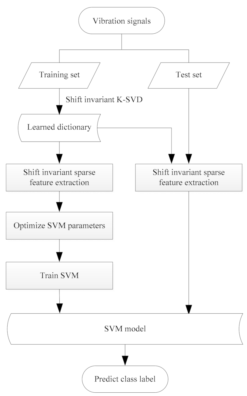
In this paper, a fault diagnosis method for rolling bearing using shift invariant sparse feature and optimized SVM is proposed. There are a total of five stages in the proposed method: dictionary learning with shift invariant K-SVD, sparse feature extraction, optimization of SVM, best SVM training and fault diagnosis. Figure 1 describes the whole process of the proposed method, and the description with regard to each stage is introduced in detail as follows:
(1) Dictionary learning with shift invariant K-SVD. Using the training set, an over-complete dictionary is obtained with shift invariant K-SVD.
(2) Sparse feature extraction. Using the learned over-complete dictionary, sparse feature of all samples can be constructed as shown in Section 2.2, which can be employed as the input of SVM.
(3) Optimization of SVM. Three methods including grid search, GA, and PSO are respectively implemented to get the best (c, g), which has the best cross validation accuracy.
(4) SVM model training. Using the training set, the best SVM model can be learned with the best c and g.
(5) Fault diagnosis. For the test set, the category label of each test sample is predicted through the learned SVM model, therefore fault diagnosis of rolling bearings is achieved.
5. Experiment and Analysis
5.1. Description of the Experiment
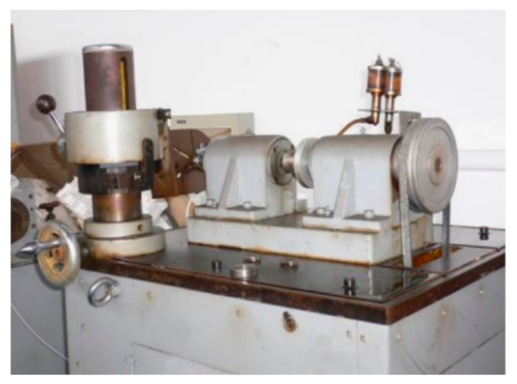
The proposed scheme based on shift invariant sparse feature and optimized SVM is verified by the experiment of rolling bearings fault through artificial processing. Figure 2 shows the test rig [26]. An AC motor drives the shaft through coupling and the shaft is supported by rolling bearings (GB203) at 720 rpm. The vibration signals are acquired by data acquisition system (NI PXI-1042), where the acceleration sensor (Kistler 8791A250) is located on the bracket that is fixed on the rolling bearing and the sampling rate is 25.6 kHz. The electro-discharge machining is carried out on the surface of the outer race, inner race, and rolling element of the rolling bearings, and three different classes of fault containing the fault of outer race (ORF), inner race (IRF) and rolling element (REF) are obtained, respectively. Consequently, including the normal state there are a total of four states.
With respect to the data set, there are a total of 120 samples containing four running states, with 30 samples in each state and each sample containing 20,480 points. Figure 3 describes the vibration signals of the rolling bearings corresponding to the four states. With regard to each sample, truncation is conducted to acquire 10 time series with 2048 points, so 1200 samples in four states can be obtained and each state has 300 samples.
The training set is formed by randomly selecting 150 samples from the 300 samples corresponding to different states, while the test set is constructed by the remaining samples. Hence, the training and test set both containing 600 samples are respectively generated.
5.2. Feature Extraction with Shift Invariant Sparse Feature
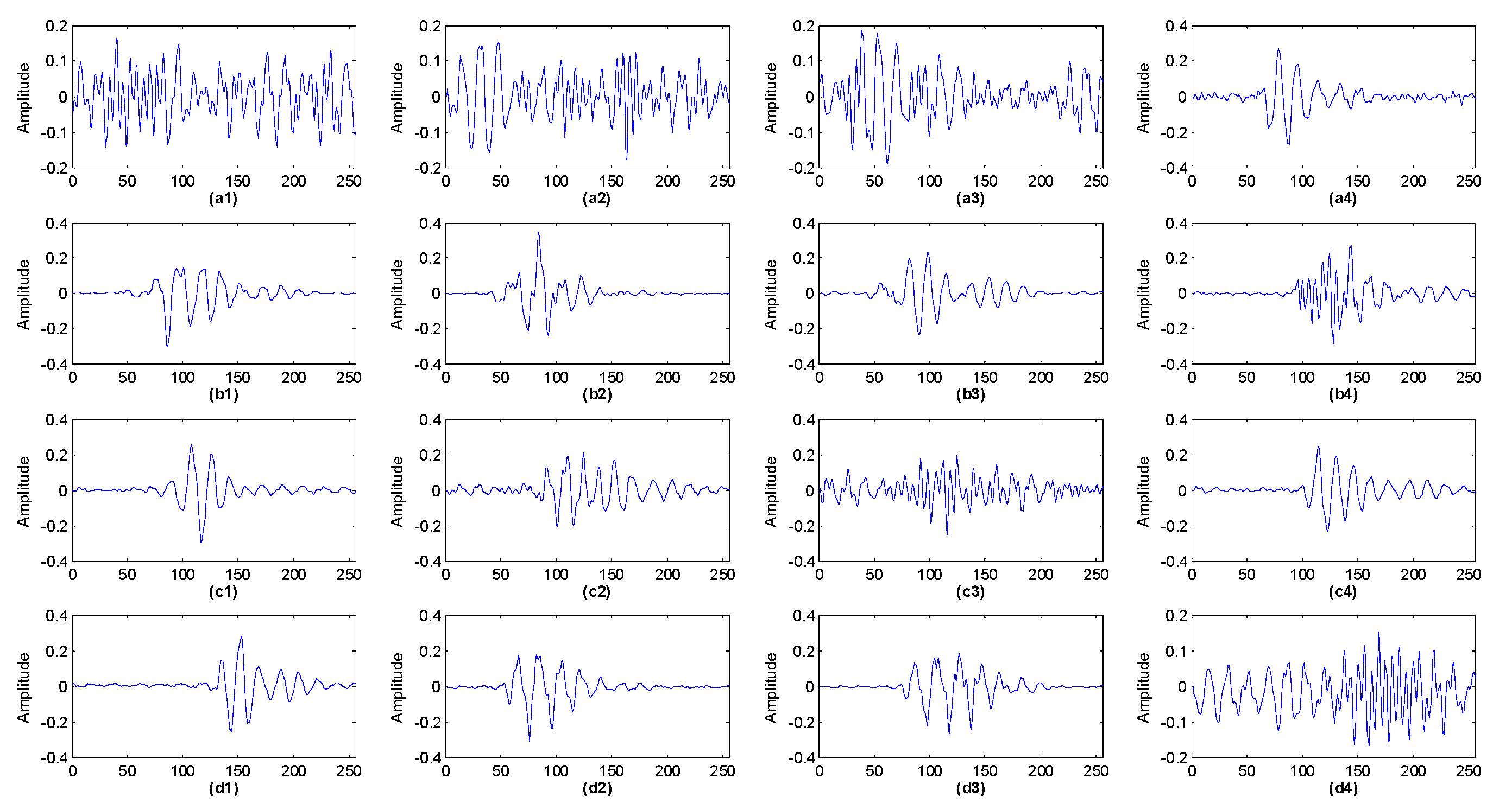
Firstly, based on each class of training samples shift invariant K-SVD algorithm for multiple training samples is carried out to learn the dictionary corresponding to each class. The basis function length is 256 points and the basis function number is 4. When using matching pursuit algorithm for sparse decomposition, the sparsity prior T should be set. Theoretically, the sparsity prior T should be given as the quotient of the original signal length divided by the length of the basis function, but in order to allow correction of the sparse decomposition error, the sparsity can be set to 1.2 times the quotient [19], namely 1.2 × 2048/256 ≈ 10. In addition, the basis function number is generally set to greater than 2. If the basis function number is too large, the calculation amount is greatly increased and most basis functions will converge to noise. Conversely, in case there are too few basis functions, the fault feature components are hard to extract. In this paper, 4 basis functions are selected and the influence of different numbers of basis functions on the classification results is discussed in the next section.
The learned four basis functions corresponding to each class is demonstrated in Figure 4. From the figure, it can be found that the basis functions belonging to different classes are significantly different.
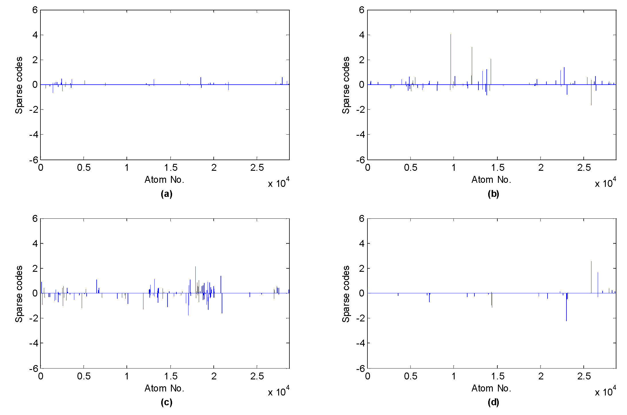
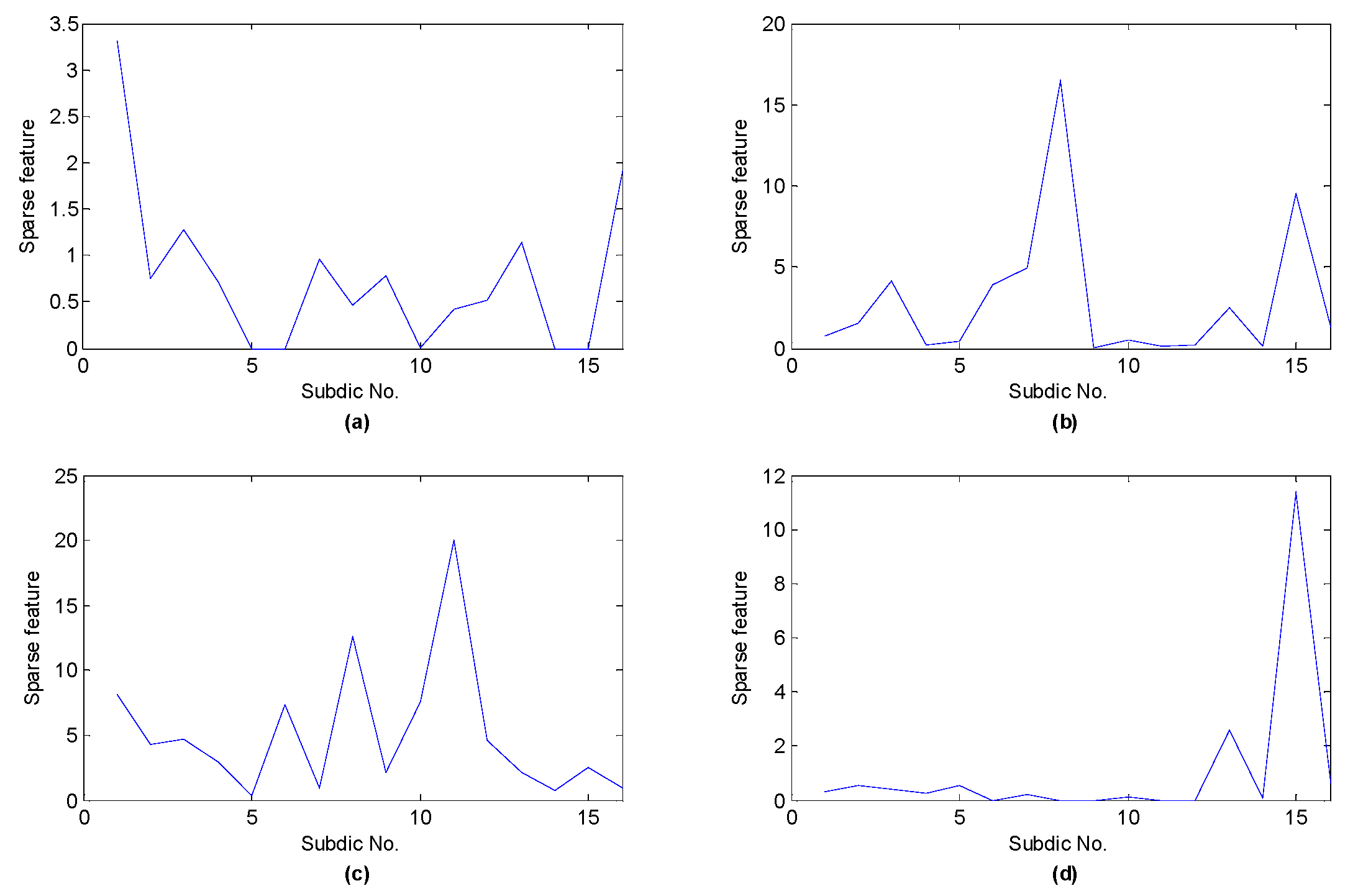
After basis functions with regard to each class have been learned, the sub-dictionaries for each class can be formed, and thus the over-complete dictionary can be constructed by concatenating the sub-dictionaries. Using the over-complete dictionary, the sparse coefficients of all samples are calculated with the sparsity prior 10 and the sparse coefficients of four test samples with respect to four classes are demonstrated in Figure 5. As shown in the figure, each sample is more likely to be activated by the atoms corresponding to the category of the sample. Then, the shift invariant sparse feature can be computed based on the sparse codes and l1 norm, l2 norm or M-Max. Hence, 16-dimensional (l1 norm, l2 norm and Max), 32-dimensional (M = 2), or 48-dimensional (M = 3) feature vector is respectively acquired with regard to each sample.
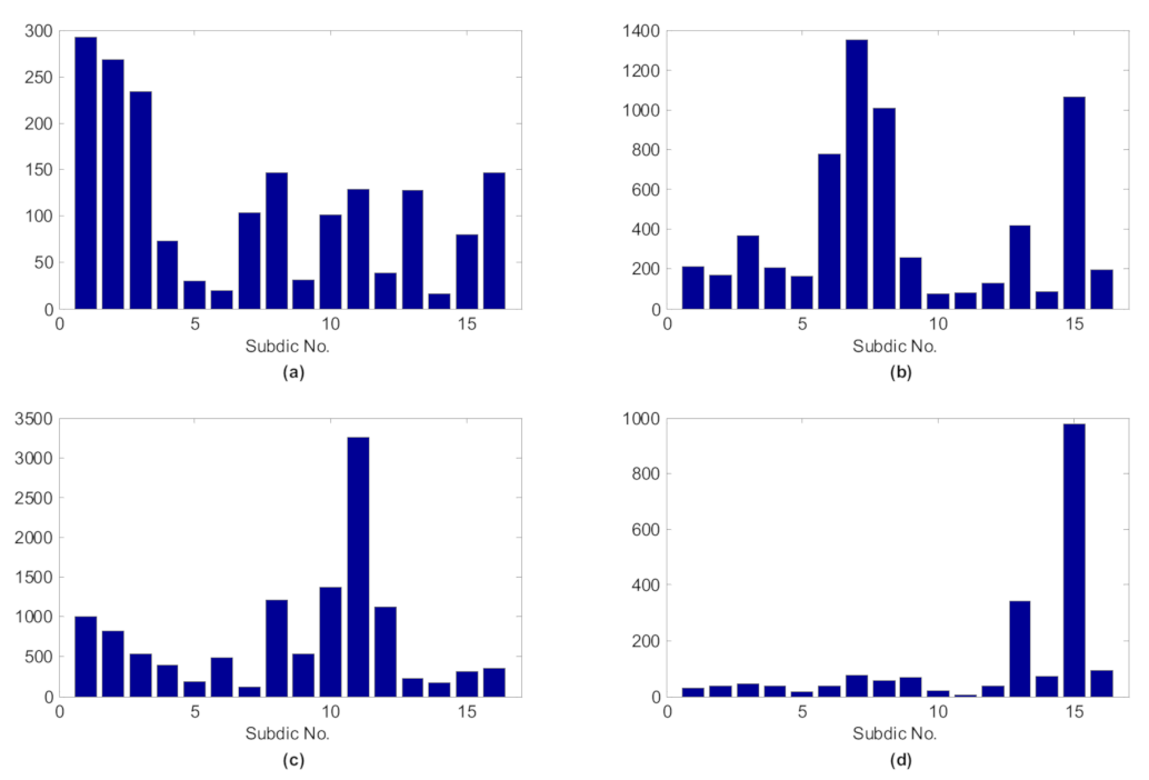
Through the shift invariant K-SVD algorithm, matching pursuit algorithm and l1 norm, the shift invariant sparse feature can be obtained. The test sample randomly selected for four different states and the sum of shift invariant sparse feature of test samples from the same state are demonstrated in Figure 6 and Figure 7, respectively, where the sub-dictionary no. 1~4, 5~8, 9~12, 13~16 denotes normal, the fault of inner race, rolling element and outer race, respectively.
From the above two figures, we can find that for the test samples, the sub-dictionaries corresponding to the class of the samples are more likely to be activated, whose values are significantly larger than other sub-dictionaries, which reveals that shift invariant K-SVD can enable the signals of the same class to produce similar sparse feature, hence the shift invariant sparse feature is discriminative and can be employed as the input feature vector of the classifier.
5.3. Fault Diagnosis Using Shift Invariant Sparse Feature
After the feature of the training set and test set was extracted, SVM was utilized for classification. Firstly, standard SVM, which means that (c, g) are not optimized but specified instead, was employed. Then, the influence of the parameter sets of shift invariant sparse feature was analyzed. In the end, the optimization of SVM was carried out.
5.3.1. Diagnosis Result with Standard SVM
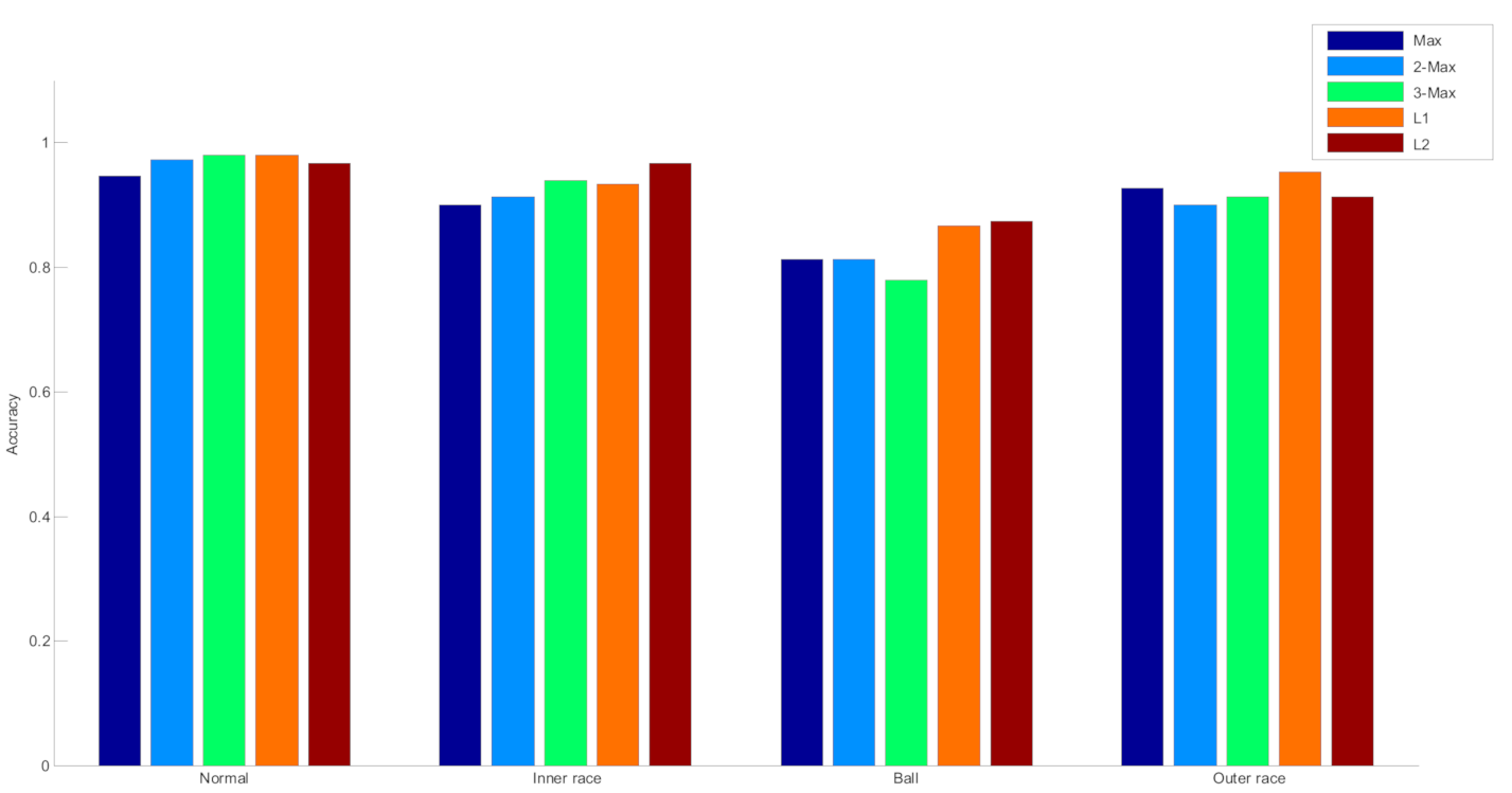
With regard to standard SVM, (c, g) are both set to 1. Based on the same learned over-complete dictionary, different methods for generating sparse feature, there are a total of five feature extraction methods using different sparse feature, including maximum absolute values, 2 maximum absolute values, 3 maximum absolute values, l1 norm and l2 norm, which are denoted as Max, 2-Max, 3-Max, L1, and L2, respectively, whose classification results are demonstrated in Table 1. Figure 8 respectively describes the detailed classification results corresponding to four classes.
Table 1 indicates that the different methods to construct sparse features have great impact on diagnosis result, in which the sparse feature using L1 (l1 norm) achieves the highest accuracy and thus l1 norm is utilized in the subsequent classification task using optimized SVM. The accuracy of the feature extraction method based on Max (Maximum absolute values) is the lowest, which is due to that the Max method ignores a lot of important sparse feature information in the sparse codes. However, with the increase of M, the accuracy is improved. Figure 8 shows that on the whole, the rolling element fault acquired the worst result, which signifies that rolling element fault is very complicated and harder to recognize. For normal and outer race fault, the method based on L1 (l1 norm) outperforms all the other methods.
5.3.2. Influence of Parameter Set of Shift Invariant Sparse Feature
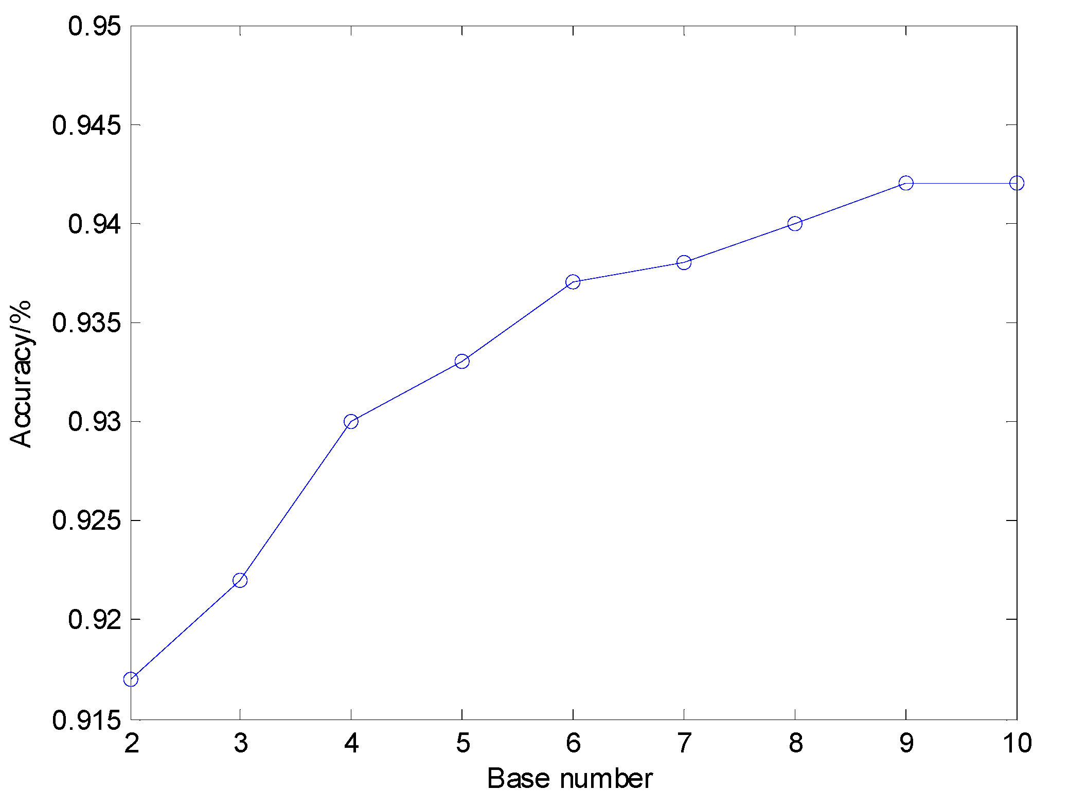
With the feature extraction method based on L1 (l1 norm) and standard SVM, which means (c, g) are both set to 1, the influence of the parameter set of shift invariant sparse feature was discussed. In shift invariant K-SVD algorithm, the number of base functions K for each class has a great influence on the whole fault diagnosis method so different K varying from was respectively conducted.
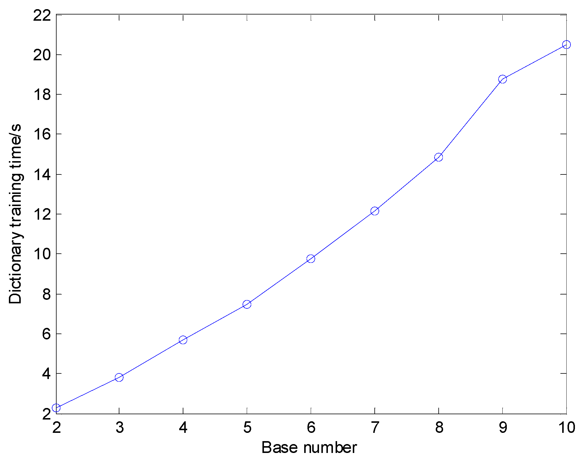
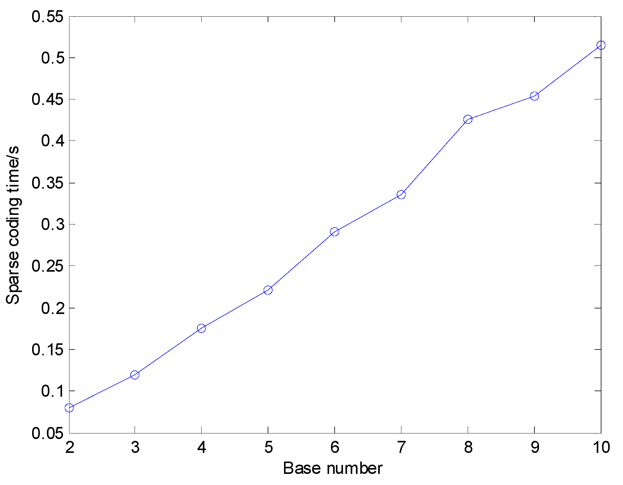
For different K, the dictionary size increased rapidly as K increases, whose classification results and dictionary training time are illustrated in Figure 9 and Figure 10, respectively. The average sparse coding time for one sample using different K is shown in Figure 11. Figure 9 shows that in general the diagnosis accuracy grows with the increasing number of base functions K, yet becomes steady when dictionary size reaches a relatively large value. Nevertheless, Figure 10 and Figure 11 show that the dictionary training time rises quickly if dictionary size is increased and then the time of sparse coding for the training samples and test samples also grows quickly. Therefore, a proper value of K should be selected in addition to considering the diagnosis precision, the computing, and memory consumption must also be taken into account comprehensively. In this paper, K is set to 4.
5.3.3. Diagnosis Results Using Optimized SVM
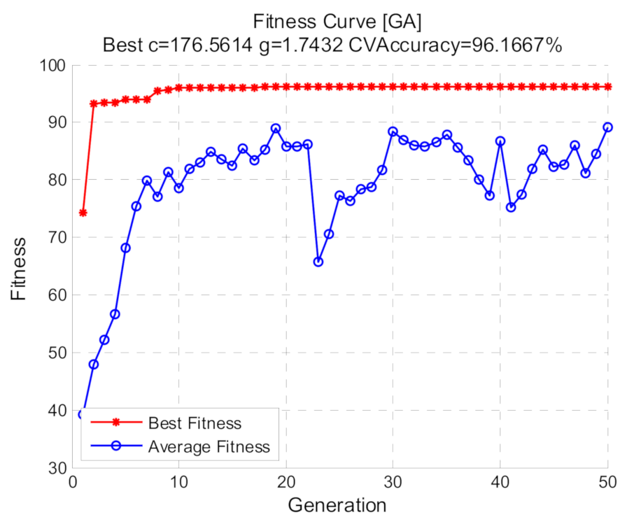
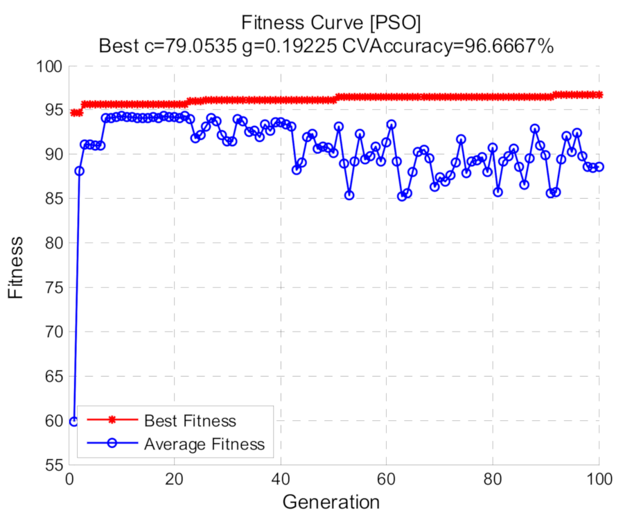
Using shift invariant sparse feature, optimized SVM with three methods including grid search, GA and PSO were respectively conducted. For all the methods, the selection ranges of (c, g) are restricted to 2−10 to 210 and 5-fold cross validation is used. As for grid search, the logarithms of c and g based on 2 are stepped with the step size 1. With regard to GA and PSO, the fitness represents the c ross-validation accuracy and the population size is 20, the max generations are 100. The other parameters of GA including crossover and mutation probability are set to 0.4 and 0.2, respectively, while the other parameters of PSO are: wv = 1, wp = 1, c1 = 1.5 and c2 = 1.7. The result of the grid search is demonstrated in Figure 12, while Figure 13 and Figure 14 demonstrate the fitness curves of GA and PSO, respectively. The figures show that the loops in the GA algorithm are terminated at the 50th generation and based on the training set, the best cross validation accuracies of the three methods corresponding to the best (c, g) are relatively high.
Using the best (c, g), the optimized SVM model is obtained based on the training samples, which can be employed to acquire the category labels of the test set. For LIBSVM, the default values of (c, g) are (1, 1/k) (k denotes data dimension). SVM with default (c, g) was also conducted for comparison with optimized SVM. Table 2 demonstrates the diagnosis results and computation time of different methods. The table indicates that the proposed method based on the shift invariant sparse feature and optimized SVM can effectively distinguish different operating conditions, thus the fault diagnosis of rolling bearings is achieved. Under default parameters (c, g), the diagnosis precision is not high, therefore different parameters of SVM have significant impact on the diagnosis precision and it is necessary to conduct the process of parameter optimization. For the three optimization methods, the PSO method acquires the highest accuracy. Moreover, the computation times of GA and PSO are much longer than grid search so the efficiency of the algorithms needs to be improved. Of course, the classification accuracies and computation times of the optimization algorithms are affected by the parameters set of the algorithms themselves. Generally speaking, when the dataset scale is small, using grid search is sufficient to meet the demand, but if the dataset scale is too large it is better to use GA or PSO algorithm.
6. Conclusions
In this paper, a new fault diagnosis method for rolling bearing based on shift invariant sparse feature and optimized SVM is proposed. The shift invariant sparse feature is applied for extracting shift invariant features of the vibration signals of rolling bearings, which presents the characteristics of periodic recurrence of fault impact. The experiment of rolling bearing fault was carried out and through the analysis of experimental vibration signal, it can be found out that shift invariant sparse feature based on shift invariant K-SVD is very discriminative, which can effectively distinguish different states of rolling bearings. For shift invariant sparse feature based on different methods, l1 norm achieves the highest classification accuracy. The influence of the parameter in shift invariant sparse feature, namely the number of basis functions is also discussed, which shows that the number of basis functions should be set comprehensively considering the diagnosis precision, the computing, and memory consumption. As for optimized SVM, the classification results indicate that parameter optimization is very essential for SVM and optimized SVM using the methods of grid search, GA, or PSO can dramatically improve the classification ability of SVM. With respect to the three methods, although PSO owns the longest running time, it obtains the highest classification accuracy. In future work, combining other effective shift invariant dictionary learning methods to obtain superior sparse features of bearing fault will be explored. For the optimized SVM, improved optimization methods based on GA or PSO can be considered to further enhance the optimization ability.
Author Contributions
Conceptualization, H.Y. and N.W.; methodology, H.Y.; software, H.Y.; validation, X.C., N.W. and H.Y.; formal analysis, N.W.; investigation, H.Y. and N.W.; resources, H.Y. and N.W.; data curation, H.Y.; writing—original draft preparation, H.Y.; writing—review and editing, H.Y. and N.W.; visualization, X.C.; supervision, Y.W.; project administration, H.Y. and N.W.; funding acquisition, H.Y. and N.W. All authors have read and agreed to the published version of the manuscript.
Funding
This research received no external funding.
Data Availability Statement
The data used to support the findings of this study are available from the corresponding author upon request.
Acknowledgments
The research carried out in this paper was supported by the Fundamental Research Funds for the Central Universities (2232019D3-61) as well as the initial research fund for the young teachers of Donghua University.
Conflicts of Interest
The authors declare no conflict of interest.
Notations
| c | penalization factor in SVM |
| c1 | acceleration coefficient that represents the local search ability |
| c2 | acceleration coefficient that represents the global search ability |
| dk | the kth basis function |
| d | basis function |
| D | over-complete dictionary |
| F | shift invariant sparse feature |
| g | the width of RBF kernel in SVM using RBF kernel |
| gbest | the best particle that indicates the global best |
| j | class label |
| K | basis function number |
| L | class number of signals |
| M | the number of maximum absolute values |
| N | population size in PSO |
| p | the length of the long signal x |
| pbesti | the best value of the ith particle that indicates the local best |
| pi | the ith particle |
| q | the length of the basis function |
| r | residual signal |
| r1 | random number uniformly distributed in [0, 1] |
| r2 | random number uniformly distributed in [0, 1] |
| s | sparse coefficient corresponding to the long signal |
| Sk,τ | the sparse coefficient corresponding to the dictionary atom after basis function is translated to time τ and extended |
| t | iteration number |
| T | sparsity prior |
| Tτ | shift operator |
| the operator corresponding to , which can extract a segment with the same length q as the basis function from the long signal and the segment starts at time τ | |
| vi | velocity of the ith particle |
| wv | elastic coefficient for velocity update |
| wp | elastic coefficient for particle update |
| x | long signal |
| X | training set |
| the signal with no contribution from other basis functions | |
| σκ | the set of non-zero elements |
| ε | tolerance error |
References
- Dabov, K.; Foi, A.; Katkovnik, V.; Egiazarian, K. Image Denoising by Sparse 3-D Transform-Domain Collaborative Filtering. IEEE Trans. Image Process. 2007, 16, 2080–2095. [Google Scholar] [CrossRef] [PubMed]
- Zhang, Y.; Zhang, H.; Yu, M.; Kwong, S.; Ho, Y.S. Sparse Representation-Based Video Quality Assessment for Synthesized 3D Videos. IEEE Trans. Image Process. 2020, 29, 509–524. [Google Scholar] [CrossRef] [PubMed]
- Liu, H.Q.; Liu, S.J.; Li, Y.; Li, D.; Truong, T.K. Speech Denoising Based on Group Sparse Representation in the Case of Gaussian Noise. In Proceedings of the 2018 IEEE 23rd International Conference on Digital Signal Processing (DSP), Shanghai, China, 19–21 November 2018. [Google Scholar]
- Zhong, J.; Wang, D.; Guo, J.; Cabrera, D.; Li, C. Theoretical Investigations on Kurtosis and Entropy and Their Improvements for System Health Monitoring. IEEE Trans. Instrum. Meas. 2020, 1–10. [Google Scholar] [CrossRef]
- Yu, F.J.; Zhou, F.X. Classification of Machinery Vibration Signals Based on Group Sparse Representation. J. Vibroeng. 2016, 18, 1540–1554. [Google Scholar] [CrossRef]
- Peng, W.; Wang, D.; Shen, C.Q.; Liu, D.N. Sparse Signal Representations of Bearing Fault Signals for Exhibiting Bearing Fault Features. Shock Vib. 2016. [Google Scholar] [CrossRef] [Green Version]
- Fan, W.; Cai, G.G.; Zhu, Z.K.; Shen, C.Q.; Huang, W.G.; Shang, L. Sparse Representation of Transients in Wavelet Basis and its Application in Gearbox Fault Feature Extraction. Mech. Syst. Signal Process. 2015, 56–57, 230–245. [Google Scholar] [CrossRef]
- Aharon, M.; Elad, M.; Bruckstein, A. K-SVD: An Algorithm for Designing Overcomplete Dictionaries for Sparse Representation. IEEE Trans. Signal Process. 2006, 54, 4311–4322. [Google Scholar] [CrossRef]
- Engan, K.; Aase, S.O.; Husoy, J.H. Multi-Frame Compression: Theory and Design. Signal Process. 2000, 80, 2121–2140. [Google Scholar] [CrossRef]
- Wang, T.; Feng, H.S.; Li, S.; Yang, Y. Medical Image Denoising Using Bilateral Filter and the KSVD Algorithm. In Proceedings of the 2019 3rd International Conference on Machine Vision and Information Technology (CMVIT 2019), Guangzhou, China, 22–24 February 2019; Volume 1229. [Google Scholar] [CrossRef]
- Liu, J.J.; Liu, W.Q.; Ma, S.W.; Wang, M.X.; Li, L.; Chen, G.H. Image-set Based Face Recognition Using K-SVD Dictionary Learning. Int. J. Mach. Learn. Cybern. 2019, 10, 1051–1064. [Google Scholar] [CrossRef]
- Li, S.T.; Ye, W.B.; Liang, H.W.; Pan, X.F.; Lou, X.; Zhao, X.J. K-SVD Based Denoising Algorithm for DoFP Polarization Image Sensors. In Proceedings of the 2018 IEEE International Symposium on Circuits and Systems (ISCAS), Florence, Italy, 27–30 May 2018. [Google Scholar] [CrossRef]
- Zhu, K.P.; Vogel-Heuser, B. Sparse Representation and its Applications in Micro-Milling Condition Monitoring: Noise Separation and Tool Condition Monitoring. Int. J. Adv. Manuf. Technol. 2014, 70, 185–199. [Google Scholar] [CrossRef]
- Zeng, M.; Zhang, W.M.; Chen, Z. Group-Based K-SVD Denoising for Bearing Fault Diagnosis. IEEE Sens. J. 2019, 19, 6335–6343. [Google Scholar] [CrossRef]
- Grosse, R.; Raina, R.; Kwong, H.; Ng, A.Y. Shift-Invariant Sparse Coding for Audio Classification. In Proceedings of the Proceedings of the Twenty-Third Conference on Uncertainty in AI, Vancouver, BC, Canada, 19–22 July 2007; pp. 149–158. [Google Scholar]
- Wohlberg, B. Efficient Algorithms for Convolutional Sparse Representations. IEEE Trans. Image Process. 2016, 25, 301–315. [Google Scholar] [CrossRef]
- Mailhé, B.; Lesage, S.; Bimbot, F.; Vandergheynst, P. Shift-Invariant Dictionary Learning for Sparse Representations: Extending K-SVD. In Proceedings of the 16th European Signal Processing Conference (EUSIPCO’08), Lausanne, Switzerland, 25 August 2008; pp. 1–5. [Google Scholar]
- Liu, H.N.; Liu, C.L.; Huang, Y.X. Adaptive Feature Extraction Using Sparse Coding for Machinery Fault Diagnosis. Mech. Syst. Signal Process. 2011, 25, 558–574. [Google Scholar] [CrossRef]
- Feng, Z.P.; Liang, M. Complex Signal Analysis for Planetary Gearbox Fault Diagnosis via Shift Invariant Dictionary Learning. Measurement 2016, 90, 382–395. [Google Scholar] [CrossRef]
- Tang, H.F.; Chen, J.; Dong, G.M. Sparse Representation Based Latent Components Analysis for Machinery Weak Fault Detection. Mech. Syst. Signal Process. 2014, 46, 373–388. [Google Scholar] [CrossRef]
- Yang, B.Y.; Liu, R.N.; Chen, X.F. Fault Diagnosis for a Wind Turbine Generator Bearing via Sparse Representation and Shift-Invariant K-SVD. IEEE Trans. Ind. Inform. 2017, 13, 1321–1331. [Google Scholar] [CrossRef]
- Ding, J.M. Fault Detection of a Wheelset Bearing in a High-Speed Train Using the Shock-Response Convolutional Sparse-Coding Technique. Measurement 2018, 117, 108–124. [Google Scholar] [CrossRef]
- Li, Q.C.; Ding, X.X.; Huang, W.B.; He, Q.B.; Shao, Y.M. Transient Feature Self-Enhancement via Shift-Invariant Manifold Sparse Learning for Rolling Bearing Health Diagnosis. Measurement 2019, 148. [Google Scholar] [CrossRef]
- Ding, C.C.; Zhao, M.; Lin, J. Sparse Feature Extraction Based on Periodical Convolutional Sparse Representation for Fault Detection of Rotating Machinery. Meas. Sci. Technol. 2021, 32. [Google Scholar] [CrossRef]
- He, L.; Yi, C.; Lin, J.H.; Tan, A.C.C. Fault Detection and Behavior Analysis of Wheelset Bearing Using Adaptive Convolutional Sparse Coding Technique Combined with Bandwidth Optimization. Shock Vib. 2020, 2020. [Google Scholar] [CrossRef]
- Zhou, H.T.; Chen, J.; Dong, G.M.; Wang, R. Detection and Diagnosis of Bearing Faults Using Shift-Invariant Dictionary Learning and Hidden Markov Model. Mech. Syst. Signal Process. 2016, 72–73, 65–79. [Google Scholar] [CrossRef]
- Zhu, K.H.; Chen, L.; Hu, X. Rolling Element Bearing Fault Diagnosis Based on Multi-Scale Global Fuzzy Entropy, Multiple Class Feature Selection and Support Vector Machine. Trans. Inst. Meas. Control 2019, 41, 4013–4022. [Google Scholar] [CrossRef]
- Zhao, H.S.; Gao, Y.F.; Liu, H.H.; Li, L. Fault Diagnosis of Wind Turbine Bearing Based on Stochastic Subspace Identification and Multi-Kernel Support Vector Machine. J. Mod. Power Syst. Clean Energy 2019, 7, 350–356. [Google Scholar] [CrossRef] [Green Version]
- Lu, D.; Qiao, W. Fault Diagnosis for Drivetrain Gearboxes Using PSO-Optimized Multiclass SVM Classifier. In Proceedings of the 2014 IEEE PES General Meeting | Conference & Exposition, National Harbor, MD, USA, 27–31 July 2014; pp. 1–5. [Google Scholar]
- Wang, C.; Jia, L.M.; Li, X.F. Fault Diagnosis Method for the Train Axle Box Bearing Based on KPCA and GA-SVM. Appl. Mech. Mater. 2014, 441, 376–379. [Google Scholar] [CrossRef]
- Long, J.; Mou, J.; Zhang, L.; Zhang, S.; Li, C. Attitude Data-Based Deep Hybrid Learning Architecture for Intelligent Fault Diagnosis of Multi-Joint Industrial Robots. J. Manuf. Syst. 2020. [Google Scholar] [CrossRef]
- Malik, H.; Pandya, Y.; Parashar, A.; Sharma, R. Feature Extraction Using EMD and Classifier Through Artificial Neural Networks for Gearbox Fault Diagnosis. Appl. Artif. Intell. Tech. Eng. 2019, 697, 309–317. [Google Scholar] [CrossRef]
- Wu, Q.E.; Guo, Y.H.; Chen, H.; Qiang, X.L.; Wang, W. Establishment of a Deep Learning Network Based on Feature Extraction and its Application in Gearbox Fault Diagnosis. Artif. Intell. Rev. 2019, 52, 125–149. [Google Scholar] [CrossRef]
- Vapnik, V.N. The Nature of Statistical Learning Theory; Springer: Berlin, Germany, 1995. [Google Scholar]
- Kennedy, J.; Eberhart, R. Particle Swarm Optimization. In Proceedings of the IEEE International Conference on Neural Networks, Perth, WA, Australia, 27 November–1 December 1995; pp. 1942–1948. [Google Scholar]
- Houck, C.R.; Joines, J.A.; Kay, M.G. A Genetic Algorithm for Function Optimization: A MATLAB implementation. NCSU 1998, 22. [Google Scholar]
- Long, J.Y.; Sun, Z.Z.; Panos, M.P.; Hong, Y.; Zhang, S.H.; Li, C. A Hybrid Multi-Objective Genetic Local Search Algorithm for the Prize-Collecting Vehicle Routing Problem. Inform. Sci. 2019, 478, 40–61. [Google Scholar] [CrossRef]
- Krstulovic, S.; Gribonval, R. MPTK: Matching Pursuit Made Tractable. In Proceedings of the 2006 IEEE International Conference on Acoustics Speech and Signal Processing Proceedings, Toulouse, France, 14–19 May 2006; pp. 496–499. [Google Scholar]
- Chang, C.-C.; Lin, C.-J. LIBSVM: A Library for Support Vector Machines. ACM Trans. Intell. Syst. Technol. 2011, 2, 1–27. [Google Scholar] [CrossRef]
Figure 1.
Diagram of the proposed method.

Figure 2.
The test rig.

Figure 3.
Vibration signals corresponding to different running statuses: (a) Normal; (b) inner race fault; (c) rolling element fault; (d) outer race fault.
Figure 3.
Vibration signals corresponding to different running statuses: (a) Normal; (b) inner race fault; (c) rolling element fault; (d) outer race fault.

Figure 4.
The learned basis functions corresponding to four running states: (a1–a4) normal; (b1–b4) inner race fault; (c1–c4) rolling element fault; (d1–d4) outer race fault.
Figure 4.
The learned basis functions corresponding to four running states: (a1–a4) normal; (b1–b4) inner race fault; (c1–c4) rolling element fault; (d1–d4) outer race fault.

Figure 5.
Shift invariant sparse coefficients with respect to different running statuses: (a) normal; (b) inner race fault; (c) rolling element fault; (d) outer race fault.
Figure 5.
Shift invariant sparse coefficients with respect to different running statuses: (a) normal; (b) inner race fault; (c) rolling element fault; (d) outer race fault.

Figure 6.
Shift invariant sparse feature of a test sample with respect to different running statuses: (a) normal; (b) inner race fault; (c) rolling element fault; (d) outer race fault.
Figure 6.
Shift invariant sparse feature of a test sample with respect to different running statuses: (a) normal; (b) inner race fault; (c) rolling element fault; (d) outer race fault.

Figure 7.
Sum of shift invariant sparse feature of all test samples with respect to different running statuses: (a) normal; (b) inner race fault; (c) rolling element fault; (d) outer race fault.
Figure 7.
Sum of shift invariant sparse feature of all test samples with respect to different running statuses: (a) normal; (b) inner race fault; (c) rolling element fault; (d) outer race fault.

Figure 8.
Diagnosis results in detail.

Figure 9.
The classification result of shift invariant sparse feature with different K.

Figure 10.
Dictionary training time using different K.

Figure 11.
Average sparse coding time using different K.

Figure 12.
Optimized SVM using grid search.

Figure 13.
Fitness curve with GA.

Figure 14.
Fitness curve with PSO.


Table 1.
The diagnosis results using different feature and standard SVM (%).
| Max | 2-Max | 3-Max | L1 | L2 |
|---|---|---|---|---|
| 89.7 | 90.0 | 90.3 | 93.3 | 93.0 |
Table 2.
The classification result with different parameters (%).
| Default | Grid Search | GA | PSO | |
|---|---|---|---|---|
| Normal | 97.3 | 98.7 | 98.0 | 98.0 |
| IRF | 94.7 | 96.7 | 97.3 | 96.7 |
| REF | 88.7 | 92.0 | 90.7 | 93.3 |
| ORF | 91.3 | 96.7 | 96.7 | 97.3 |
| Average | 93.0 | 96.0 | 95.7 | 96.3 |
| Time/s | 0.1976 | 57.3465 | 81.7135 | 112.4451 |
Publisher’s Note: MDPI stays neutral with regard to jurisdictional claims in published maps and institutional affiliations. |
© 2021 by the authors. Licensee MDPI, Basel, Switzerland. This article is an open access article distributed under the terms and conditions of the Creative Commons Attribution (CC BY) license (https://creativecommons.org/licenses/by/4.0/).
Share and Cite
MDPI and ACS Style
Yuan, H.; Wu, N.; Chen, X.; Wang, Y. Fault Diagnosis of Rolling Bearing Based on Shift Invariant Sparse Feature and Optimized Support Vector Machine. Machines 2021, 9, 98. https://0-doi-org.brum.beds.ac.uk/10.3390/machines9050098
AMA Style
Yuan H, Wu N, Chen X, Wang Y. Fault Diagnosis of Rolling Bearing Based on Shift Invariant Sparse Feature and Optimized Support Vector Machine. Machines. 2021; 9(5):98. https://0-doi-org.brum.beds.ac.uk/10.3390/machines9050098
Chicago/Turabian StyleYuan, Haodong, Nailong Wu, Xinyuan Chen, and Yueying Wang. 2021. "Fault Diagnosis of Rolling Bearing Based on Shift Invariant Sparse Feature and Optimized Support Vector Machine" Machines 9, no. 5: 98. https://0-doi-org.brum.beds.ac.uk/10.3390/machines9050098
Note that from the first issue of 2016, this journal uses article numbers instead of page numbers. See further details here.