
Ten Fast Transfer Learning Models for Carotid Ultrasound Plaque Tissue Characterization in Augmentation Framework Embedded with Heatmaps for Stroke Risk Stratification

 , , , ,
  ,
,
Abstract
:1. Introduction
2. Literature Survey
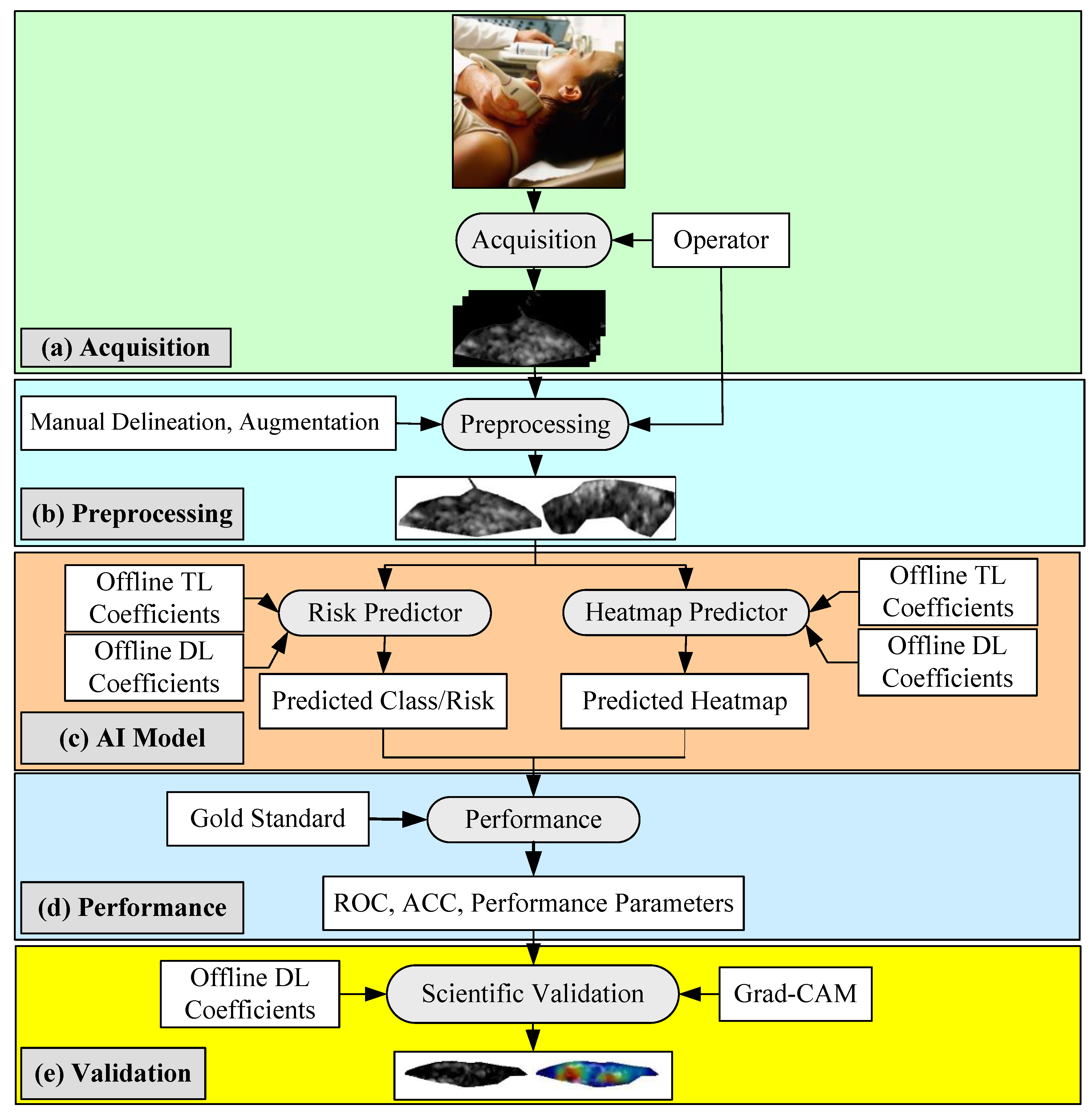
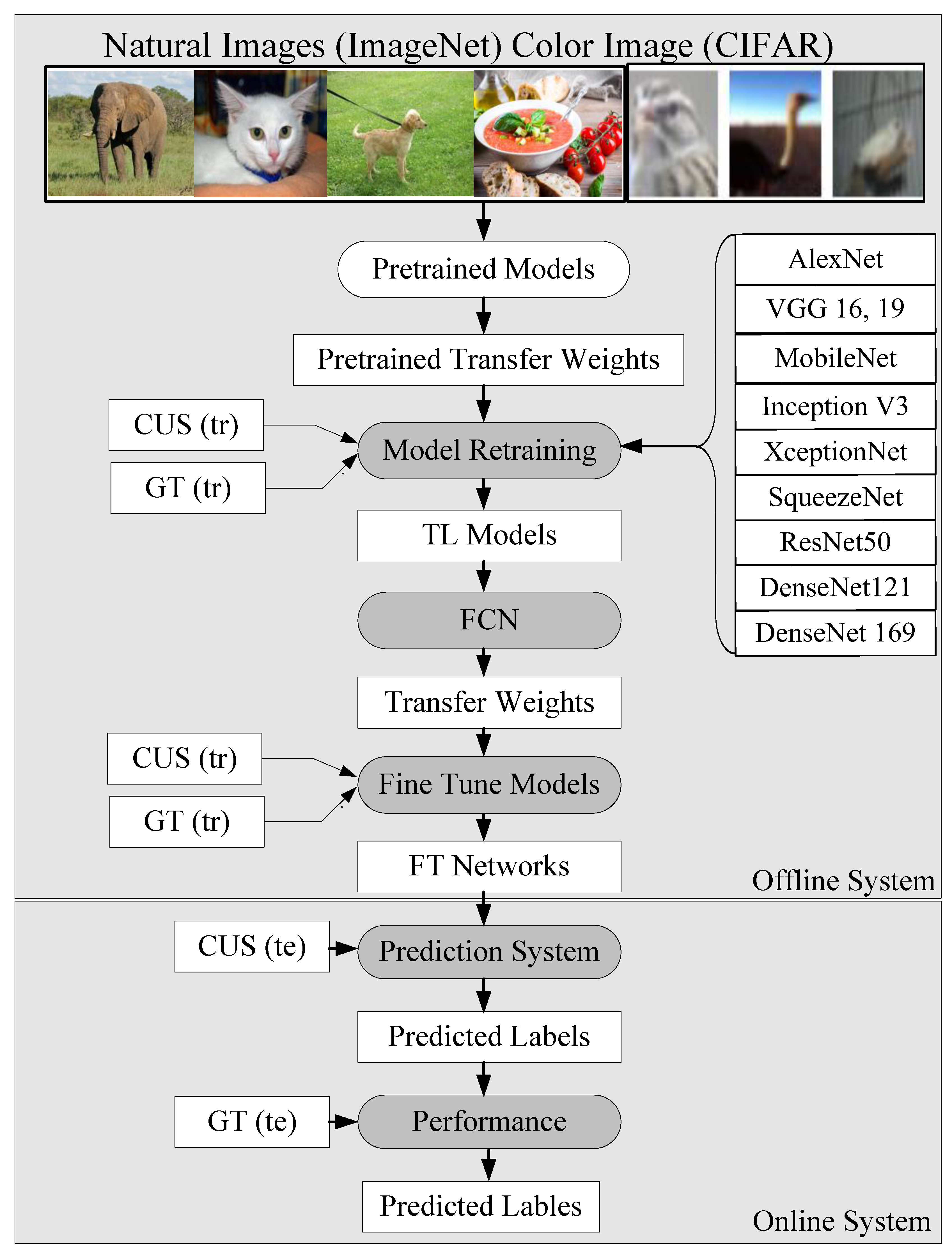
3. Methodology
3.1. Patient Demographics
3.2. Ultrasound Data Acquisition and Pre-Processing
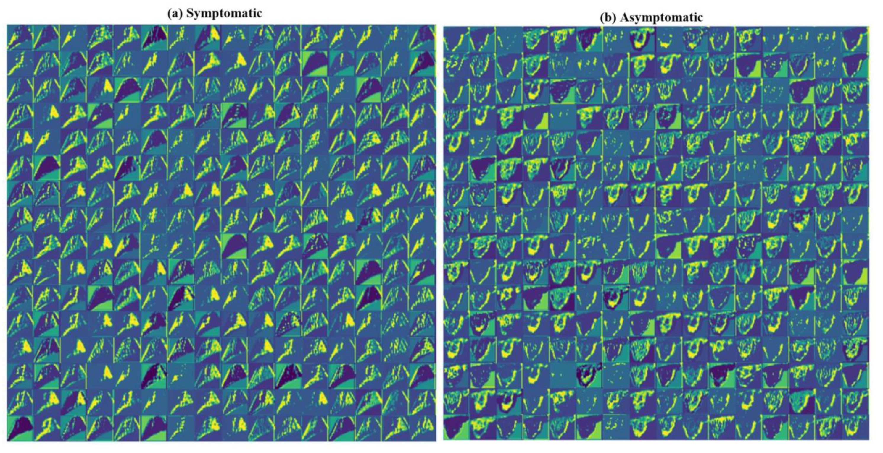
3.3. Augmentation
3.4. Transfer Learning
3.4.1. VGG-16 and VGG-19
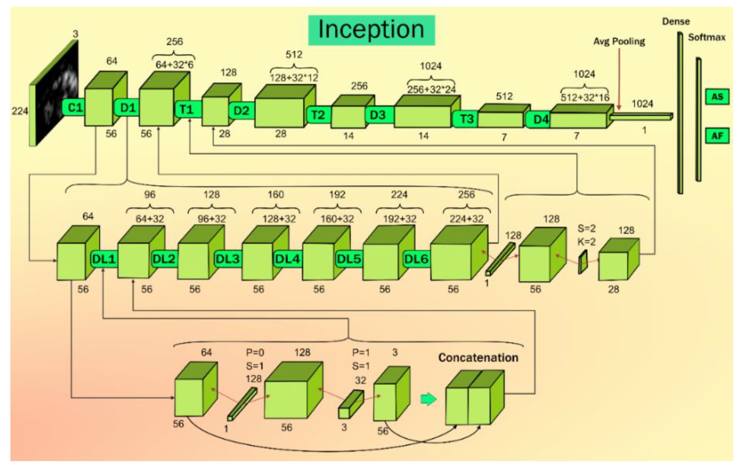
3.4.2. InceptionV3
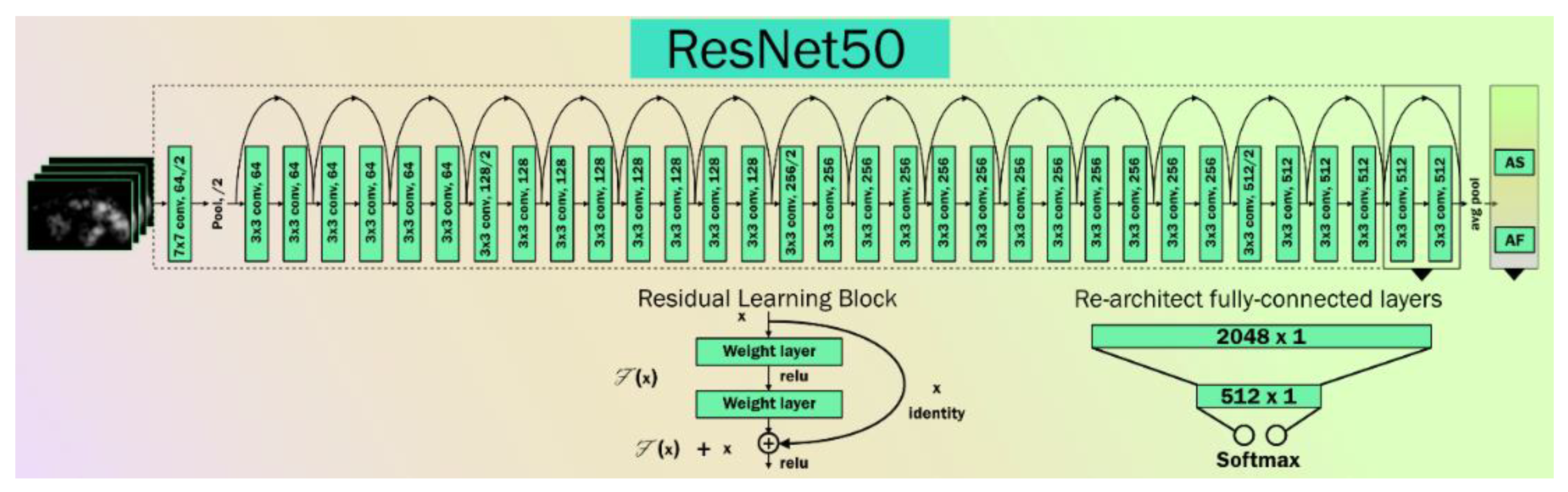
3.4.3. ResNet
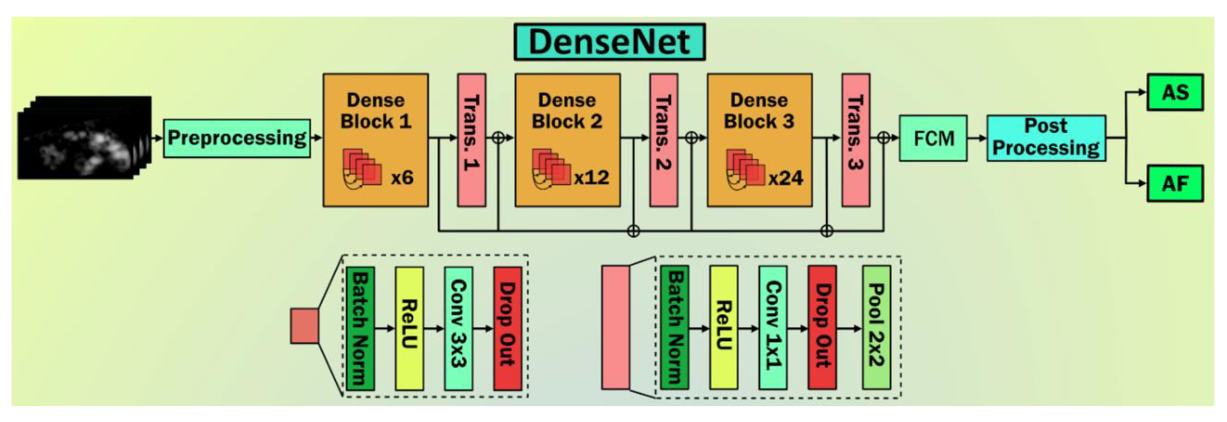
3.4.4. DenseNet
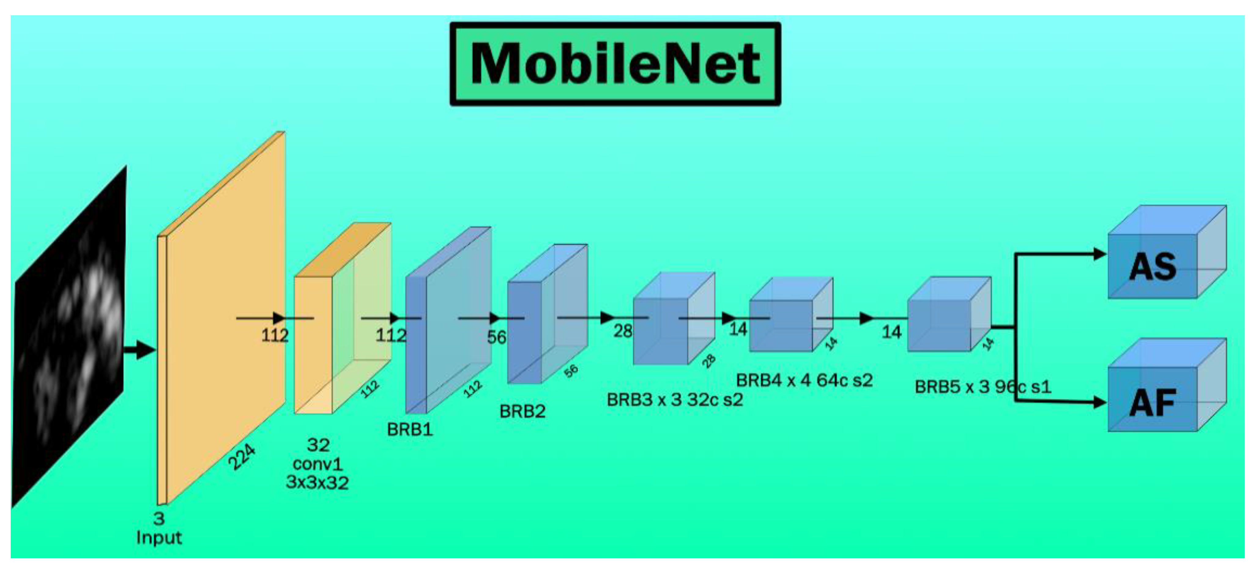
3.4.5. MobileNet
3.4.6. XceptionNet
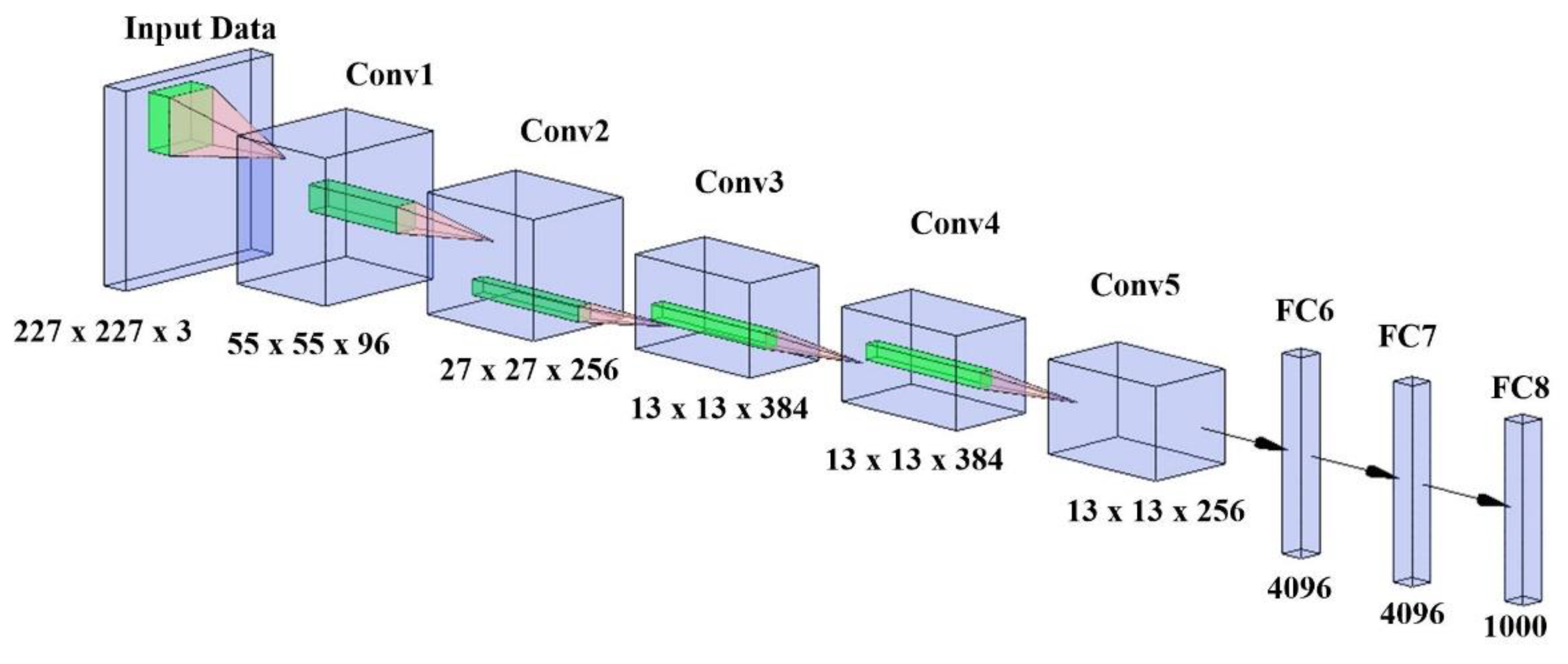
3.4.7. AlexNet
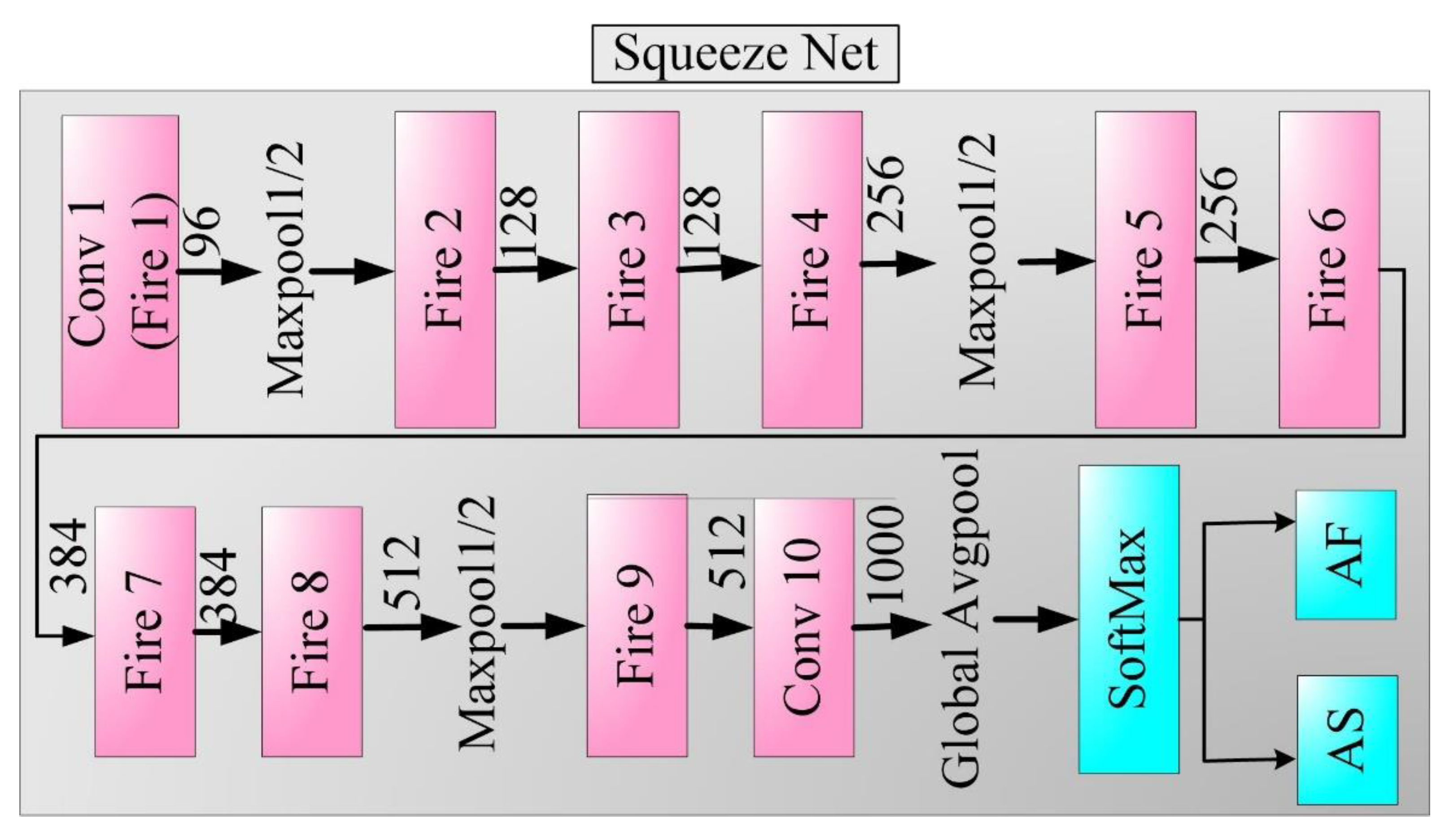
3.4.8. SqueezeNet
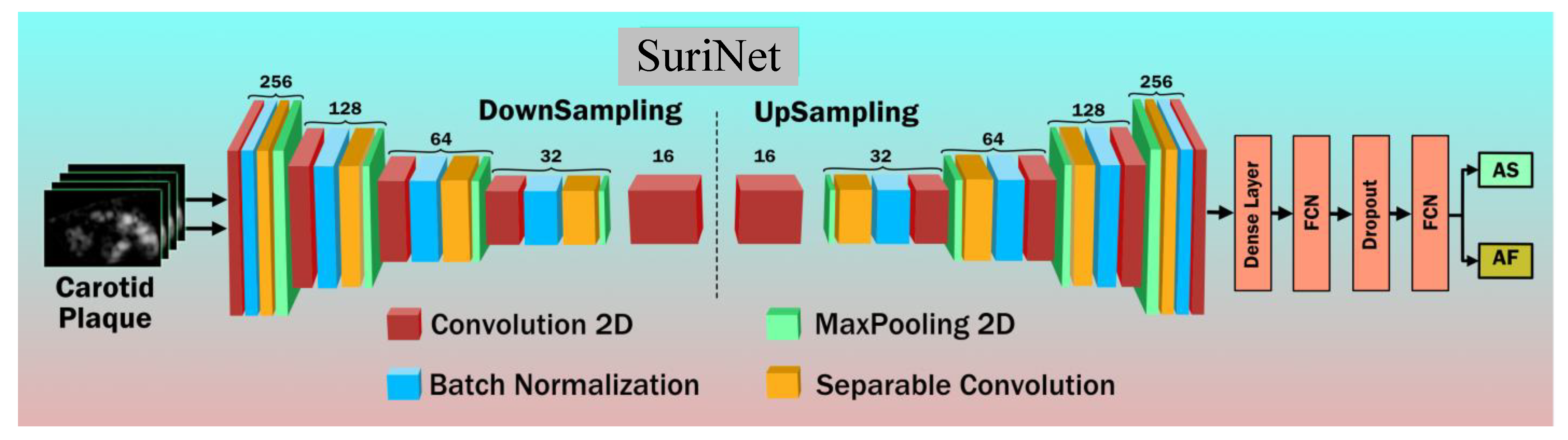
3.5. Deep Learning Architecture: SuriNet
3.6. Experimental Protocol
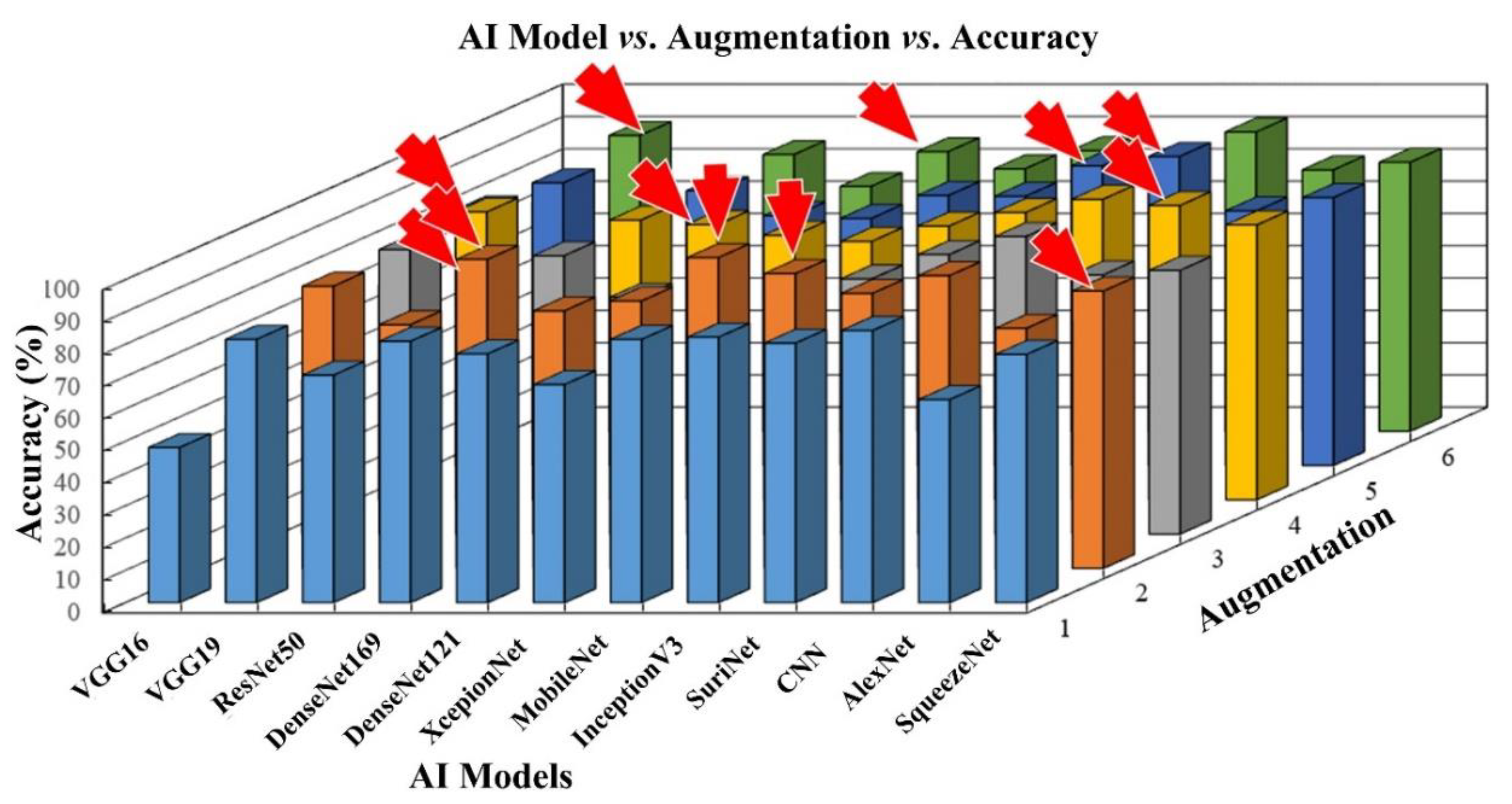
3.6.1. Accuracy Bar Charts for Each Cohort Corresponding to All AI Models
3.6.2. Performance Analysis and Visualization of SuriNet
4. Results
4.1. 3D Optimization of TL Architectures and Benchmarking against CNN
4.2. 3D Optimization of SuriNet
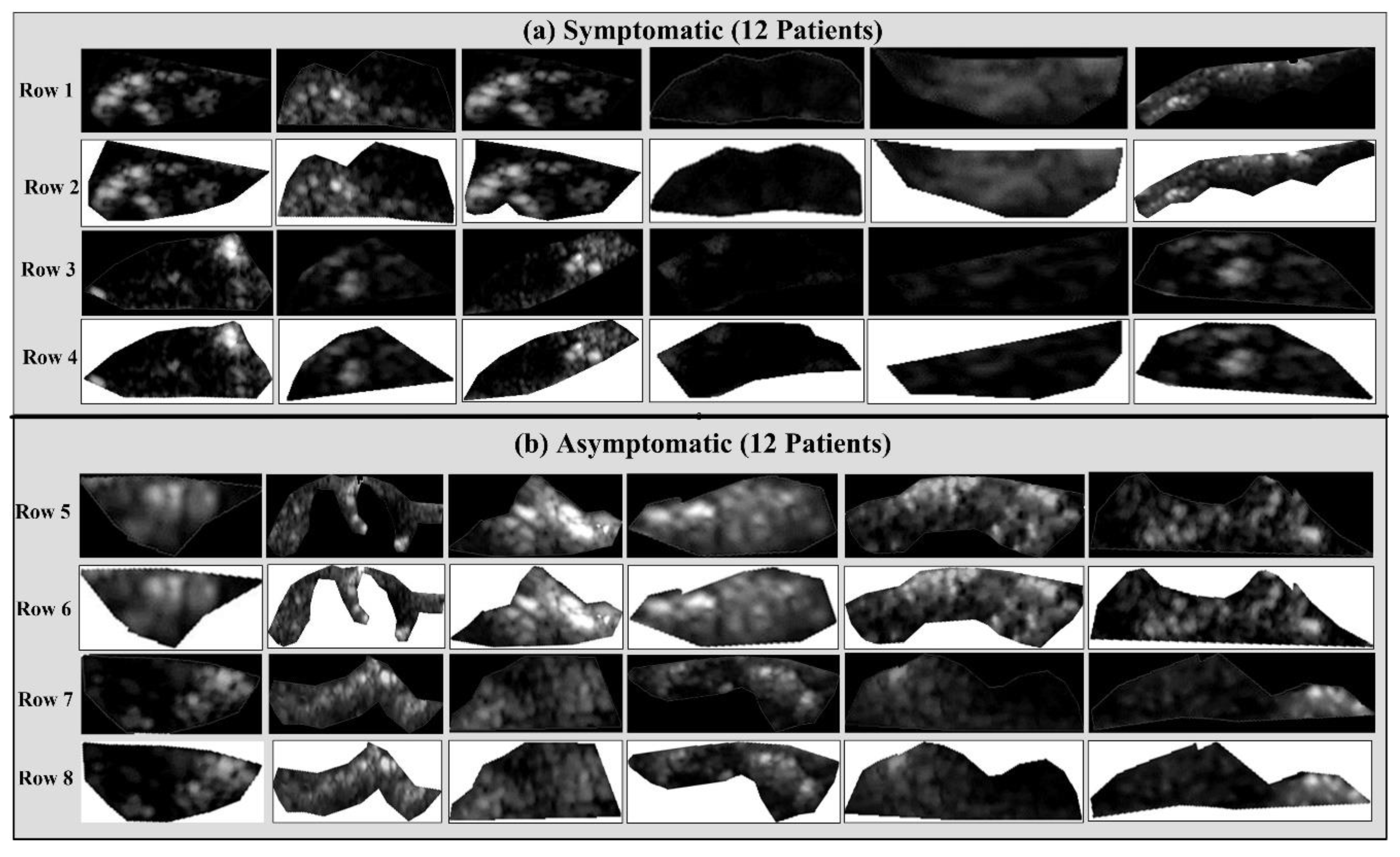
4.3. Visualization of the SuriNet
5. Performance Evaluation
5.1. Power Analysis
5.2. Ranking of AI Models
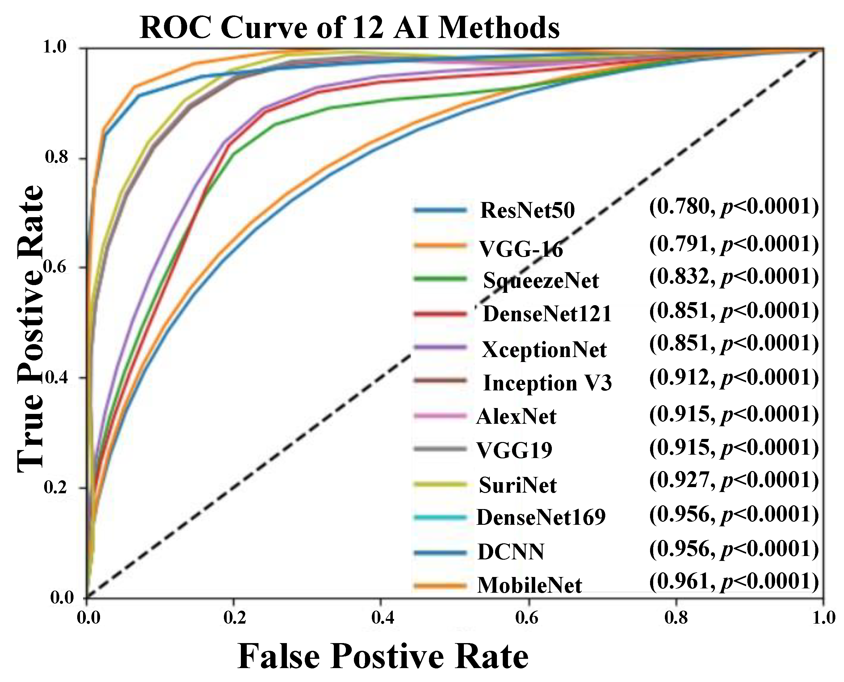
5.3. AUC-ROC Analysis
6. Scientific Validation versus Clinical Validation
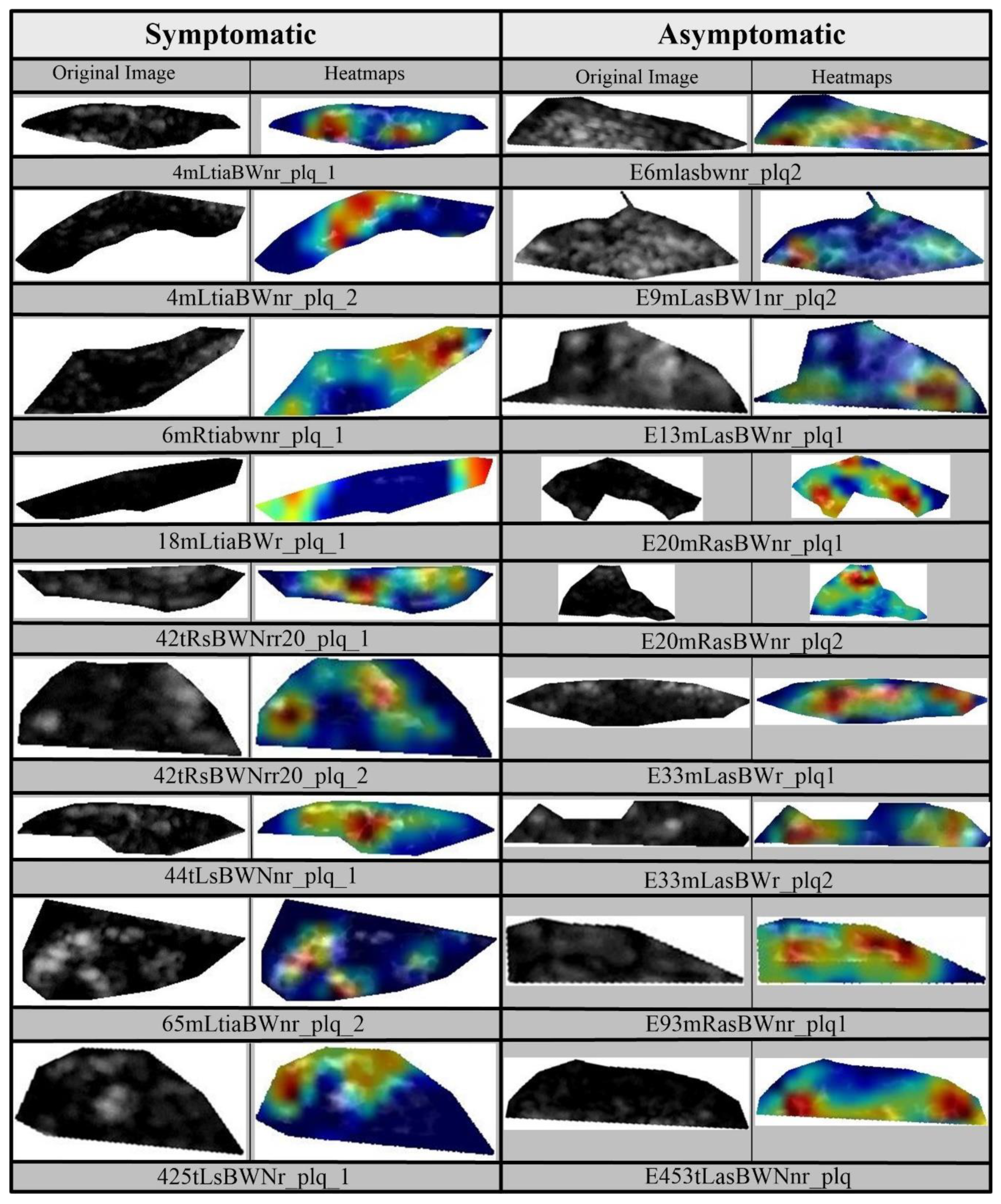
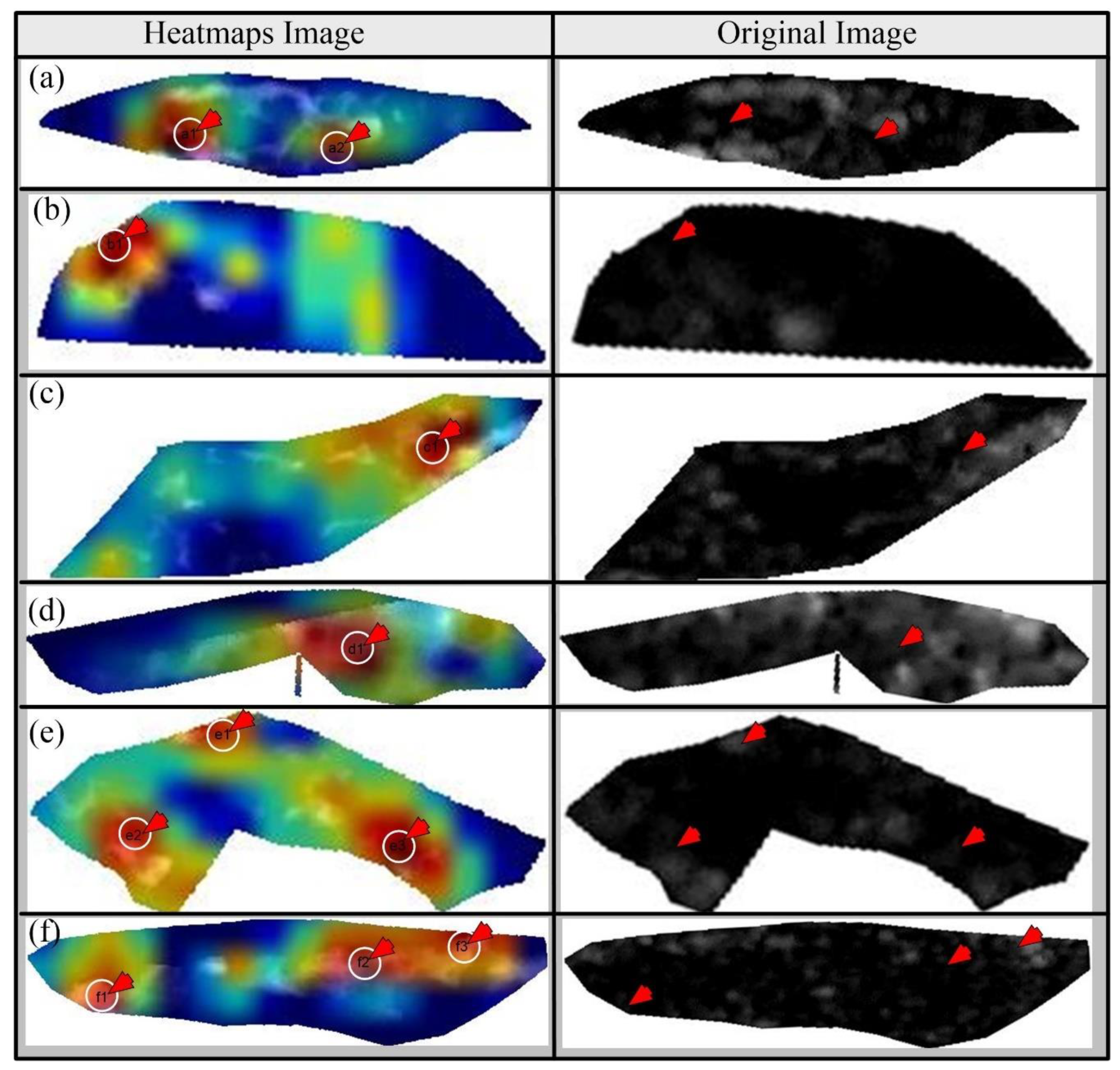
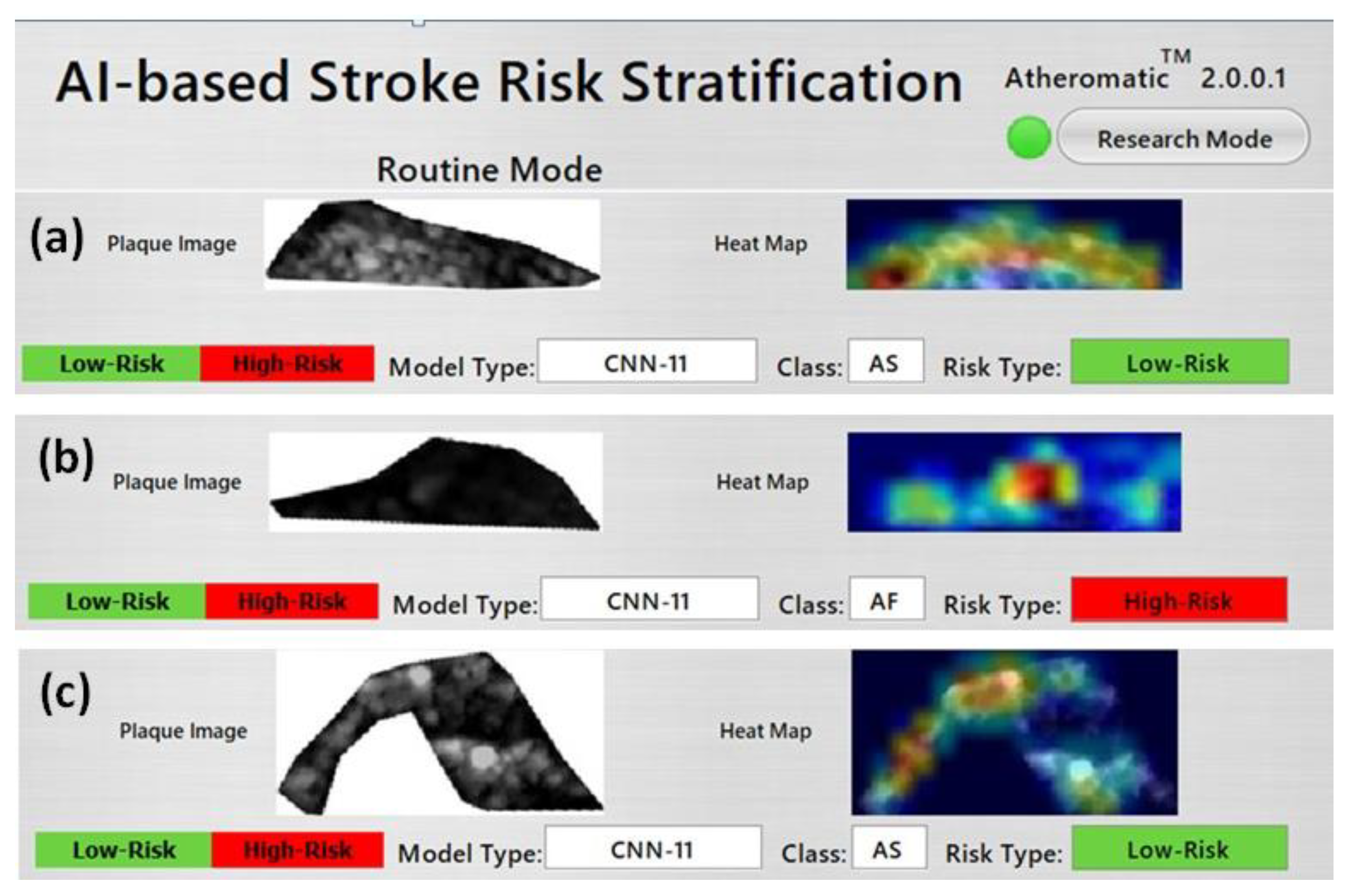
6.1. Scientific Validation Using Heatmaps
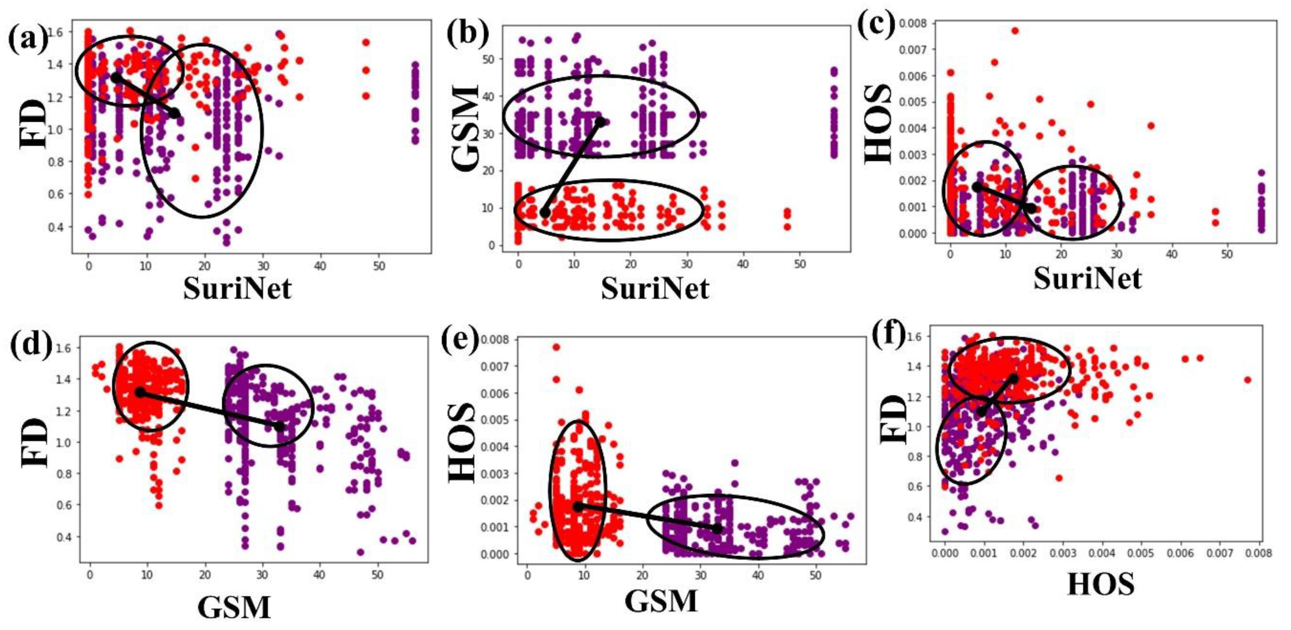
6.2. Correlation Analysis
7. Discussion
7.1. Benchmarking
7.2. Comparison of TL Models
7.3. Advantages of TL Models
7.4. GUI Design
7.5. Strengths/Weakness/Extensions
8. Conclusions
Author Contributions
Funding
Institutional Review Board Statement
Informed Consent Statement
Conflicts of Interest
Abbreviations
| Symbol | Abbreviation |
| Acc | Accuracy |
| AF | Amaurosis fugax |
| AI | Artificial intelligence |
| APSI | Atheromatic plaque separation index |
| Asym | Asymptomatic plaque |
| AUC | Area-under-the-curve |
| CAD | Computer-aided diagnostic |
| CT | Computed tomography |
| CV | Cross-validation |
| CVD | Cardiovascular disease |
| DCNN | Deep convolutional neural network |
| DL | Deep learning |
| DOR | Diagnostics odds ratio |
| DWT | Discrete wavelets transform |
| DY | Diagnostic yield |
| EAI | Enhanced activity index |
| ED | Euclidean distance |
| FC, FCN | Fully connected network |
| FD | Fractal dimension |
| FN | Fine-tune networks |
| GLDS | Gray level difference statistic |
| Grad-Cam | Gradient-weighted class activation map |
| GSM | Greyscale median |
| ICA | Internal carotid artery |
| IV3 | Inception V3 |
| k-NN | K-nearest neighbor |
| LOPO | Leave-one-participant-out |
| MFS | Mean feature strength |
| ML | Machine learning |
| MRI | Magnetic resonance imaging |
| MUV | M-mode ultrasound videos |
| PTC | Plaque tissue characterization |
| ReLu | Rectified linear unit |
| RMM | Rayleigh mixture model |
| ROC | Receiver operating characteristic curve |
| ROI | Region-of-interest |
| SACI | Symptomatic and asymptomatic carotid index |
| SGLD | Spatial gray level dependence matrices |
| SOM | Self-organizing map |
| SVM | Support vector machine |
| sym | Symptomatic plaque |
| TL | Transfer learning |
| US | Ultrasound |
| USA | United States of America |
| VGG | Visual geometric group |
| WHO | World Health Organization |
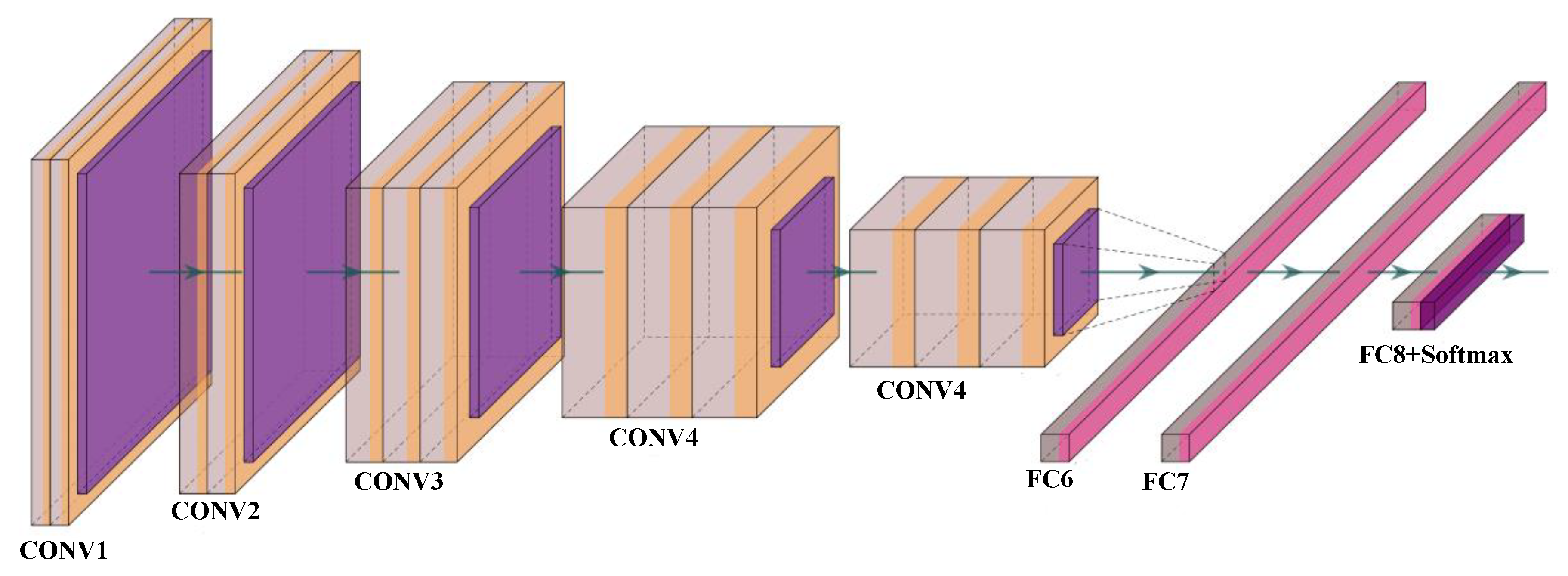
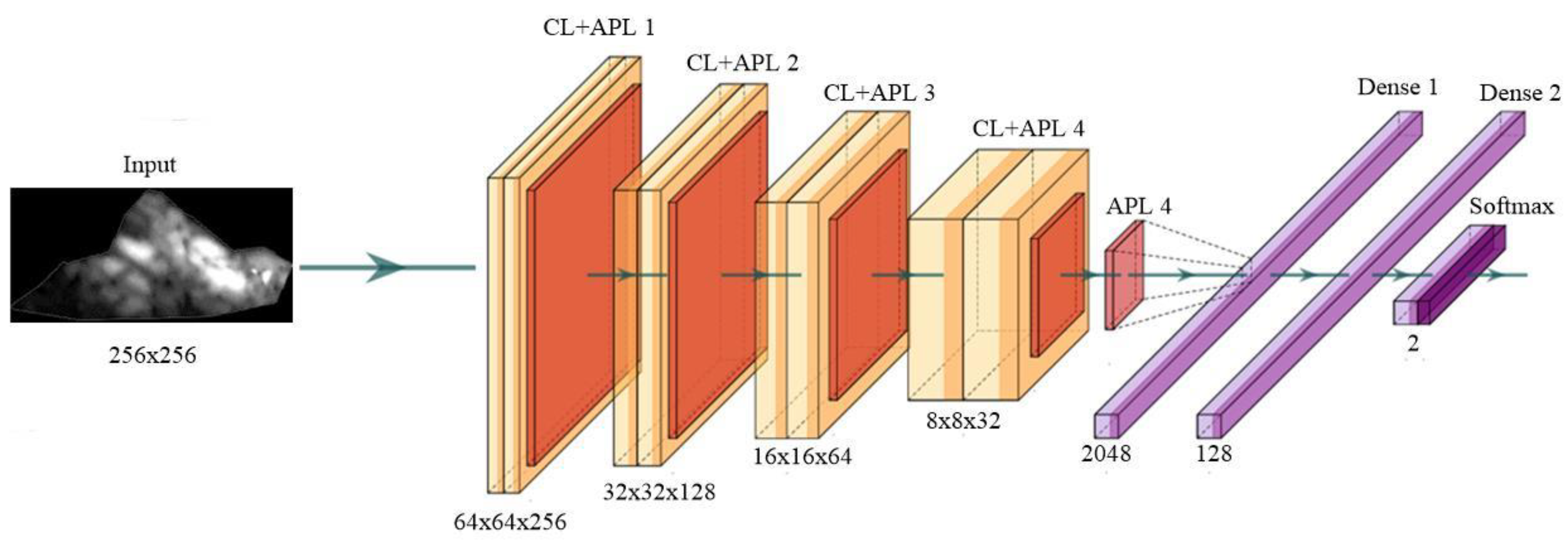
Appendix A. CNN Architecture
Appendix A.1. Deep Convolutional Neural Network Architecture

Appendix A.2. 3-D Optimization of Deep Convolutional Neural Network Architecture

| R# | Column1 | Column2 | Column3 | Column4 |
|---|---|---|---|---|
| DCNN Type | Convolution 2D Layers | Average Pooling Layers | Dense Layers | |
| R1 | DCNN5 | 1 | 1 | 3 |
| R2 | DCNN7 | 2 | 2 | 3 |
| R3 | DCNN9 | 3 | 3 | 3 |
| R4 | DCNN11 | 4 | 4 | 3 |
| R5 | DCNN13 | 5 | 5 | 3 |
| R6 | DCNN15 | 6 | 6 | 3 |
Appendix B. Grading Scheme for Ranking TL Systems
| SN | Attribute | High Grade (4–5) | Medium Grade (3–2) | Low Grade (1–0) |
|---|---|---|---|---|
| 1 | Optimization | High Aug (>5) | Avg Aug (<5 and ≥3) | Low Aug (<3) |
| 2 | Accuracy | >95 | >85 to <95 | <85 |
| 3 | False Positive Rate | <0.1 | >0.1 to <0.2 | >0.2 |
| 4 | F1 Score | >0.9 | >0.8 and <0.9 | <0.8 |
| 5 | Sensitivity | >0.9 | >0.8 and <0.9 | <0.8 |
| 6 | Specificity | >0.9 | >0.8 and <0.9 | <0.8 |
| 7 | Data Size | >1600 | >800 and <1600 | ≤800 |
| 8 | DOR | >300 | >150 and <300 | <150 |
| 9 | Training Time | <24 h | >24 h and <30 | >30 h |
| 10 | Memory | ≤15 MB | >15 MB and <20 MB | >20 MB |
| 11 | AUC | >0.95 | >0.85 to <0.95 | <0.85 |
References
- Benjamin, E.J.; Muntner, P.; Bittencourt, M.S. Heart disease and stroke statistics-2019 update: A report from the American Heart Association. Circulation 2019, 139, e56–e528. [Google Scholar] [CrossRef]
- Virani, S.S.; Alonso, A.; Benjamin, E.J.; Bittencourt, M.S.; Callaway, C.W.; Carson, A.P.; Chamberlain, A.M.; Chang, A.R.; Cheng, S.; Delling, F.N. Heart disease and stroke statistics—2020 update: A report from the American Heart Association. Circulation 2020, 141, e139–e596. [Google Scholar] [CrossRef]
- Suri, J.S.; Kathuria, C.; Molinari, F. Atherosclerosis Disease Management; Springer Science & Business Media: Berlin/Heidelberg, Germany, 2010. [Google Scholar]
- Nicolaides, A.; Beach, K.W.; Kyriacou, E.; Pattichis, C.S. Ultrasound and Carotid Bifurcation Atherosclerosis; Springer Science & Business Media: Berlin/Heidelberg, Germany, 2011. [Google Scholar]
- Kakkos, S.K.; Griffin, M.B.; Nicolaides, A.N.; Kyriacou, E.; Sabetai, M.M.; Tegos, T.; Makris, G.C.; Thomas, D.J.; Geroulakos, G. The size of juxtaluminal hypoechoic area in ultrasound images of asymptomatic carotid plaques predicts the occurrence of stroke. J. Vasc. Surg. 2013, 57, 609–618.e601. [Google Scholar] [CrossRef] [Green Version]
- Bentzon, J.F.; Otsuka, F.; Virmani, R.; Falk, E. Mechanisms of plaque formation and rupture. Circ. Res. 2014, 114, 1852–1866. [Google Scholar] [CrossRef]
- Cuadrado-Godia, E.; Dwivedi, P.; Sharma, S.; Santiago, A.O.; Gonzalez, J.R.; Balcells, M.; Laird, J.; Turk, M.; Suri, H.S.; Nicolaides, A. cerebral small vessel disease: A review focusing on pathophysiology, biomarkers, and machine learning strategies. J. Stroke 2018, 20, 302. [Google Scholar] [CrossRef]
- Saba, L.; Gao, H.; Raz, E.; Sree, S.V.; Mannelli, L.; Tallapally, N.; Molinari, F.; Bassareo, P.P.; Acharya, U.R.; Poppert, H. Semiautomated analysis of carotid artery wall thickness in MRI. J. Magn. Reson. Imaging 2014, 39, 1457–1467. [Google Scholar] [CrossRef]
- Saba, L.; Suri, J.S. Multi-Detector CT Imaging: Principles, Head, Neck, and Vascular Systems; CRC Press: Boca Raton, FL, USA, 2013; Volume 1. [Google Scholar]
- Seabra, J.; Sanches, J. Ultrasound Imaging: Advances and Applications; Springer: Berlin/Heidelberg, Germany, 2012. [Google Scholar]
- Sanches, J.M.; Laine, A.F.; Suri, J.S. Ultrasound Imaging; Springer: Berlin/Heidelberg, Germany, 2012. [Google Scholar]
- Londhe, N.D.; Suri, J.S. Superharmonic imaging for medical ultrasound: A review. J. Med. Syst. 2016, 40, 279. [Google Scholar] [CrossRef]
- Hussain, M.A.; Saposnik, G.; Raju, S.; Salata, K.; Mamdani, M.; Tu, J.V.; Bhatt, D.L.; Verma, S.; Al-Omran, M. Association between statin use and cardiovascular events after carotid artery revascularization. J. Am. Heart Assoc. 2018, 7, e009745. [Google Scholar] [CrossRef]
- Acharya, U.R.; Sree, S.V.; Ribeiro, R.; Krishnamurthi, G.; Marinho, R.T.; Sanches, J.; Suri, J.S. Data mining framework for fatty liver disease classification in ultrasound: A hybrid feature extraction paradigm. Med. Phys. 2012, 39, 4255–4264. [Google Scholar] [CrossRef] [Green Version]
- Saba, L.; Dey, N.; Ashour, A.S.; Samanta, S.; Nath, S.S.; Chakraborty, S.; Sanches, J.; Kumar, D.; Marinho, R.; Suri, J.S. Automated stratification of liver disease in ultrasound: An online accurate feature classification paradigm. Comput. Methods Programs Biomed. 2016, 130, 118–134. [Google Scholar] [CrossRef]
- Acharya, U.R.; Swapna, G.; Sree, S.V.; Molinari, F.; Gupta, S.; Bardales, R.H.; Witkowska, A.; Suri, J.S. A review on ultrasound-based thyroid cancer tissue characterization and automated classification. Technol. Cancer Res. Treat. 2014, 13, 289–301. [Google Scholar] [CrossRef] [Green Version]
- Acharya, U.; Vinitha Sree, S.; Mookiah, M.; Yantri, R.; Molinari, F.; Zieleźnik, W.; Małyszek-Tumidajewicz, J.; Stępień, B.; Bardales, R.; Witkowska, A. Diagnosis of Hashimoto’s thyroiditis in ultrasound using tissue characterization and pixel classification. Proc. Inst. Mech. Eng. Part H. J. Eng. Med. 2013, 227, 788–798. [Google Scholar] [CrossRef]
- Acharya, U.R.; Sree, S.V.; Krishnan, M.M.R.; Molinari, F.; Garberoglio, R.; Suri, J.S. Non-invasive automated 3D thyroid lesion classification in ultrasound: A class of ThyroScan™ systems. Ultrasonics 2012, 52, 508–520. [Google Scholar] [CrossRef]
- Pareek, G.; Acharya, U.R.; Sree, S.V.; Swapna, G.; Yantri, R.; Martis, R.J.; Saba, L.; Krishnamurthi, G.; Mallarini, G.; El-Baz, A. Prostate tissue characterization/classification in 144 patient population using wavelet and higher order spectra features from transrectal ultrasound images. Technol. Cancer Res. Treat. 2013, 12, 545–557. [Google Scholar] [CrossRef]
- McClure, P.; Elnakib, A.; El-Ghar, M.A.; Khalifa, F.; Soliman, A.; El-Diasty, T.; Suri, J.S.; Elmaghraby, A.; El-Baz, A. In-vitro and in-vivo diagnostic techniques for prostate cancer: A review. J. Biomed. Nanotechnol. 2014, 10, 2747–2777. [Google Scholar] [CrossRef]
- Acharya, U.R.; Sree, S.V.; Kulshreshtha, S.; Molinari, F.; Koh, J.E.W.; Saba, L.; Suri, J.S. GyneScan: An improved online paradigm for screening of ovarian cancer via tissue characterization. Technol. Cancer Res. Treat. 2014, 13, 529–539. [Google Scholar] [CrossRef] [Green Version]
- Shrivastava, V.K.; Londhe, N.D.; Sonawane, R.S.; Suri, J.S. Computer-aided diagnosis of psoriasis skin images with HOS, texture and color features: A first comparative study of its kind. Comput. Methods Programs Biomed. 2016, 126, 98–109. [Google Scholar] [CrossRef]
- Shrivastava, V.K.; Londhe, N.D.; Sonawane, R.S.; Suri, J.S. A novel and robust Bayesian approach for segmentation of psoriasis lesions and its risk stratification. Comput. Methods Programs Biomed. 2017, 150, 9–22. [Google Scholar] [CrossRef]
- Kaur, R.; GholamHosseini, H.; Sinha, R. Deep Learning in Medical Applications: Lesion Segmentation in Skin Cancer Images Using Modified and Improved Encoder-Decoder Architecture. Geom. Vis. 2021, 1386, 39. [Google Scholar]
- Sarker, M.M.K.; Rashwan, H.A.; Akram, F.; Singh, V.K.; Banu, S.F.; Chowdhury, F.U.; Choudhury, K.A.; Chambon, S.; Radeva, P.; Puig, D. SLSNet: Skin lesion segmentation using a lightweight generative adversarial network. Expert Syst. Appl. 2021, 115433. [Google Scholar] [CrossRef]
- Maniruzzaman, M.; Kumar, N.; Abedin, M.M.; Islam, M.S.; Suri, H.S.; El-Baz, A.S.; Suri, J.S. Comparative approaches for classification of diabetes mellitus data: Machine learning paradigm. Comput. Methods Programs Biomed. 2017, 152, 23–34. [Google Scholar] [CrossRef]
- Maniruzzaman, M.; Rahman, M.J.; Al-MehediHasan, M.; Suri, H.S.; Abedin, M.M.; El-Baz, A.; Suri, J.S. Accurate diabetes risk stratification using machine learning: Role of missing value and outliers. J. Med. Syst. 2018, 42, 92. [Google Scholar] [CrossRef] [Green Version]
- Acharya, U.R.; Sree, S.V.; Krishnan, M.M.R.; Krishnananda, N.; Ranjan, S.; Umesh, P.; Suri, J.S. Automated classification of patients with coronary artery disease using grayscale features from left ventricle echocardiographic images. Comput. Methods Programs Biomed. 2013, 112, 624–632. [Google Scholar] [CrossRef]
- Acharya, U.R.; Mookiah, M.R.; Vinitha Sree, S.; Afonso, D.; Sanches, J.; Shafique, S.; Nicolaides, A.; Pedro, L.M.; e Fernandes, J.F.; Suri, J.S. Atherosclerotic plaque tissue characterization in 2D ultrasound longitudinal carotid scans for automated classification: A paradigm for stroke risk assessment. Med. Biol. Eng. Comput. 2013, 51, 513–523. [Google Scholar] [CrossRef]
- Saba, L.; Jain, P.K.; Suri, H.S.; Ikeda, N.; Araki, T.; Singh, B.K.; Nicolaides, A.; Shafique, S.; Gupta, A.; Laird, J.R. Plaque tissue morphology-based stroke risk stratification using carotid ultrasound: A polling-based PCA learning paradigm. J. Med. Syst. 2017, 41, 98. [Google Scholar] [CrossRef]
- Acharya, U.R.; Faust, O.; Alvin, A.; Krishnamurthi, G.; Seabra, J.C.; Sanches, J.; Suri, J.S. Understanding symptomatology of atherosclerotic plaque by image-based tissue characterization. Comput. Methods Programs 2013, 110, 66–75. [Google Scholar] [CrossRef]
- Acharya, R.U.; Faust, O.; Alvin, A.P.C.; Sree, S.V.; Molinari, F.; Saba, L.; Nicolaides, A.; Suri, J.S. Symptomatic vs. asymptomatic plaque classification in carotid ultrasound. J. Med. Syst. 2012, 36, 1861–1871. [Google Scholar] [CrossRef]
- Saba, L.; Ikeda, N.; Deidda, M.; Araki, T.; Molinari, F.; Meiburger, K.M.; Acharya, U.R.; Nagashima, Y.; Mercuro, G.; Nakano, M. Association of automated carotid IMT measurement and HbA1c in Japanese patients with coronary artery disease. Diabetes Res. Clin. Pract. 2013, 100, 348–353. [Google Scholar] [CrossRef]
- Saba, L.; Biswas, M.; Kuppili, V.; Godia, E.C.; Suri, H.S.; Edla, D.R.; Omerzu, T.; Laird, J.R.; Khanna, N.N.; Mavrogeni, S. The present and future of deep learning in radiology. Eur. J. Radiol. 2019, 114, 14–24. [Google Scholar] [CrossRef]
- Biswas, M.; Kuppili, V.; Saba, L.; Edla, D.; Suri, H.; Cuadrado-Godia, E.; Laird, J.; Marinhoe, R.; Sanches, J.; Nicolaides, A. State-of-the-art review on deep learning in medical imaging. Front. Biosci. 2019, 24, 392–426. [Google Scholar]
- Sanagala, S.S.; Gupta, S.K.; Koppula, V.K.; Agarwal, M. A Fast and Light Weight Deep Convolution Neural Network Model for Cancer Disease Identification in Human Lung(s). In Proceedings of the 2019 18th IEEE International Conference on Machine Learning And Applications (ICMLA), Boca Raton, FL, USA, 16–19 December 2019; pp. 1382–1387. [Google Scholar]
- Tandel, G.S.; Balestrieri, A.; Jujaray, T.; Khanna, N.N.; Saba, L.; Suri, J.S. Multiclass magnetic resonance imaging brain tumor classification using artificial intelligence paradigm. Comput. Biol. Med. 2020, 122, 103804. [Google Scholar] [CrossRef]
- Agarwal, M.; Saba, L.; Gupta, S.K.; Johri, A.M.; Khanna, N.N.; Mavrogeni, S.; Laird, J.R.; Pareek, G.; Miner, M.; Sfikakis, P.P. Wilson disease tissue classification and characterization using seven artificial intelligence models embedded with 3D optimization paradigm on a weak training brain magnetic resonance imaging datasets: A supercomputer application. Med. Biol. Eng. Comput. 2021, 59, 511–533. [Google Scholar] [CrossRef]
- Agarwal, M.; Saba, L.; Gupta, S.K.; Carriero, A.; Falaschi, Z.; Paschè, A.; Danna, P.; El-Baz, A.; Naidu, S.; Suri, J.S. A Novel Block Imaging Technique Using Nine Artificial Intelligence Models for COVID-19 Disease Classification, Characterization and Severity Measurement in Lung Computed Tomography Scans on an Italian Cohort. J. Med. Syst. 2021, 45, 1–30. [Google Scholar] [CrossRef]
- Saba, L.; Sanagala, S.S.; Gupta, S.K.; Koppula, V.K.; Laird, J.R.; Viswanathan, V.; Sanches, J.M.; Kitas, G.D.; Johri, A.M.; Sharma, N. A Multicenter study on Carotid Ultrasound Plaque Tissue Characterization and Classification using Six Deep Artificial Intelligence Models: A Stroke Application. IEEE Trans. Instrum. Meas. 2021, 70, 1–12. [Google Scholar] [CrossRef]
- Umetani, K.; Singer, D.H.; McCraty, R.; Atkinson, M. Twenty-four hour time domain heart rate variability and heart rate: Relations to age and gender over nine decades. J. Am. Coll. Cardiol. 1998, 31, 593–601. [Google Scholar] [CrossRef]
- Howard, A.G.; Zhu, M.; Chen, B.; Kalenichenko, D.; Wang, W.; Weyand, T.; Andreetto, M.; Adam, H. Mobilenets: Efficient convolutional neural networks for mobile vision applications. arXiv 2017, arXiv:1704.04861. [Google Scholar]
- Saba, L.; Agarwal, M.; Sanagala, S.; Gupta, S.; Sinha, G.; Johri, A.; Khanna, N.; Mavrogeni, S.; Laird, J.; Pareek, G. Brain MRI-based Wilson disease tissue classification: An optimised deep transfer learning approach. Electron. Lett. 2020, 56, 1395–1398. [Google Scholar] [CrossRef]
- Apostolopoulos, I.D.; Mpesiana, T.A. Covid-19: Automatic detection from X-ray images utilizing transfer learning with convolutional neural networks. Phys. Eng. Sci. Med. 2020, 43, 635–640. [Google Scholar] [CrossRef] [Green Version]
- Maghdid, H.S.; Asaad, A.T.; Ghafoor, K.Z.; Sadiq, A.S.; Khan, M.K. Diagnosing COVID-19 pneumonia from X-ray and CT images using deep learning and transfer learning algorithms. arXiv 2020, arXiv:2004.00038. [Google Scholar]
- Sarker, M.M.K.; Makhlouf, Y.; Banu, S.F.; Chambon, S.; Radeva, P.; Puig, D. Web-based efficient dual attention networks to detect COVID-19 from X-ray images. Electron. Lett. 2020, 56, 1298–1301. [Google Scholar] [CrossRef]
- Nigam, B.; Nigam, A.; Jain, R.; Dodia, S.; Arora, N.; Annappa, B. COVID-19: Automatic detection from X-ray images by utilizing deep learning methods. Expert Syst. Appl. 2021, 176, 114883. [Google Scholar] [CrossRef]
- Huang, G.; Liu, Z.; Van Der Maaten, L.; Weinberger, K.Q. Densely connected convolutional networks. In Proceedings of the IEEE Conference on Computer Vision and Pattern Recognition, Honolulu, HI, USA, 21–26 July 2017; pp. 4700–4708. [Google Scholar]
- Seabra, J.C.; Pedro, L.M.; e Fernandes, J.F.; Sanches, J.M. A 3-D ultrasound-based framework to characterize the echo morphology of carotid plaques. IEEE Trans. Biomed. Eng. 2009, 56, 1442–1453. [Google Scholar] [CrossRef]
- Seabra, J.C.; Sanches, J.; Pedro, L.M.; e Fernandes, J. Carotid plaque 3d compound imaging and echo-morphology analysis: A bayesian approach. In Proceedings of the 2007 29th Annual International Conference of the IEEE Engineering in Medicine and Biology Society, Lyon, France, 22–26 August 2007; pp. 763–766. [Google Scholar]
- Seabra, J.C.; Ciompi, F.; Pujol, O.; Mauri, J.; Radeva, P.; Sanches, J. Rayleigh mixture model for plaque characterization in intravascular ultrasound. IEEE Trans. Biomed. Eng. 2011, 58, 1314–1324. [Google Scholar] [CrossRef]
- Afonso, D.; Seabra, J.; Suri, J.S.; Sanches, J.M. A CAD system for atherosclerotic plaque assessment. In Proceedings of the 2012 Annual International Conference of the IEEE Engineering in Medicine and Biology Society, San Diego, CA, USA, 28 August–1 September 2012; pp. 1008–1011. [Google Scholar]
- Loizou, C.P.; Pantziaris, M.; Pattichis, C.S.; Kyriakou, E. M-mode state based identification in ultrasound videos of the atherosclerotic carotid plaque. In Proceedings of the 2010 4th International Symposium on Communications, Control and Signal Processing (ISCCSP), Limassol, Cyprus, 3–5 March 2010; pp. 1–6. [Google Scholar]
- Loizou, C.P.; Nicolaides, A.; Kyriacou, E.; Georghiou, N.; Griffin, M.; Pattichis, C.S. A comparison of ultrasound intima-media thickness measurements of the left and right common carotid artery. IEEE J. Transl. Eng. Health Med. 2015, 3, 1–10. [Google Scholar] [CrossRef]
- Loizou, C.P.; Georgiou, N.; Griffin, M.; Kyriacou, E.; Nicolaides, A.; Pattichis, C.S. Texture analysis of the media-layer of the left and right common carotid artery. In Proceedings of the IEEE-EMBS International Conference on Biomedical and Health Informatics (BHI), Valencia, Spain, 1–4 June 2014; pp. 684–687. [Google Scholar]
- Loizou, C.P.; Pattichis, C.S.; Pantziaris, M.; Kyriacou, E.; Nicolaides, A. Texture feature variability in ultrasound video of the atherosclerotic carotid plaque. IEEE J. Transl. Eng. Health Med. 2017, 5, 1–9. [Google Scholar] [CrossRef]
- Doonan, R.; Dawson, A.; Kyriacou, E.; Nicolaides, A.; Corriveau, M.; Steinmetz, O.; Mackenzie, K.; Obrand, D.; Daskalopoulos, M.; Daskalopoulou, S. Association of ultrasonic texture and echodensity features between sides in patients with bilateral carotid atherosclerosis. Eur. J. Vasc. Endovasc. Surg. 2013, 46, 299–305. [Google Scholar] [CrossRef] [Green Version]
- Acharya, U.R.; Faust, O.; Sree, S.V.; Alvin, A.P.C.; Krishnamurthi, G.; Sanches, J.; Suri, J.S. Atheromatic™: Symptomatic vs. asymptomatic classification of carotid ultrasound plaque using a combination of HOS, DWT & texture. In Proceedings of the 2011 Annual International Conference of the IEEE Engineering in Medicine and Biology Society, Boston, MA, USA, 30 August–3 September 2011; pp. 4489–4492. [Google Scholar]
- Acharya, U.R.; Sree, S.V.; Krishnan, M.M.R.; Molinari, F.; Saba, L.; Ho, S.Y.S.; Ahuja, A.T.; Ho, S.C.; Nicolaides, A.; Suri, J.S. Atherosclerotic risk stratification strategy for carotid arteries using texture-based features. Ultrasound Med. Biol. 2012, 38, 899–915. [Google Scholar] [CrossRef]
- Acharya, U.R.; Faust, O.; Sree, S.V.; Molinari, F.; Saba, L.; Nicolaides, A.; Suri, J.S. An accurate and generalized approach to plaque characterization in 346 carotid ultrasound scans. IEEE Trans. Instrum. Meas. 2011, 61, 1045–1053. [Google Scholar] [CrossRef]
- Gastounioti, A.; Makrodimitris, S.; Golemati, S.; Kadoglou, N.P.; Liapis, C.D.; Nikita, K.S. A novel computerized tool to stratify risk in carotid atherosclerosis using kinematic features of the arterial wall. IEEE J. Biomed. Health Inform. 2014, 19, 1137–1145. [Google Scholar]
- Skandha, S.S.; Gupta, S.K.; Saba, L.; Koppula, V.K.; Johri, A.M.; Khanna, N.N.; Mavrogeni, S.; Laird, J.R.; Pareek, G.; Miner, M. 3-D optimized classification and characterization artificial intelligence paradigm for cardiovascular/stroke risk stratification using carotid ultrasound-based delineated plaque: Atheromatic™ 2.0. Comput. Biol. Med. 2020, 125, 103958. [Google Scholar] [CrossRef]
- Saba, L.; Sanagala, S.S.; Gupta, S.K.; Koppula, V.K.; Johri, A.M.; Sharma, A.M.; Kolluri, R.; Bhatt, D.L.; Nicolaides, A.; Suri, J.S. Ultrasound-based internal carotid artery plaque characterization using deep learning paradigm on a supercomputer: A cardiovascular disease/stroke risk assessment system. Int. J. Cardiovasc. Imaging 2021, 37, 1511–1528. [Google Scholar] [CrossRef]
- Acharya, U.R.; Molinari, F.; Saba, L.; Nicolaides, A.; Shafique, S.; Suri, J.S. Carotid ultrasound symptomatology using atherosclerotic plaque characterization: A class of Atheromatic systems. In Proceedings of the 2012 Annual International Conference of the IEEE Engineering in Medicine and Biology Society, San Diego, CA, USA, 28 August–1 September 2012; pp. 3199–3202. [Google Scholar]
- Khanna, N.; Jamthikar, A.; Gupta, D.; Araki, T.; Piga, M.; Saba, L.; Carcassi, C.; Nicolaides, A.; Laird, J.; Suri, H. Effect of carotid image-based phenotypes on cardiovascular risk calculator: AECRS1. 0. Med Biol. Eng. Comput. 2019, 57, 1553–1566. [Google Scholar] [CrossRef]
- Simonyan, K.; Zisserman, A. Very deep convolutional networks for large-scale image recognition. arXiv 2014, arXiv:1409.1556. [Google Scholar]
- Loey, M.; Manogaran, G.; Khalifa, N.E.M. A deep transfer learning model with classical data augmentation and CGAN to detect COVID-19 from chest CT radiography digital images. Neural Comput. Appl. 2020, 1–13. [Google Scholar] [CrossRef]
- Purohit, K.; Kesarwani, A.; Kisku, D.R.; Dalui, M. COVID-19 Detection on Chest X-ray and CT Scan Images Using Multi-image Augmented Deep Learning Model. bioRxiv 2020. [Google Scholar] [CrossRef]
- Szegedy, C.; Vanhoucke, V.; Ioffe, S.; Shlens, J.; Wojna, Z. Rethinking the inception architecture for computer vision. In Proceedings of the IEEE Conference on Computer Vision and Pattern Recognition, Las Vegas, NV, USA, 27–30 June 2016; pp. 2818–2826. [Google Scholar]
- He, K.; Zhang, X.; Ren, S.; Sun, J. Deep residual learning for image recognition. In Proceedings of the IEEE Conference on Computer Vision and Pattern Recognition, Las Vegas, NV, USA, 27–30 June 2016; pp. 770–778. [Google Scholar]
- Chollet, F. Xception: Deep learning with depthwise separable convolutions. In Proceedings of the IEEE Conference on Computer Vision and Pattern Recognition, Honolulu, HI, USA, 21–26 July 2017; pp. 1251–1258. [Google Scholar]
- Krizhevsky, A.; Sutskever, I.; Hinton, G.E. Imagenet classification with deep convolutional neural networks. In Proceedings of the Advances in Neural Information Processing Systems, Lake Tahoe, NV, USA, 3–6 December 2012; pp. 1097–1105. [Google Scholar]
- Iandola, F.N.; Han, S.; Moskewicz, M.W.; Ashraf, K.; Dally, W.J.; Keutzer, K. SqueezeNet: AlexNet-level accuracy with 50× fewer parameters and <0.5 MB model size. arXiv 2016, arXiv:1602.07360. [Google Scholar]
- Seabra, J.; Pedro, L.M.; e Fernandes, J.F.; Sanches, J. Ultrasonographic characterization and identification of symptomatic carotid plaques. In Proceedings of the 2010 Annual International Conference of the IEEE Engineering in Medicine and Biology, Buenos Aires, Argentina, 31 August–4 September 2010; pp. 6110–6113. [Google Scholar]
- Pedro, L.M.; Sanches, J.M.; Seabra, J.; Suri, J.S.; Fernandes e Fernandes, J. Asymptomatic carotid disease—A new tool for assessing neurological risk. Echocardiography 2014, 31, 353–361. [Google Scholar] [CrossRef]
- Christodoulou, C.I.; Pattichis, C.S.; Pantziaris, M.; Nicolaides, A. Texture-based classification of atherosclerotic carotid plaques. IEEE Trans. Med. Imaging 2003, 22, 902–912. [Google Scholar] [CrossRef]
- Mougiakakou, S.G.; Golemati, S.; Gousias, I.; Nicolaides, A.N.; Nikita, K.S. Computer-aided diagnosis of carotid atherosclerosis based on ultrasound image statistics, laws’ texture and neural networks. Ultrasound Med. Biol. 2007, 33, 26–36. [Google Scholar] [CrossRef]
- Kyriacou, E.; Pattichis, M.S.; Pattichis, C.S.; Mavrommatis, A.; Christodoulou, C.I.; Kakkos, S.; Nicolaides, A. Classification of atherosclerotic carotid plaques using morphological analysis on ultrasound images. Appl. Intell. 2009, 30, 3–23. [Google Scholar] [CrossRef]
- Christodoulou, C.; Pattichis, C.; Kyriacou, E.; Nicolaides, A. Image retrieval and classification of carotid plaque ultrasound images. Open Cardiovasc. Imaging J. 2010, 2, 18–28. [Google Scholar] [CrossRef] [Green Version]
- Kyriacou, E.C.; Petroudi, S.; Pattichis, C.S.; Pattichis, M.S.; Griffin, M.; Kakkos, S.; Nicolaides, A. Prediction of high-risk asymptomatic carotid plaques based on ultrasonic image features. IEEE Trans. Inf. Technol. Biomed. 2012, 16, 966–973. [Google Scholar] [CrossRef]
- Tsiaparas, N.N.; Golemati, S.; Andreadis, I.; Stoitsis, J.S.; Valavanis, I.; Nikita, K.S. Comparison of multiresolution features for texture classification of carotid atherosclerosis from B-mode ultrasound. IEEE Trans. Inf. Technol. Biomed. 2010, 15, 130–137. [Google Scholar] [CrossRef]
- Tsiaparas, N.; Golemati, S.; Andreadis, I.; Stoitsis, J.; Valavanis, I.; Nikita, K. Assessment of carotid atherosclerosis from B-mode ultrasound images using directional multiscale texture features. Meas. Sci. Technol. 2012, 23, 114004. [Google Scholar] [CrossRef]
- Lambrou, A.; Papadopoulos, H.; Kyriacou, E.; Pattichis, C.S.; Pattichis, M.S.; Gammerman, A.; Nicolaides, A. Evaluation of the risk of stroke with confidence predictions based on ultrasound carotid image analysis. Int. J. Artif. Intell. Tools 2012, 21, 1240016. [Google Scholar] [CrossRef]
- Molinari, F.; Raghavendra, U.; Gudigar, A.; Meiburger, K.M.; Acharya, U.R. An efficient data mining framework for the characterization of symptomatic and asymptomatic carotid plaque using bidimensional empirical mode decomposition technique. Med. Biol. Eng. Comput. 2018, 56, 1579–1593. [Google Scholar] [CrossRef]
- Jain, P.K.; Sharma, N.; Giannopoulos, A.A.; Saba, L.; Nicolaides, A.; Suri, J.S. Hybrid deep learning segmentation models for atherosclerotic plaque in internal carotid artery B-mode ultrasound. Comput. Biol. Med. 2021, 136, 104721. [Google Scholar] [CrossRef]
- Jena, B.; Saxena, S.; Nayak, G.K.; Saba, L.; Sharma, N.; Suri, J.S. Artificial Intelligence-based Hybrid Deep Learning Models for Image Classification: The First Narrative Review. Comput. Biol. Med. 2021, 137, 104803. [Google Scholar] [CrossRef]
- Li, Y.; Yuan, Y. Convergence analysis of two-layer neural networks with relu activation. In Proceedings of the Advances in Neural Information Processing Systems, Long Beach, CA, USA, 4–9 December 2017; pp. 597–607. [Google Scholar]


| Layer Type | Shape | #Param |
|---|---|---|
| Convolution 2D | 128 × 128 × 32 | 896 |
| Batch normalization | 128 × 128 × 32 | 128 |
| Separable Convolution 2D | 128 × 128 × 64 | 2400 |
| Batch normalization | 128 × 128 × 64 | 256 |
| MaxPooling 2D | 64 × 64 × 64 | 0 |
| Separable Convolution 2D | 64 × 64 × 128 | 8896 |
| Batch normalization | 64 × 64 × 128 | 512 |
| MaxPooling 2D | 32 × 32 × 128 | 0 |
| Separable Convolution 2D | 32 × 32 × 256 | 34,176 |
| Batch normalization | 32 × 32 × 256 | 1024 |
| MaxPooling 2D | 16 × 16 × 256 | 0 |
| Separable Convolution 2D | 16 × 16 × 64 | 18,752 |
| Batch normalization | 16 × 16 × 64 | 256 |
| MaxPooling 2D | 8 × 8 × 64 | 0 |
| Separable Convolution 2D | 8 × 8 × 128 | 8896 |
| Batch normalization | 8 × 8 × 128 | 512 |
| MaxPooling 2D | 4 × 4 × 128 | 0 |
| Separable Convolution 2D | 4 × 4 × 256 | 34,176 |
| Batch normalization | 4 × 4 × 256 | 1024 |
| MaxPooling 2D | 2 × 2 × 256 | 0 |
| Flatten | 1024 | 0 |
| Dense | 1024 | 1,049,600 |
| Dropout | 0.5 | 0 |
| Dense | 512 | 524,800 |
| Dropout | 0.5 | 0 |
| Dense (softmax) | 2 | 1026 |
| Total Trainable Parameters | 1,687,330 | |
| AI Model | Balanced | Aug 2× | Aug 3× | Aug 4× | Aug 5× | Aug 6× |
|---|---|---|---|---|---|---|
| VGG16 | 48 | 47.5 | 47.97 | 66.72 | 79.12 | 70.87 |
| VGG19 | 81.5 | 87.33 | 88.07 | 89.08 | 87.5 | 91.56 |
| ResNet50 | 70.4 | 75.4 | 78.2 | 70.5 | 68.7 | 66.5 |
| DenseNet169 | 80.9 | 95.64 | 86.14 | 86.57 | 85.06 | 85.66 |
| DenseNet121 | 76.99 | 79.69 | 73.29 | 85.17 | 77.33 | 75.81 |
| Xception Net | 67.49 | 82.74 | 79.99 | 81.87 | 76.49 | 86.55 |
| MobileNet | 81.49 | 96.19 | 72.82 | 79.99 | 83.59 | 81.24 |
| InceptionV3 | 82.18 | 91.24 | 79 | 84.69 | 83.33 | 86.88 |
| SuriNet | 80.32 | 85.09 | 86.50 | 88.93 | 92.77 | 84.95 |
| CNN [62] | 84.24 | 90.6 | 92.12 | 92.99 | 95.66 | 92.66 |
| AlexNet | 62.84 | 74.29 | 80.21 | 91.09 | 78.81 | 80.91 |
| SqueezeNet | 74.65 | 83.20 | 79.23 | 83.12 | 81.33 | 82.00 |
| TL Type | TL Acc. (%) | DL Type | DL Acc. (%) |
|---|---|---|---|
| VGG16 | 79.12 | CNN5 | 70.32 |
| VGG19 | 91.56 | CNN7 | 94.24 |
| DenseNet169 | 95.64 | CNN9 | 95.41 |
| DenseNet121 | 85.17 | CNN11 | 95.66 * |
| Xception Net | 86.55 | CNN13 | 92.27 |
| MobileNet | 96.19 * | CNN15 | 95.40 |
| InceptionV3 | 91.24 | SuriNet | 92.77 |
| AlexNet | 91.09 | ||
| SqueezeNet | 83.20 | ||
| ResNet50 | 78.20 | ||
| Best TL | 96.19 | Best DL | 95.66 |
| Absolute difference mean TL vs. mean DL | 0.53 | ||
| Rank | Model | O | A | F | F1 | Se | Sp | DS | D | TT | Me | AUC | AS | % |
|---|---|---|---|---|---|---|---|---|---|---|---|---|---|---|
| 1 | VGG19 | 5 | 3 | 4 | 5 | 5 | 4 | 5 | 5 | 3 | 1 | 3 | 43 | 78.18 |
| 2 | MobileNet | 2 | 5 | 4 | 3 | 5 | 4 | 1 | 4 | 5 | 5 | 5 | 43 | 78.18 |
| 3 | CNN11 * | 4 | 5 | 2 | 4 | 5 | 4 | 4 | 5 | 1 | 3 | 5 | 42 | 76.36 |
| 4 | AlexNet | 5 | 4 | 2 | 2 | 2 | 2 | 5 | 3 | 4 | 3 | 3 | 35 | 63.60 |
| 5 | Inception | 1 | 3 | 5 | 5 | 4 | 5 | 1 | 5 | 1 | 1 | 3 | 34 | 61.82 |
| 6 | DenseNet169 | 1 | 5 | 4 | 3 | 3 | 4 | 1 | 3 | 2 | 3 | 5 | 34 | 61.82 |
| 7 | XceptionNet | 5 | 3 | 2 | 2 | 3 | 2 | 5 | 0 | 3 | 4 | 3 | 32 | 58.18 |
| 8 | SuriNet | 2 | 3 | 3 | 3 | 4 | 3 | 3 | 3 | 3 | 3 | 30 | 54.55 | |
| 9 | VGG16 | 5 | 1 | 3 | 3 | 3 | 3 | 5 | 1 | 4 | 1 | 1 | 30 | 54.55 |
| 10 | SqueezeNet | 2 | 2 | 3 | 3 | 3 | 3 | 4 | 1 | 2 | 3 | 2 | 28 | 50.90 |
| 11 | DenseNet 121 | 4 | 2 | 2 | 2 | 3 | 2 | 4 | 0 | 2 | 3 | 2 | 26 | 47.27 |
| 12 | ResNet50 | 3 | 2 | 2 | 2 | 3 | 2 | 3 | 0 | 1 | 3 | 2 | 23 | 41.80 |
| Comparison | Symptomatic | Asymptomatic | Abs. Difference | ||
|---|---|---|---|---|---|
| CC | p-Value | CC | p-Value | ||
| FD vs. HOS | 0.07221 | 0.0149 | 0.156 | 0.0017 | 1.160366 |
| FD vs. GSM | −0.241 | <0.0001 | −0.383 | <0.0001 | 0.589212 |
| GSM vs. HOS | 0.0725 | 0.0147 | −0.0630 | 0.0208 | 1.868966 |
| SuriNet vs. GSM | 0.0017 | 0.009 | −0.0437 | 0.0031 | 26.70588 |
| SuriNet vs. HOS | −0.0234 | 0.006 | −0.0394 | 0.0042 | 0.683761 |
| SuriNet vs. FD | 0.0623 | 0.0021 | 0.01347 | 0.0079 | 0.783788 |
| Comparison | Euclidean Distance |
|---|---|
| SuriNet vs. FD | 9.82 |
| SuriNet vs. GSM | 9.83 |
| SuriNet vs. HOS | 8.83 |
| FD vs. GSM | 24.20 |
| GSM vs. HOS | 24.19 |
| FD vs. HOS | 2.18 |
| SN# | C1 | C2 | C3 | C4 | C5 | C6 |
|---|---|---|---|---|---|---|
| Authors, Year | Features Selected | Classifier Type | Dataset | AI Type | ACC. (%) AUC (p-Value) | |
| R1 | Christodoulou et al. (2003) [76] | Texture Features | SOM KNN | 230 (-) | ML | 73.18, 68.88, 0.753, 0.738 |
| R2 | Mougiakakou et al. (2006) [77] | FOS and Texture Features | NN with BP and GA | 108 (UK) | ML | 99.18, 94.48, 0.918 |
| R3 | Seabra et al. 2010 [74] | Five Features | Adaboost using LOPO | 146 Patients | ML | 99.2 |
| R4 | Christodoulou et al. 2010 [79] | Shape Features, Morphology Features, Histogram Features, Correlogram Features | SOM KNN | 274 Patients | ML | 72.6, 73.0 |
| R5 | Acharya et al. (2011) [58] | Texture Features | SVM with RBF Adaboost | 346 (Cyprus) | ML | 82.48, 81.78, 0.818, 0.810 p < 0.0001 |
| R6 | Kyriacou et al. 2012 [80] | Texture Features with Second-Order Statistics Spatial Gray Level Dependence Matrices | Probabilistic neural networks and SVM | 1121 Patients | ML | 77, 76 |
| R7 | Acharya et al. (2012) [59] | Texture Features | SVM | 346 (Cyprus) | ML | 83.8 p < 0.0001 |
| R8 | Acharya et al., (2012) [60] | DWT Features | SVM | 346 (Cyprus) | ML | 83.78 p < 0.0001 |
| R9 | Gastounioti et. al. (2014) [61] | FDR+ Features | SVM | 56 US Image | ML | 88.08, 0.90 |
| R10 | Molinari et al. 2018 [84] | Bidimensional empirical mode decomposition and entropy features | SVM with RBF | 1173 Patients | ML | 91.43 p < 0.0001 |
| R11 | Skandha et. al. 2020 [62] | Automatic Features | Optimized CNN | 2000 Images (346 Patients) | DL | 95.66 p < 0.0001 |
| R12 | Saba et al. 2020 [63] | Automatic Features | CNN with 13 layers | 2311 Images (346 Patients) | DL | 89 p < 0.0001 |
| R13 | Proposed | Automatic Features | 10 TL architectures VGG16 VGG19 DenseNet169 DenseNet121 XceptionNet MobileNet InceptionV3 AlexNet SqueezeNet ResNet50 | 346 Patients (Augmented from balanced to 6x) | DL | 96.18 0.961 p < 0.0001 |
| R14 | Proposed | Automatic Features | SuriNet | 346 Patients (Augmented from balanced to 6x) | DL | 92.7 0.927 p < 0.0001 |
| SN# | Author, Year | Name of the Network | Dataset | Purpose | Pretrained Weight Size (MB) | Type of Layers |
|---|---|---|---|---|---|---|
| 1 | Krizhevsky et al., 2012 [72] | AlexNet | ImageNet | Classification | 244 | Convolution, Max Pooling, FCN |
| 2 | Simonyan et al., 2015 [66] | VGG -16, 19 | ImageNet | Object recognition | 528, 549 | Convolution, Max Pooling, FCN |
| 3 | Szegedy et al., 2015 [69] | InceptionV3 | ImageNet | Object recognition | 92 | Convolution, Max Pooling, Inception, FCN |
| 4 | He et al., 2016 [70] | ResNet 50, 101, and 152 | ImageNet, CIFAR | Fast optimization for extremely deep neural networks | 98,171, 232 | Convolution, Avg Pooling, Residual, FCN |
| 5 | Howard et al., 2017 [42] | MobileNet | ImageNet | Classification and segmentation in mobiles | 16 | Convolution, Depth-wise Convolution, Average Pooling, FCN |
| 6 | Chollet et al., 2017 [71] | XceptionNet | ImageNet, JFT | Modified depthwise separable convolution. Advancement of InceptionV3 | 88 | Convolution, Separable Convolution, Max Pooling, Global Avg Pooling, FCN |
| 7 | Huang et al., 2018 [48] | DenseNet 121, 169, 201, and 264 | CIFAR | Gradient problem, substantially reducing the number of parameters | 33, 57, 80 | Convolution, Max Pooling, Transition, Dense, FCN, Global Avg Pooling |
| 8 | Landola et al. 2017 [73] | SqueezeNet | ImageNet | Reducing the number of parameters, efficient working on edge devices | 4.8 | Convolution, Fire Module Max Pooling, FCN Global Avg Pooling |
| Architecture | Key Findings | Similarities | Differences |
|---|---|---|---|
| AlexNet | First deep neural network using convolution. |
|
|
| SqueezeNet | It is developed to reduce the number of parameters required for AlexNet with the same accuracy. Effectively used for edge devices. | ||
| VGG | Reducing the number of parameters in convolution and training time. | ||
| InceptionV3 | Effective object detection for solving variable size objects using kernels of different sizes in each layer. | ||
| ResNet | Solving the vanishing gradient problem in the deep neural network using skip (shortcut) connections. | ||
| MobileNet | The first model was developed for supporting tensor flow in edge devices using light-weighted tensor flow. | ||
| XceptionNet | Fast optimization and reducing the trainable parameters in IV3 using depth-wise convolution. | ||
| DenseNet | Increasing the feed-forward nature in the neural networks using dense layers by concatenating the features from its previous layers. |
Publisher’s Note: MDPI stays neutral with regard to jurisdictional claims in published maps and institutional affiliations. |
© 2021 by the authors. Licensee MDPI, Basel, Switzerland. This article is an open access article distributed under the terms and conditions of the Creative Commons Attribution (CC BY) license (https://creativecommons.org/licenses/by/4.0/).
Share and Cite
Sanagala, S.S.; Nicolaides, A.; Gupta, S.K.; Koppula, V.K.; Saba, L.; Agarwal, S.; Johri, A.M.; Kalra, M.S.; Suri, J.S. Ten Fast Transfer Learning Models for Carotid Ultrasound Plaque Tissue Characterization in Augmentation Framework Embedded with Heatmaps for Stroke Risk Stratification. Diagnostics 2021, 11, 2109. https://0-doi-org.brum.beds.ac.uk/10.3390/diagnostics11112109
Sanagala SS, Nicolaides A, Gupta SK, Koppula VK, Saba L, Agarwal S, Johri AM, Kalra MS, Suri JS. Ten Fast Transfer Learning Models for Carotid Ultrasound Plaque Tissue Characterization in Augmentation Framework Embedded with Heatmaps for Stroke Risk Stratification. Diagnostics. 2021; 11(11):2109. https://0-doi-org.brum.beds.ac.uk/10.3390/diagnostics11112109
Chicago/Turabian StyleSanagala, Skandha S., Andrew Nicolaides, Suneet K. Gupta, Vijaya K. Koppula, Luca Saba, Sushant Agarwal, Amer M. Johri, Manudeep S. Kalra, and Jasjit S. Suri. 2021. "Ten Fast Transfer Learning Models for Carotid Ultrasound Plaque Tissue Characterization in Augmentation Framework Embedded with Heatmaps for Stroke Risk Stratification" Diagnostics 11, no. 11: 2109. https://0-doi-org.brum.beds.ac.uk/10.3390/diagnostics11112109