
Artificial Intelligence of Object Detection in Skeletal Scintigraphy for Automatic Detection and Annotation of Bone Metastases

 ,
,
Abstract
:1. Introduction
2. Materials and Methods
2.1. Methods Overview
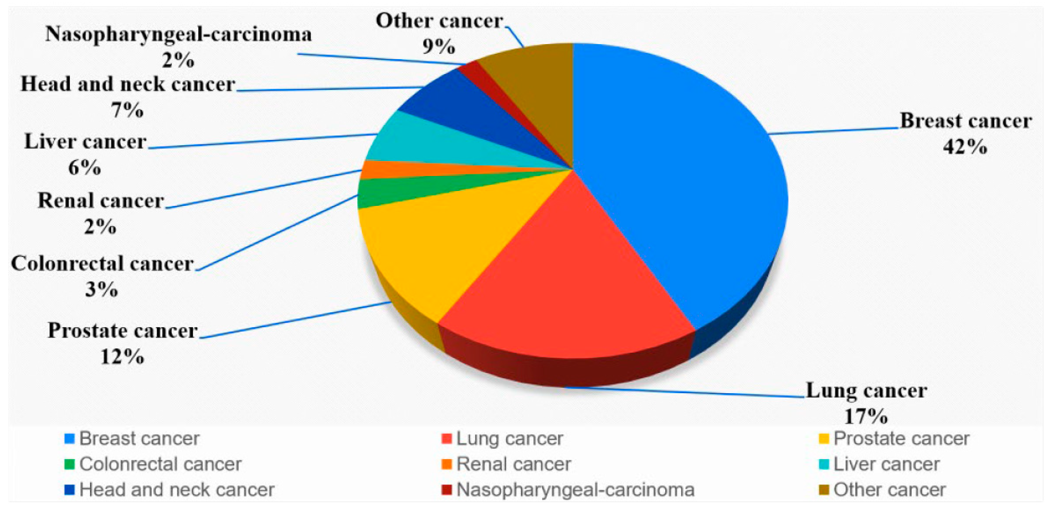
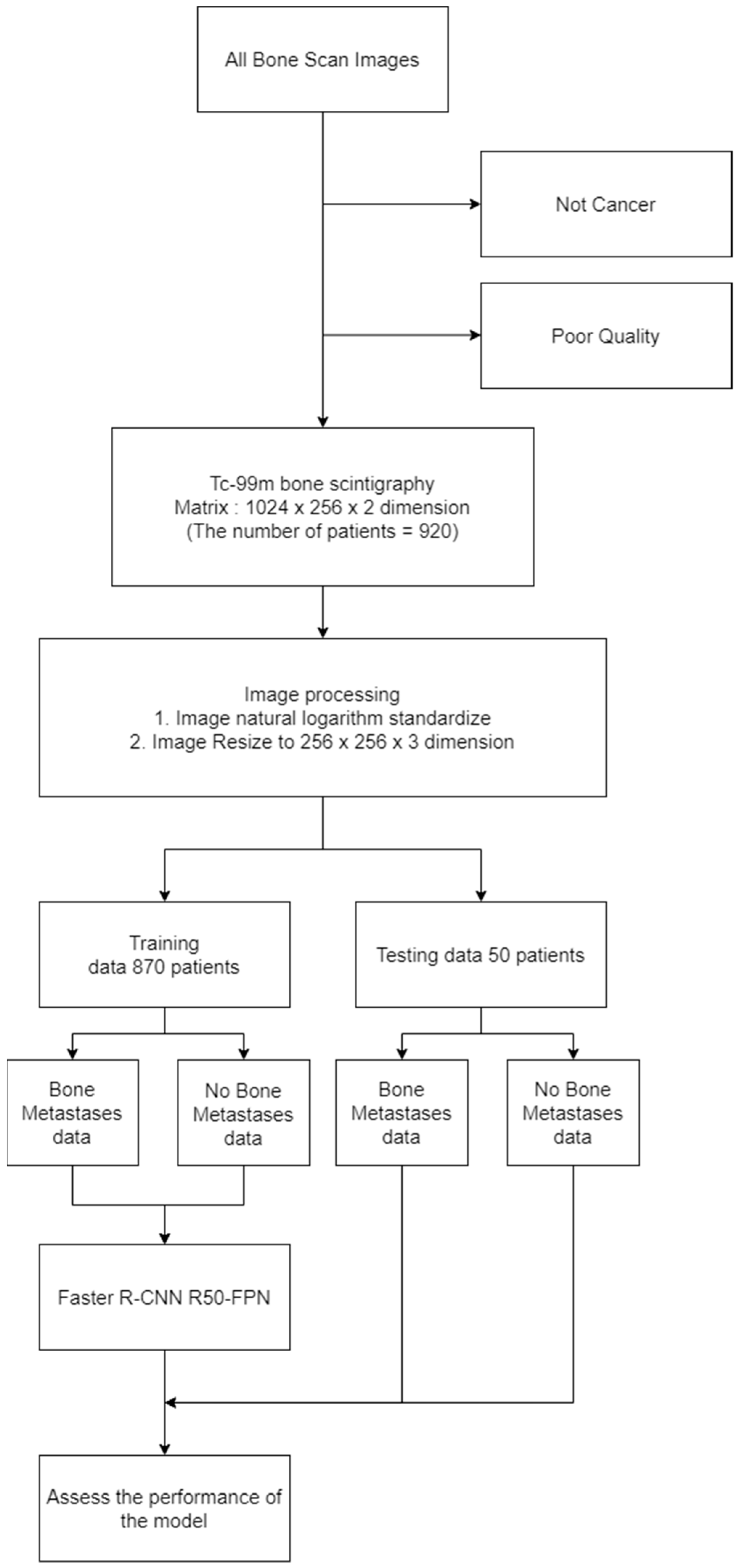
2.2. Experimental Data
2.3. Experimental Design
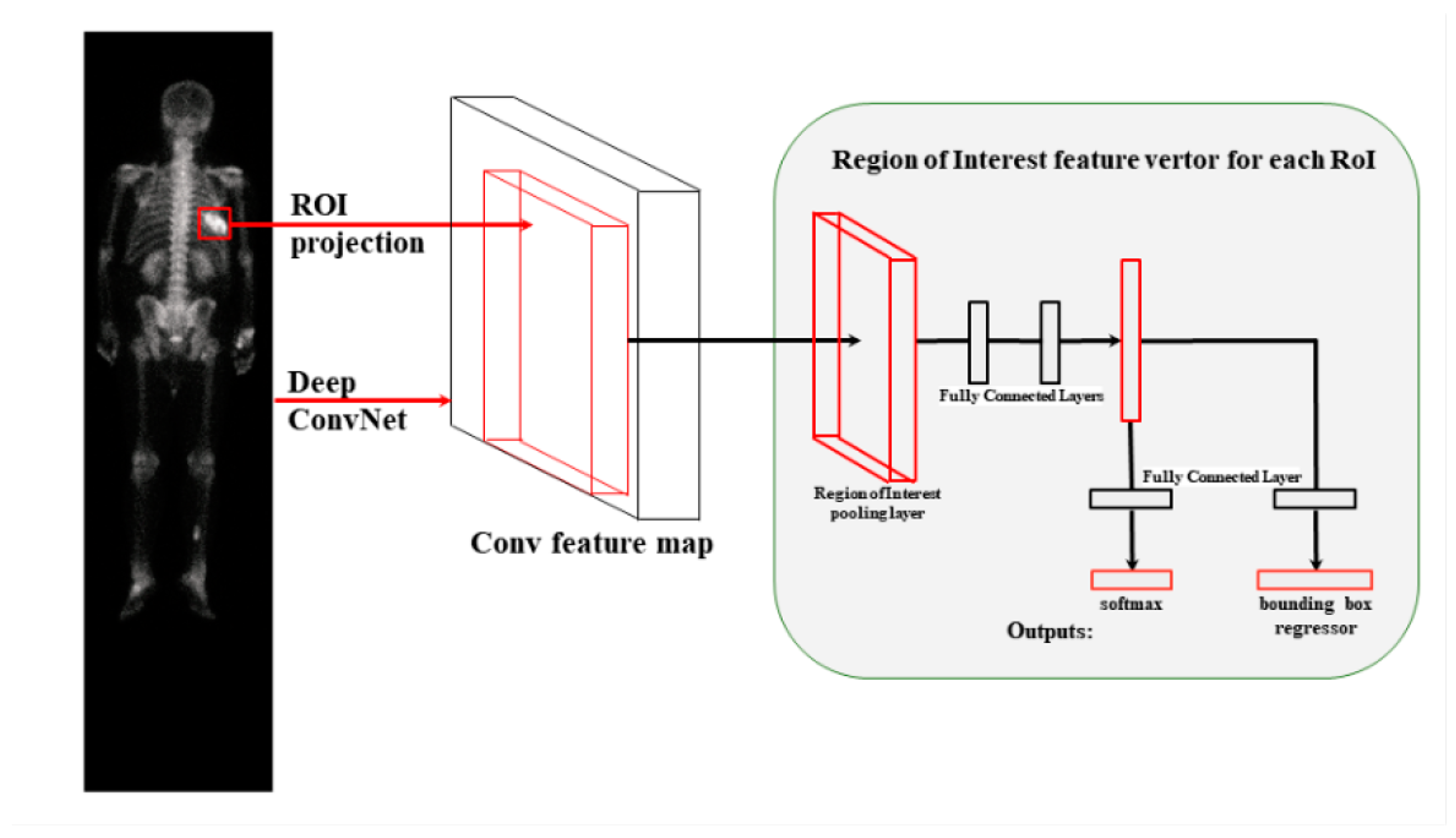
2.4. Faster R-CNN
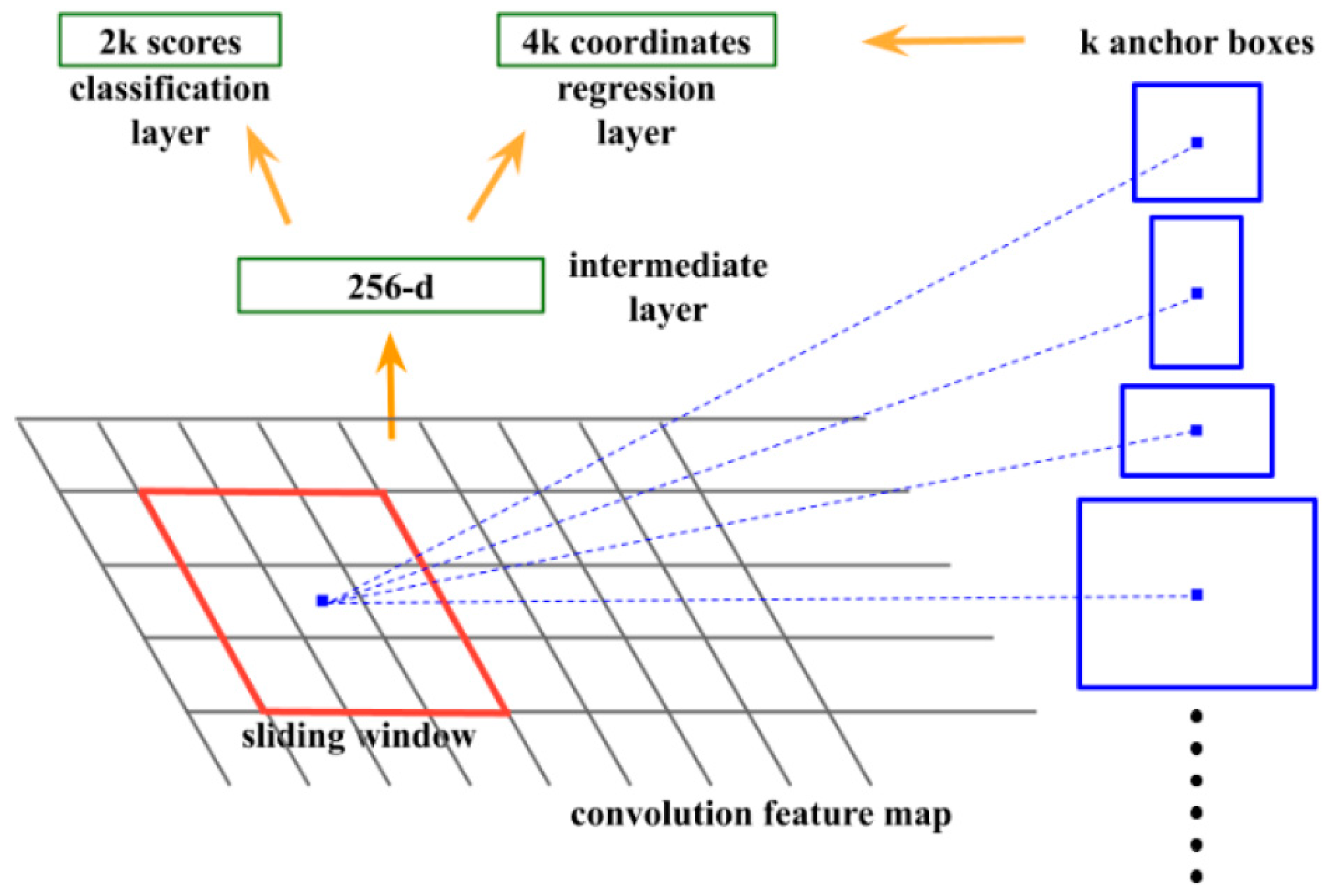
2.5. RPN
2.6. Faster R-CNN ResNet50
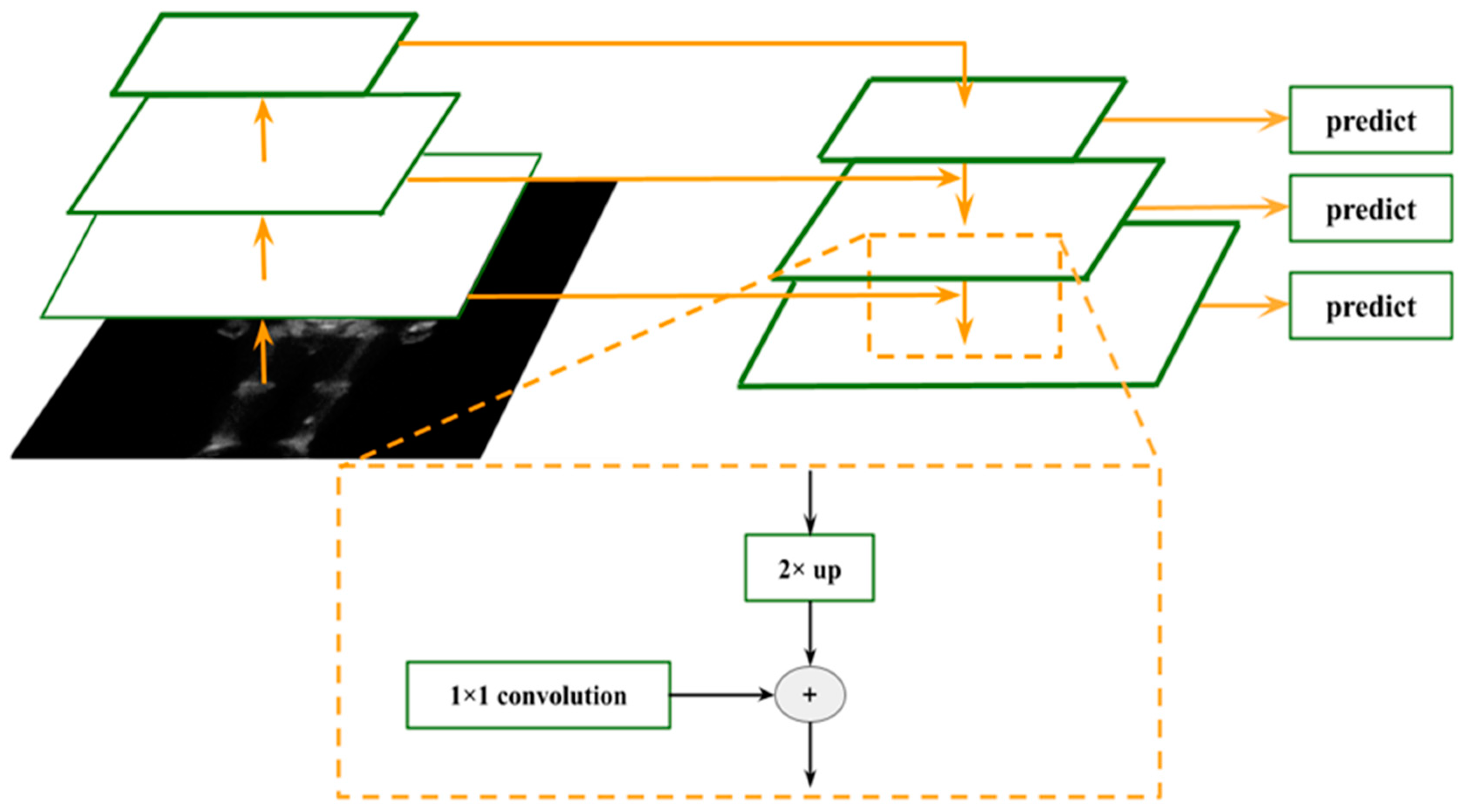
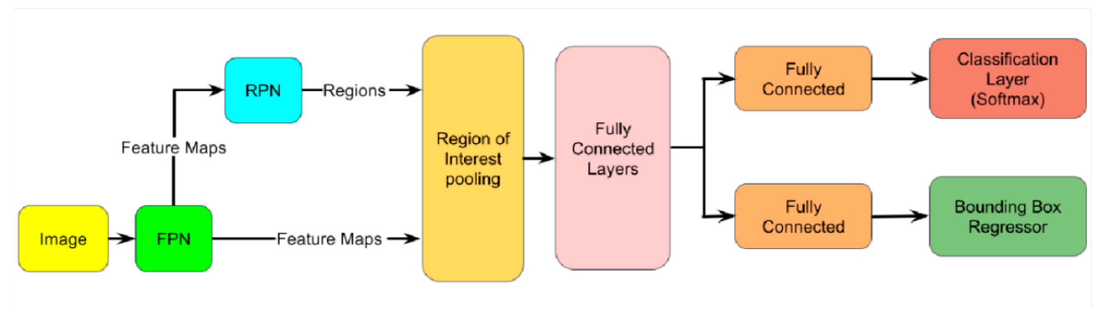
2.7. Faster R-CNN R50-FPN
2.8. Swin Transformer and YOLOR
2.9. Model Estimation
3. Results
3.1. Results of Object Detection Model and Doctor
3.2. Results of Different Doctors
3.3. Results of Different Object Detection Models
4. Discussion
5. Conclusions
Author Contributions
Funding
Institutional Review Board Statement
Informed Consent Statement
Data Availability Statement
Acknowledgments
Conflicts of Interest
References
- Brenner, A.I.; Koshy, J.; Morey, J.; Lin, C.; DiPoce, J. The bone scan. Semin. Nucl. Med. 2012, 42, 11–26. [Google Scholar] [CrossRef] [PubMed]
- Fogelman, I.; Coleman, R. The bone scan and breast cancer. Nuclear medicine annual. vp; Worldcat; Raven Press: New York, NY, USA, 1988; pp. 1–38. ISBN 0-88167-433-8. [Google Scholar]
- Shibata, H.; Kato, S.; Sekine, I.; Abe, K.; Araki, N.; Iguchi, H.; Izumi, T.; Inaba, Y.; Osaka, I.; Kato, S.; et al. Diagnosis and treatment of bone metastasis: Comprehensive guideline of the Japanese Society of Medical Oncology, Japanese Orthopedic Association, Japanese Urological Association, and Japanese Society for Radiation Oncology. ESMO Open 2016, 1, e000037. [Google Scholar] [CrossRef] [PubMed]
- Hamaoka, T.; Madewell, J.E.; Podoloff, D.A.; Hortobagyi, G.N.; Ueno, N.T. Bone imaging in metastatic breast cancer. J. Clin. Oncol. 2004, 22, 2942–2953. [Google Scholar] [CrossRef] [PubMed]
- Cook, G.J.R.; Molecular, G.V. Imaging of Bone Metastases and Their Response to Therapy. J. Nucl. Med. 2020, 61, 799–806. [Google Scholar] [CrossRef] [PubMed]
- Yuan, G.; Liu, G.; Wu, X.; Jiang, R. An Improved YOLOv5 for Skull Fracture Detection. International Symposium on Intelligence Computation and Applications. In Exploration of Novel Intelligent Optimization Algorithms. Proceedings of the 12th International Symposium, ISICA 2021, Guangzhou, China, 20–21 November 2021; Springer: Berlin/Heidelberg, Germany, 2022; pp. 175–188. [Google Scholar]
- Rani, S.; Singh, B.K.; Koundal, D.; Athavale, V.A. Localization of stroke lesion in MRI images using object detection techniques: A comprehensive review. Neurosci. Inform. 2022, 2, 100070. [Google Scholar] [CrossRef]
- Liu, B.; Luo, J.; Huang, H. Toward automatic quantification of knee osteoarthritis severity using improved Faster R-CNN. Int. J. Comput. Assist. Radiol. Surg. 2020, 15, 457–466. [Google Scholar] [CrossRef] [PubMed]
- Redmon, J.; Divvala, S.; Girshick, R.; Farhadi, A. You Only Look Once: Unified, Real-Time Object Detection. arXiv 2015, arXiv:1506.02640. [Google Scholar] [CrossRef]
- Ren, S.; He, K.; Girshick, R.; Sun, J. Faster R-CNN: Towards Real-Time Object Detection with Region Proposal Networks. arXiv 2015, arXiv:1506.01497. [Google Scholar] [CrossRef] [PubMed]
- Liu, Z.; Lin, Y.; Cao, Y.; Hu, H.; Wei, Y.; Zhang, Z.; Lin, S.; Guo, B. Swin Transformer: Hierarchical Vision Transformer Using Shifted Windows. In Proceedings of the 2021 IEEE/CVF International Conference on Computer Vision (ICCV), Montreal, QC, Canada, 10–17 October 2021; pp. 9992–10002. [Google Scholar] [CrossRef]
- Wang, C.Y.; Yeh, I.H.; Liao, H.Y.M. You Only Learn One Representation: Unified Network for Multiple Tasks. arXiv 2021, arXiv:2105.04206. [Google Scholar] [CrossRef]
- Wu, Y.; Kirillov, A.; Massa, F. Detectron2. 2019. Available online: https://github.com/facebookresearch/detectron2 (accessed on 30 January 2023).
- Girshick, R. Fast R-CNN. arXiv 2015, arXiv:1504.08083. [Google Scholar] [CrossRef]
- Sadik, M.; Hamadeh, I.; Nordblom, P.; Suurkula, M.; Höglund, P.; Ohlsson, M.; Edenbrandt, L. Computer-assisted interpretation of planar whole-body bone scans. J. Nucl. Med. 2008, 49, 1958–1965. [Google Scholar] [CrossRef] [PubMed]
- Hsieh, T.C.; Liao, C.W.; Lai, Y.C.; Law, K.M.; Chan, P.K.; Kao, C.H. Detection of Bone Metastases on Bone Scans through Image Classification with Contrastive Learning. J. Pers. Med. 2021, 11, 1248. [Google Scholar] [CrossRef] [PubMed]
- Liu, S.; Feng, M.; Qiao, T.; Cai, H.; Xu, K.; Yu, X.; Jiang, W.; Lv, Z.; Wang, Y.; Li, D. Deep Learning for the Automatic Diagnosis and Analysis of Bone Metastasis on Bone Scintigrams. Cancer Manag. Res. 2022, 14, 51–65. [Google Scholar] [CrossRef] [PubMed]
- Zhang, J.; Huang, M.; Deng, T.; Cao, Y.; Lin, Q. Bone metastasis segmentation based on Improved U-NET algorithm. In Proceedings of the 2021 4th International Conference on Advanced Algorithms and Control Engineering (ICAACE 2021), Sanya, China, 29–31 January 2021; Conference Series. Volume 1848. [Google Scholar]
- Cheng, D.C.; Hsieh, T.C.; Yen, K.Y.; Kao, C.H. Lesion-Based Bone Metastasis Detection in Chest Bone Scintigraphy Images of Prostate Cancer Patients Using Pre-Train, Negative Mining, and Deep Learning. Diagnostics 2021, 11, 518. [Google Scholar] [CrossRef] [PubMed]


| Doctor | Threshold | DSC | Doctor | Threshold | DSC | Doctor | Threshold | DSC |
|---|---|---|---|---|---|---|---|---|
| doctor A | 0 | 0.0861 | doctor B | 0 | 0.0771 | doctor C | 0 | 0.1532 |
| doctor A | 0.1 | 0.3009 | doctor B | 0.1 | 0.2970 | doctor C | 0.1 | 0.3601 |
| doctor A | 0.2 | 0.4303 | doctor B | 0.2 | 0.4337 | doctor C | 0.2 | 0.4519 |
| doctor A | 0.3 | 0.5174 | doctor B | 0.3 | 0.5299 | doctor C | 0.3 | 0.5318 |
| doctor A | 0.4 | 0.5819 | doctor B | 0.4 | 0.5915 | doctor C | 0.4 | 0.5885 |
| doctor A | 0.5 | 0.5784 | doctor B | 0.5 | 0.5924 | doctor C | 0.5 | 0.5707 |
| doctor A | 0.6 | 0.6021 | doctor B | 0.6 | 0.6098 | doctor C | 0.6 | 0.5711 |
| doctor A | 0.7 | 0.6640 | doctor B | 0.7 | 0.6210 | doctor C | 0.7 | 0.5750 |
| doctor A | 0.8 | 0.6445 | doctor B | 0.8 | 0.6103 | doctor C | 0.8 | 0.5515 |
| doctor A | 0.9 | 0.5890 | doctor B | 0.9 | 0.5342 | doctor C | 0.9 | 0.4656 |
| doctor A | 1 | 0.4800 | doctor B | 1 | 0.4600 | doctor C | 1 | 0.3800 |
| Doctor Be Prediction | Doctor Be Ground Truth | DSC |
|---|---|---|
| doctor A | doctor B | 0.7040 |
| doctor B | doctor C | 0.6545 |
| doctor C | doctor A | 0.6822 |
| Faster R-CNN R50-FPN | Faster-RCNN X101-32x8d-FPN | Faster R-CNN Swin-T FPN | YOLOR | |
|---|---|---|---|---|
| doctor A | 0.6640 | 0.5327 | 0.38 | 0.3827 |
| doctor B | 0.6210 | 0.6072 | 0.48 | 0.4832 |
| doctor C | 0.5750 | 0.5892 | 0.46 | 0.4622 |
Disclaimer/Publisher’s Note: The statements, opinions and data contained in all publications are solely those of the individual author(s) and contributor(s) and not of MDPI and/or the editor(s). MDPI and/or the editor(s) disclaim responsibility for any injury to people or property resulting from any ideas, methods, instructions or products referred to in the content. |
© 2023 by the authors. Licensee MDPI, Basel, Switzerland. This article is an open access article distributed under the terms and conditions of the Creative Commons Attribution (CC BY) license (https://creativecommons.org/licenses/by/4.0/).
Share and Cite
Liao, C.-W.; Hsieh, T.-C.; Lai, Y.-C.; Hsu, Y.-J.; Hsu, Z.-K.; Chan, P.-K.; Kao, C.-H. Artificial Intelligence of Object Detection in Skeletal Scintigraphy for Automatic Detection and Annotation of Bone Metastases. Diagnostics 2023, 13, 685. https://0-doi-org.brum.beds.ac.uk/10.3390/diagnostics13040685
Liao C-W, Hsieh T-C, Lai Y-C, Hsu Y-J, Hsu Z-K, Chan P-K, Kao C-H. Artificial Intelligence of Object Detection in Skeletal Scintigraphy for Automatic Detection and Annotation of Bone Metastases. Diagnostics. 2023; 13(4):685. https://0-doi-org.brum.beds.ac.uk/10.3390/diagnostics13040685
Chicago/Turabian StyleLiao, Chiung-Wei, Te-Chun Hsieh, Yung-Chi Lai, Yu-Ju Hsu, Zong-Kai Hsu, Pak-Ki Chan, and Chia-Hung Kao. 2023. "Artificial Intelligence of Object Detection in Skeletal Scintigraphy for Automatic Detection and Annotation of Bone Metastases" Diagnostics 13, no. 4: 685. https://0-doi-org.brum.beds.ac.uk/10.3390/diagnostics13040685